Experimental investigation of wind effect on solar panels

Scholarship@Western

Scholarship@Western

Electronic Thesis and Dissertation Repository

4-15-2013 12:00 AM

Experimental investigation of wind effect on solar panels

Experimental investigation of wind effect on solar panels

Ayodeji Abiola-Ogedengbe The University of Western Ontario

Supervisor Kamran Siddiqui

The University of Western Ontario

Graduate Program in Mechanical and Materials Engineering

A thesis submitted in partial fulfillment of the requirements for the degree in Master of Engineering Science

© Ayodeji Abiola-Ogedengbe 2013

Follow this and additional works at: https://ir.lib.uwo.ca/etd

Part of the Aerodynamics and Fluid Mechanics Commons, Civil Engineering Commons, Energy Systems Commons, and the Other Mechanical Engineering Commons

Recommended Citation Recommended Citation

Abiola-Ogedengbe, Ayodeji, "Experimental investigation of wind effect on solar panels" (2013). Electronic Thesis and Dissertation Repository. 1177.

https://ir.lib.uwo.ca/etd/1177

This Dissertation/Thesis is brought to you for free and open access by Scholarship@Western. It has been accepted for inclusion in Electronic Thesis and Dissertation Repository by an authorized administrator of

EXPERIMENTAL INVESTIGATION OF WIND EFFECT ON SOLAR PANELS

(Thesis format: Integrated Article)

by

Ayodeji Abiola-Ogedengbe

Graduate Program in Engineering Science

Department of Mechanical and Materials Engineering

A thesis submitted in partial fulfillment

of the requirements for the degree of

Master in Engineering Science

The School of Graduate and Postdoctoral Studies

The University of Western Ontario

London, Ontario, Canada

ii

Abstract

Photovoltaic Solar Panels for electricity generation are outdoor low-rise structures that are vulnerable to damage by the wind. The existing building codes do not contain information about the impact of the wind on these structures and hence do not provide comprehensive guidelines to mitigate such impact. The present study is a contribution to the ongoing efforts to codify the wind loading on solar panels. In this study, experimental investigations were conducted on the scaled model of a ground-mounted solar panel structure whose surface is geometrically similar to an inclined flat plate and mounted on three-legged support. The panel comprises of gaps, which divide it into an array of 24 smaller units. The objective of this study is to determine the wind pressure distribution on the panel and characterize the flow dynamics around it. The pressure measurements were conducted through taps connected to pressure transducers for both head-on (0o, 180o) and oblique (30o, 150o) wind directions with the panel inclined at 25o and 40o. The results indicate that larger inclination angles increased the wind forcing on the panel. At a panel inclination of 25o, velocity fields of the wind approaching head-on at 0o were captured to examine the flow field using particle image velocimetry (PIV) technique. The mean and turbulent

velocities around the panel are computed and presented. The results indicate that the gaps between each unit of the panel influenced the wind loading pattern on the solar panel.

Keywords

iii

Co-Authorship Statement

iv

Acknowledgments

I give thanks to God, who enabled me to complete this thesis.

I am grateful for the financial support of my supervisors; Dr. Kamran Siddiqui and Dr. Horia Hangan. Dr. Siddiqui dedicated countless hours to edit my drafts and provided valuable feedbacks. During the course of my research work, I am fortunate to have met Dr. Girma Bitsuamlak and Dr. Aly Sayed whose timely contributions ensured that I did not give up on this work when I could. I am grateful to Ahmed Elatar; a friend whose support I have always counted on since the beginning of my studies and through my experiments.

I am grateful to my mom, grandma and siblings, thousands of miles away for their enduring love and supports. To those I call friends here in London; your supports have been immeasurable – my housemates, friends in church and school. Thank you. Special thanks to Jennifer Ehiwario for the support and encouragements through the challenges and the success of this work.

Also, I will acknowledge friends at the Teaching Support Center – Nanda Dimitrov and Nadine Le Gros for their trainings and personal advice which helped me to navigate the challenges of graduate life in Western.

v

Table of Contents

Abstract ... ii

Keywords ... ii

Co-Authorship Statement... iii

Acknowledgments... iv

Table of Contents ... v

List of Tables ... viii

List of Figures ... ix

List of Appendices ... xii

Nomenclature ... xiii

Chapter 1 ... 1

1 General Introduction ... 1

1.1 Background ... 1

1.2 Motivation ... 5

1.3 Objectives ... 6

1.4 Thesis Layout ... 7

1.5 References ... 7

Chapter 2 ... 10

2 Experimental investigations of wind effect on a standalone photovoltaic structure .... 10

2.1 Introduction ... 10

2.1.1 Background ... 10

2.1.2 Literature review ... 11

2.2 Experimental Details ... 15

vi

2.2.2 Flow development ... 17

2.2.3 The pressure tests ... 18

2.3 Results and Discussions ... 19

2.3.1 Validation of pressure results ... 21

2.3.2 Head on, forward wind direction (0o) ... 21

2.3.3 Head on, reverse wind direction (180o) ... 24

2.3.4 Effect of the inclination angles at head on wind direction ... 26

2.3.5 Oblique wind directions (30o and 150o) ... 26

2.3.6 Drag and lift forces ... 29

2.4 Conclusions ... 30

2.5 Acknowledgement ... 31

2.6 References ... 31

Chapter 3 ... 34

3 Experimental investigations of wind effect on a standalone photovoltaic table: particle image velocimetry measurements. ... 34

3.1 Introduction ... 34

3.2 Experimental Details ... 38

3.2.1 Experimental setup and facilities ... 38

3.2.2 Description of the wind profile ... 40

3.2.3 Experimental procedure ... 42

3.3 Results ... 44

3.3.1 Mean velocities ... 44

3.3.2 Turbulent velocities ... 52

3.4 Discussions ... 57

3.4.1 Mean and turbulent velocities ... 57

vii

3.5 Conclusions ... 62

3.6 Acknowledgements ... 63

3.7 References ... 63

Chapter 4 ... 67

4 General conclusions ... 67

4.1 Summary and Discussion of Results... 67

4.2 Contributions to knowledge ... 69

4.3 Future Recommendations ... 69

4.4 References ... 70

Appendices ... 71

viii

List of Tables

ix

List of Figures

Figure 1-1: Vertical profile of wind approaching a solar panel. ... 3 Figure 1-2: Solar panel damaged by strong wind in Taiwan [5] ... 3 Figure 2-1: Image of the 1/10 scaled model of the PV structure built with aluminum (a) front view (b) back view... 15 Figure 2-2: Tap Layout on the model of the PV structure. There are 64 taps on each surface of the model shown by the open circles. ... 16 Figure 2-3: Experimental setup of the pressure test in the wind tunnel... 17 Figure 2-4: Mean wind velocity profile measured in the wind tunnel compared with the NBCC open terrain velocity profile. ... 18 Figure 2-5: Illustrations show (a) the inclined solar panel and the approaching wind, (b) the various angles and directions of the wind relative to the model during the test. ... 20 Figure 2-6: Illustration of normal, lift and drag force coefficients. ... 20 Figure 2-7: Validation of pressure test by results by comparing the Cp on the model at

30o inclination with the results of Fage and Johanssen [1] on a 29.85o inclined flat plate ... 21 Figure 2-8: Contour map of Cp+ across the PV structure shows centre similarity at 0owind

x

Figure 2-12: Comparison of Cp across the solar panel with and without the inter-panel gaps for 25o (left) and 40o (right) panel inclination. The wind approaches the model head on, at 180o. ... 25 Figure 2-13: A comparison of the Cp on the model inclined at 25o (left) and 40o (right) for two different exposures. Wind approaches the model head on, at 180o. ... 25 Figure 2-14:Plots show the effect of inclination angle when the wind approaches head on at 0o (left) and 180o (right). The Cp was generally higher on the panel at 40o than 25o at both head on wind angles. ... 26 Figure 2-15: Contour plot of pressure distribution (Cp+) over the panel inclined at 25 degree when

the wind approaches at 30o. ... 27 Figure 2-16: Cp plots across the left and right halves of the model with the wind flowing from 30o angular directions and the model inclined at 25o. The pressure distributions are not similar on both sides at this wind direction. ... 27 Figure 2-17: Cp plots across the left and right halves of the model with the wind flowing from 30o angular directions and the model inclined at 40o. The pressure distributions are not symmetrical for both sides at this wind direction. ... 28 Figure 2-18:Cpplots across the left and right halves of the model with the wind flowing from 150o angular directions and the model inclined at 25o. The pressure distributions are not similar on both sides at this wind direction... 29 Figure 2-19: Copilots across the left and right halves of the model with the wind flowing from 150o angular directions and the model inclined at 40o. The pressure distributions are not similar on both sides at this wind direction... 29 Figure 2-20: The drag coefficients CD and lift coefficients CL on the panel due to wind impacting

xi

Figure 3-3: The vertical profile of the mean wind velocity ... 41 Figure 3-4: Illustration of the four Measurement Planes showing the shadowed region and the vertical profile of the approach wind. ... 43 Figure 3-5: Vector Plot of the Mean Velocities at each grid point for the four measurement planes labeled (a) Section I (b) Section II (c) mean vertical velocity Section II (d) mean streamwise velocity at section II, (e) section III (f) mean vertical velocity Section III (g) mean streamwise velocity at section III, and (h) Section IV at ReL = 4 x 106. ... 48

Figure 3-6: Profile of the mean velocity at various spatial locations in all measurement sections across the photovoltaic panel for ReL = 4 x 106 (o) and ReL = 1 x107 (*). ... 51

Figure 3-7: Vector Plot of the Turbulent velocities at each grid point for the four measurement planes labeled (a) Section I (b) Section II (c) Section III and (d) Section IV at ReL = 4 x 106. ... 54

Figure 3-8: Profiles of the stream-wise RMS turbulence intensity at various spatial locations in all measurement sections across the photovoltaic panel for ReL = 4 x 106 (o) and ReL = 1 x107 (*). . 56

Figure 3-9: Profile of the cross-stream RMS turbulence intensity at the four spatial locations in all measurement sections across the photovoltaic panel for ReL = 4 x 106 (o) and ReL = 1 x107 (*). . 58

xii

List of Appendices

xiii

Nomenclature

A Area (m2)

B Panel breadth (m)

C width of upstream structure (m) CD Coefficient of drag

CL Coefficient of lift

CN Normal force coefficient

Cpi Coefficient of pressure at tap, i

Cp+ Pressure coefficient at upper surface of panel Cp- Pressure coefficient at lower surface of panel

∆ Differential pressure coefficient of taps on opposite surfaces

∆ Differential pressure coefficient at tap, i

D Drag (N)

H Height (m)

h+ hole

L Length (m)

LF Lift (N)

Pi Pressure at tap, i

Pref Reference pressure

xiv ReL Reynolds number (length based)

S Distance between structures (m) u velocity (m/s)

ug gradient wind velocity or speed (m/s)

uref reference velocity (m/s)

W Width (m)

x/L normalized position on panel length y/W normalized position on panel width z height from the ground (m)

zg gradient height (m)

Ground surface roughness (m)

zref reference height (m)

Greek Symbols

1 ∝⁄ Terrain exponent ∝ Inclination angle (o)

Latitude of site (o) Density (kg/m3)

Abbreviations

xv BLWTL Boundary Layer Wind Tunnel Laboratory CdTe Cadmium Telluride

CFD Computational Fluid Dynamics

CMOS Complementary metal-oxide-semiconductor DAQ Data Acquisition

FiT Feed-in-tariff LE Leading edge NaN Not-a-number

NBCC National Building Code of Canada PIV Particle Image Velocimetry PV Photovoltaic

Chapter 1

1

General Introduction

1.1 Background

The global electricity generation is projected to be almost double from 18.8 trillion kWh in 2007 to 35.2 trillion kWh in 2035 [1] to meet the electricity demand caused by two major factors; population growth and the improved lifestyle particularly in the developing countries. Fossil fuels, in particular coal and natural gas have been projected as the dominant energy source contributing almost 70% of the energy supply for the power generation to meet this growing demand [1]. This heavy reliance on fossil fuel in particular on coal to meet the growing energy demand, will have severe consequences on the global climate which could jeopardize the living environment of the future generations. Due to the harmful effects of fossil fuels on the environment, there is a growing concern on limiting their use and switching to clean alternative energies such as solar, wind and biomass, to meet the energy needs and reduce the consumption of fossil fuels and their carbon footprint. One of the widely commercialized solar energy technologies is the photovoltaic (PV) solar cells that convert the sunlight directly into electricity. The solar cells are made of

semiconductors materials such as Silicon or Cadmium Telluride (CdTe). Sunlight contains energy particles called photons. When light from the sun incidents on a solar cell, the photons are absorbed by the semiconductor material. The absorbed photons knock electrons (e-) out of their atoms in the semiconductor creating a hole (h+). The design of the

semiconductor diode ensures that the released electrons move in a single direction and produces electricity [2]. Sets of solar cells are combined to make a solar panel. They are installed by fastening them to a framework or support structure as standalone units or as an array of PV units. A standalone solar PV structure may also comprise of several individual panels arrayed as a single structure.

to homeowners, farmers and businesses to generate electricity from solar panels and sell it to the electricity grid at a much higher rate than the rate at which they buy electricity from the hydro utility. For example, for less than 10 kW setups, the government pays 54.9cents and 44.5cents per kilowatt-hour for rooftop solar panels and ground-mounted solar panels respectively [3]. Last year, the private sector in Ontario reportedly spent over C$9 billion in renewable energy projects [4]. This is an indication of the economic importance of solar panel investments. One of the main obstacles in the wide spread commercialization of PV solar panels is its cost, which resulted in a long payback period. The risk factor associated with its partial or complete damage by wind further elevates the financial risk of the customer and hence, its marketing and commercialization. Currently, the impact of wind loading on the PV panels (stand alone or array format) is not well understood and hence, the associated damage risk is not well quantified. Furthermore, this lack of information also hinders the aerodynamic design improvement of the solar panels to mitigate this risk. Solar panels are commonly installed with an inclination angle equal to the latitude of the site. Studies have shown that as wind impinges on an inclined solar panel, it flows around it and induces unequal pressure on its two surfaces. The surfaces of the solar panels thereby experience the drag force in the direction of the wind flow and lift force in the direction perpendicular to the flow. These forces produce the torque. The drag force is expressed as, = 1 2 , while the lift force is given as, = 1 2 ,

where, , , refers to air density, wind velocity, projected area, coefficients of lift and drag, respectively. Torque is expressed as the product of force and the displacement vector from the point where the force is applied. These forces are depicted schematically in Figure 1-1. In case of strong winds these forces and the resulting torque could damage the solar panel structure. An example of such damage is shown in Figure 1-2 where a severe typhoon damaged the solar collectors in Taiwan [5]. Although there are practical limits to the protection of solar panels in extreme wind situations, nonetheless proper understanding of the wind phenomenon at the site can help prevent solar panel damages by more frequent wind gusts.

one of the early projects that defined wind engineering studies [6, 7]. Wind codes have been developed as receptacles for the knowledge obtained from wind engineering. Investigations of wind effect on low-rise structures are now common [8-10] and they have provided valuable data into various wind codes. However, existing wind codes do not yet have a guide for solar panels. The National Building Code of Canada states that structures should be designed so that they can withstand pressures and suction from the strongest wind generated in that area based on wind statistics.

Figure 1-1: Vertical profile of wind approaching a solar panel.

Figure 1-2: Solar panel damaged by strong wind in Taiwan [5]

Engineers can determine the wind loading using any of the three methods proposed by the

enclosed structures. Eligible structures for the analytical method should not be on a site for which wake buffeting will be considered [12]. Solar Panels do not meet the requirements for both the simplified and analytical methods. This is because solar panels are known to be susceptible to vortex shedding and wake buffeting [13, 14]. Therefore, studies of wind effect on solar panels are conducted using wind tunnel method or Computational Fluid Dynamics (CFD). However, the accuracy of CFD modeling relies on its validation with the

experimental data. The common techniques used in wind tunnel studies of structures are flow visualizations, hot-wire anemometry, local pressure taps and high frequency force balance [15].

Full scale test of the solar panel in the wind tunnel is not practical due to the blockage restrictions. Wind tunnel testing guidelines set by ASCE [11] requires that the projected area of the model should be less than 8% of the wind tunnel cross sectional area to avoid

blockage effects. Similitude between model and full-scale prototype must also be satisfied. Some notable wind tunnel studies on solar panels are available in the open literature. The report of Miller and Zimmerman [17] on their study commissioned by the United States Department of Energy indicates that fences and barriers can be used to reduce the wind load on solar arrays and end plates are suitable to reduce large loads on individual panels. The researchers arrived at this conclusion after observing that structures upstream of the flow shelter those located downstream. The sheltering effect on downstream panels was also observed by Radu et al. [18] from the wind tunnel studies of solar panel models installed on the roof of a scaled model of a five-storey building. Using CFD studies, Shademan [13] estimated that for a solar panel inclined at 30o, beyond a critical spacing of ⁄ = 1 (where S is the distance between both structures and C is the width of the upstream structure), the sheltering effect of an upstream structure on the wind load of the downstream panel becomes negligible.

Kopp et al. [14] tested an array of six slender solar modules in the wind tunnel to determine the location of the highest system torque and the critical loading angle of the wind

based on the pressure coefficient, ∆. They recommended ∆ value of -0.3 for the upward

acting force and 0.2 for the downward acting force on a single solar panel on the rooftop. The uplift force on the model of a solar panel fitted with water heaters in Taiwan was measured in the wind tunnel by Chung et al. [5]. They recommended fitting a guide plate on the solar panel to reduce the wind uplift.

Past studies also examined the impact of specific geometrical features on the wind loading of solar panels. Radu and Axinte [20] studied the wind load on the structural supports of solar panels and the load transmitted to building attics on which the solar panels were installed. Wu et al [21] tested the model of a heliostat, which has similar geometry as a solar panel. They examined the effect of the gap of various sizes on the facet of the heliostat. They determined that while the gaps do increase the wind loading on the structure, they need not be considered for structural designs of the system, as they constitute very small fraction of the total area.

Various wind studies measured the wind load on specific geometrical shape of solar modules. Each test and its conclusions were therefore unique to the configuration of the solar structure tested [13-20]. Few studies investigated the dynamics of the wind flow around the solar panels [13, 14 and 18].

1.2 Motivation

are past studies, which estimated the wind loads on these structures, but the results of those studies cannot be applied in a generic sense since they are based on specific geometries. Also, the mechanisms by which the wind interacts with the solar structures remain an under-explored research area. The present work is a contribution to the on-going efforts in

establishing a standard knowledge base of the wind loading and their effect on typical solar panels.

1.3 Objectives

The objectives of this research are:

1. To study and measure the load exerted by the wind on a solar panel structure with regards to its geometrical configurations and the wind environment into which it is situated.

2. To investigate and understand the mechanisms by which the wind impacts and affects a panel structure.

This research provides a framework to investigate wind effect on PV panels and also provide benchmark data that could be used by the industry, for building code improvement as well as for the CFD modeling.

The design of the PV solar panel used in this study was based on the panels produced by First Solar (the industrial partner on this project). The standalone model has been

similarity is no longer necessary. This satisfies another requirement for the minimization of Reynolds number effect on pressure and forces for the wind tunnel tests [10].

Table 1-1: Percentage Blockage of the BLWT 1 and BLWT 2 by the solar panel model

Tunnel Smallest Cross Section (m2) Blockage (%)

BLWT 1 3.6 3.4

High Speed Test Section BLWT 2 8.5 1.44

Low Speed Test Section BLWT 2 20 0.61

1.4 Thesis Layout

The first chapter is an introduction to the research work, which provides a description of the problem that this work aims to address, and the justification for it. A brief historical

narrative of wind engineering and the methodologies it employs are given followed by a short review of past literatures on the subject of the research. The motivation and the objectives of this work are then presented. Chapter two is a report of the pressure measurement conducted on the scaled model of a solar panel. The chapter presents the quantitative results of the pressure force exerted on the solar panel by the wind. The third chapter presents the experimental investigation into wind flow across the solar panel. Both qualitative and quantitative descriptions of the flow are presented with the aim of

understanding the dynamics of the flow that contributes to the wind loads measured in chapter two. The fourth chapter presents a general conclusion based on the measurements reported in chapters two and three in a bid to understand how the wind flow impacts and affects the given solar panel.

1.5 References

[1] International Energy Outlook 2010, Report # DOE/EIA-0484, US Department of Energy, July 2010.

[2] Gray, J. L. (2003). The physics of the solar cell.by A. Luque, S. Hegedus.–Chichester:

[3] Ontario Power Authority. Generate Power... and Money. 2011; Available

at:microfit.powerauthority.on.ca/sites/default/files/news/FIT-mFITPriceScheduleV2.0.pdf. Last accessed 03/24, 2013.

[4] Government of Ontario. Electricity prices are changing. 2011; Available at: http://www.mei.gov.on.ca/en/pdf/EnergyPlan_EN.pdf. Last accessed 01/21, 2013. [5] Chung, K., Chang, K., & Liu, Y. (2008). Reduction of wind uplift of a solar collector model. Journal of Wind Engineering and Industrial Aerodynamics, 96(8), 1294-1306.

[6] Cochran, L. S. (2002, June). Early Days of North American Wind Engineering: An

Interview with Professor Cermak about Professor Davenport. In Proceedings of the

Engineering Symposium to Honour Alan G. Davenport for His Forty Years of

Contributions. London, Canada: University of Western Ontario.

[7] Davenport, A. G. (2002). Past, present and future of wind engineering. Journal of Wind

Engineering and Industrial Aerodynamics, 90(12), 1371-1380.

[8] Stathopoulos, T. (1984). Wind loads on low-rise buildings: a review of the state of the art. Engineering Structures, 6(2), 119-135.

[9] Uematsu, Y., &Isyumov, N. (1999). Wind pressures acting on low-rise buildings.

Journal of Wind Engineering and Industrial Aerodynamics, 82(1), 1-25.

[10] Peterka, J. A., Tan, L., Bienkiewcz, B., &Cermak, J. E. (1987). Mean and peak wind

load reduction on heliostats (No. SERI/STR-253-3212). Colorado State Univ., Fort Collins

(USA).

[11] Structural Engineering Institute. (2006). Minimum design loads for buildings and other

structures (Vol. 7, No. 5). American Society of Civil Engineers (ASCE).

[12] Hangan, H., & Vickery, B. J. (1999). Buffeting of two-dimensional bluff bodies.

[13] Shademan, M. (2010) CFD Simulation of Wind Loading on Solar Panels. (MESc Dissertation).London, Ont., School of Graduate and Postdoctoral Studies, University of Western Ontario.

[14] Kopp, G. A., Surry, D., & Chen, K. (2002). Wind loads on a solar array. Wind and Structures, an International Journal, 5(5), 393-406.

[15] Rhee, J., Nguyen, C., Grace, M., & Thu, A. (2011).An effective, low-cost mechanism for direct drag force measurement on solar concentrators. Journal of Wind Engineering and

Industrial Aerodynamics, 99(5), 665-669.

[16] Hosoya, N., Peterka, J. A., Gee, R. C., & Kearney, D. (2008).Wind Tunnel Tests of

Parabolic Trough Solar Collectors. NREL/SR-550-32282, May 2008, Golden, Colorado:

National Renewable Energy Laboratory.

[17] Miller, R., & Zimmerman, D. (1979). Wind loads on flat plate photovoltaic array fields.

Final Report Boeing Engineering and Construction Co., Seattle, WA, 1.

[18] Radu, A., Axinte, E., & Theohari, C. (1986). Steady wind pressures on solar collectors on flat-roofed buildings. Journal of Wind Engineering and Industrial Aerodynamics, 23,

249-258.

[19] Geurts, C. P. W., & Steenbergen, R. D. J. M. (2009). Full scale measurements of wind loads on stand-off photovoltaic systems. In 5th European & African Conference on Wind

Engineering (EACWE), Florence, Italy.

[20] Radu, A., &Axinte, E. (1989). Wind forces on structures supporting solar

collectors. Journal of Wind Engineering and Industrial Aerodynamics, 32(1), 93-100.

[21] Wu, Z., Gong, B., Wang, Z., Li, Z., &Zang, C. (2010). An experimental and numerical

Chapter 2

2

Experimental investigations of wind effect on a

standalone photovoltaic structure

2.1 Introduction

2.1.1

Background

Photovoltaic (PV) or solar modules are becoming increasingly popular for domestic as well as industrial electricity generation. Advancements in solar energy technology continue to improve their overall efficiency and long-term reliability. These improvements are motivated by the continual depletion of other sources of energy especially fossil fuels, which are also source of increasing environmental concerns. Among various alternative sources of energy, PV modules are the fastest growing and most popular globally with worldwide annual investments exceeding US$100 billion [1]. PV modules are vulnerable to wind damage; nevertheless there are no provisions of wind load in building standards and codes to design these structures. This is a major motivation for this study.

Wind load on structures is usually estimated experimentally in the wind tunnel or using computational fluid dynamics (CFD). When carefully and well carried out, the results from experiments can be used to validate the results obtained using CFD (for example, see Meroney [2]). To conduct a successful wind tunnel test, the structure is subjected to the same wind conditions that exist on the physical site. This involves matching the mean wind velocity profile, the turbulence intensity profiles and the ratio of the test structure’s height to ground surface roughness (Jensen number,$ ⁄ ) on the site with that in the wind tunnel. The common instrumentation for load measurements in wind tunnel experimentation

includes load cells and pressure transducers. While load cells measures the overall load on a structure, the pressure transducer instrumentation, also adopted in the present study, can be used to measure the pressure load at several points simultaneously on upper and lower surfaces of the PV panel. In this study, the net pressure coefficients across the solar panel are measured and the effects of variable parameters such as wind terrain exposure,

inclination angle and the gaps between individual panels are presented to produce the forces acting on the PV panel.

2.1.2

Literature review

The nature of the load induced on a structure by the wind depends, largely on the

characteristics of the wind such as its direction, speed, exposure conditions and the shape of the structure. Ground mounted PV modules, which are the subject of this study, are typically low-rise structures. They are therefore immersed within the lowest region of the

atmospheric boundary layer (ABL) where the flow of the wind is highly unpredictable due to the intense turbulence actions [3]. The mean velocity profile of the wind in this region is largely influenced by the ground roughness. Although in nature, for any particular terrain, roughness cannot be accurately determined owing to variations in the size, shape,

The wind loads on various types of solar modules had been measured in the wind tunnels and reported in the literature. Early examples include the wind load experimental tests on arrays of flat plate PV panels, commissioned for testing by the US Department of Energy [8]. The results of the test show that upstream flow sheltering elements such as barriers and fences can be used to reduce the wind loads on PV arrays while end plates were found most suitable in reducing the large load measured on the panels at the corners of the array. Radu et al. [9] tested an array of solar panel models, mounted on the roof of a scaled five storey-building model in a boundary layer wind tunnel. Their tests were performed on three different building models with flat roof. Each building had different kind of attics. The results showed that the front row panels had higher pressure and force coefficients. These front row panels shelter the panels behind them from the wind action. In subsequent studies, the lift forces on the support structures of these panels were also investigated [10]. They concluded that using appropriate building attics could reduce wind loads on PV modules installed on building rooftops. Wood et al. [11] also tested PV modules mounted on the flat rooftops of a scaled building model in a wind tunnel. The pressure on the scaled building roof was simultaneously measured which agreed well with the full-scale results of the Texas Tech experimental building. In the test, they varied both the clearance height between the rooftop and the panel and the lateral spacing between the panels. Except at the leading edge where slight variation was recorded, their results showed no significant changes in the overall pressure on the modules from the variation of the clearance height and panel spacing.

wind direction, corresponded with a pressure coefficient,valueof -0.55. A differential

pressure coefficient, ∆value of -0.3 for the upward and 0.2for the downward acting force was recommended for a single solar panel on such rooftops.

A 1/3 scaled model of a sun-tracking PV modules [14] were tested by Velicu et al. [15] in an open circuit wind tunnel. The drag and lift forces on the PV modules were measured using force transducers. The results showed that the force coefficients on the PV panel increased as the panel tilt angle increased from 0o to 90o.The force coefficients also increased as the wind velocity increased. Chung et al. [16] conducted wind tunnel tests to investigate the uplift on flat-plate PV collectors used for water heating. The PV modules were inclined at an angle of 25o. The pressure measurements were taken along the centerline of the panel surfaces. A guide plate was attached to the test model of the PV collector to reduce the wind uplift. The effectiveness of this guide plate was investigated by varying its angular orientation at wind velocities ranging from 20m/s to 50m/s. The results showed that the differential pressures coefficients ∆ were highest at the front, lower edge of the panels, similar to observations by Shademan [17]. The ∆ reduced downstream of the panel and steadily rise towards the rear edge. The heights of the panel from the ground were varied during the tests. The result showed that the differential pressure coefficient, ∆ close to the rear edge increased with the height, thereby reducing the wind uplift. The least wind uplift was measured when the guide plate was installed at an angle of 90o to the wind direction at the rear of the PV collector.

showed that the flow stagnated at the windward face of the concentrator while separation was observed at the leeward face.

Shademan [17] carried out wind load investigations on standalone and array PV modules using CFD. Six configurations of the standalone solar panel were tested. Their results were validated with the experimental results of a flat plate [19]. The results showed that as the inclination angle of the standalone panel increased, the drag force induced by wind load also increased. The tests were conducted at three wind angles of 30o, 60o and 90o. In all of the cases, maximum drag was produced at wind angle of 90o and on the panels at the bottom row of a standalone system. Panels at the front row of arrays shelter other panels from the wind, therefore reducing the drag force experienced by the sheltered panels. However, Shademan [17] identified the critical spacing between the panels, beyond which the drag force reduction on the downstream panels was not significant. Meroney [2] used different turbulence models to simulate the flow around PV modules. The study estimated the drag, lift and overturning moments on the solar panel support systems. Static pressure results on the panels at 0o and 180owind angles showed higher pressures at the front rows of panels, consistent with the experimental observations of Radu et al. [9] and Shademan [17]. Wu et al. [20] investigated the effect of the gaps between panels on the surface of a heliostat was investigated through CFD and experimental tests. Heliostats have similar geometrical configurations as PV panels. A 1 10⁄ scaled model of the heliostat was used for the wind tunnel experiments, similar to the length scale of this current study. The computational model of the CFD test was greatly simplified due to the huge cost of modeling the flow near the gap. Both the experimental and numerical results showed that the overall wind load slightly increased with an increase in the gap size. The CFD results showed that this increase was due to the flow acceleration through the gap, which caused a decrease in the static pressure at the gap’s outlet. Therefore the overall drag force increased due to the resultant decrease in the leeward pressure coefficient.

This present study was experimentally conducted in a boundary layer wind tunnel. The aim is measure the wind load on the PV module, and to determine the effect of varying

model and its flat plate equivalent (without the gaps between individual panels) will also be presented.

2.2 Experimental Details

2.2.1

Model and instrumentations

The model of the PV structure for this study was built at the University Machine Shop of the University of Western Ontario using aluminum. It is a one-tenth scaled replica of its

prototype and it is fitted with a weighted disc at its support to give it the required balance. The full scale prototype of this model consists of 24 individual panels in a 4 x 6 array which are held together with hinges thereby leaving gaps between each panel. The top plates of the PV structure model were machined from two flat aluminum plates and grooves were

machined to create the gaps between each of the 24 panels. Its overall dimensions are 0.72m × 0.24m × 0.17m and the support legs are spaced 0.3m apart. The model is adjustable for different inclination angles during the tests. To connect the instrumentation, a total of 128 holes or “taps” were drilled on the two aluminum plates that made up the upper and lower flat surfaces of the model. Vinyl pressure tubes of length 50.8cm and diameter0.24cm were sandwiched between the aluminum plates, with one end connected to the taps and the other end extending out from both sides of the model. This ensures that the upper and lower surfaces of the model were not obstructed with the pressure tubes. The model is shown in Figure 2-1 and the layout of the taps on the surfaces of the model is shown in Figure 2-2.

Figure 2-1: Image of the 1/10 scaled model of the PV structure built with aluminum (a) front view

Figure 2-2: Tap Layout on the model of the PV structure. There are 64 taps on each surface of the

model shown by the open circles.

The free end of each pressure tube then connects to another tube of the same length and diameter via short brass restrictors. These restrictors add the needed damping to the pressure instrumentation system. The free ends of these other tubes then connect to 8 scanners devices manufactured by Scanivalve Corporation. Each scanner connects to 16 pressure tubes from the model.

The scanner devices are transducers, which convert the pressure, read at each tap to an electrical signal and transmit it to the wind tunnel’s computerized data acquisition (DAQ) system. Each of the eight scanners is connected to eight separate channels on the wind tunnel DAQ system. A ninth channel on the wind tunnel DAQ connects to pitot-tube

devices placed near the model to measure the approach velocity and the free stream velocity at an undisturbed height above the model. The pressure data, in volts collected during the tests were analyzed and transformed to coefficient of pressure, values. The setup of the

Figure 2-3: Experimental setup of the pressure test in the wind tunnel.

2.2.2

Flow development

The study was conducted for an open terrain wind exposure scaled for testing models up to 1:20. The pressure tests were conducted at the Boundary Layer Wind Tunnel Laboratory (BLWTL 1) at the University of Western Ontario. This is an open return wind tunnel, which has a length of 33m and a width of 2.4m.Its height varies from 1.5m at the entrance to 2.15m at the test area. This wind tunnel is able to simulate wind profiles at the typical scale of ~1:400. Since the PV structure is a low-height structure, it is physically immersed within the lowest 10m of the atmospheric boundary layer (ABL). Therefore only the flow at this region was modeled in the wind tunnel. The wind profile representative of the open terrain exposure for this test was obtained after various trials. The flow conditioning elements used to model the flow include three isosceles triangular spires, rectangular roughness blocks, a fence and a bar trips. These elements were positioned upstream of the model. The ensuing wind velocity profile closely matches the mean wind velocity profile in an open terrain exposure obtained from the NBCC using the power law given as;

%& = '( ⁄ )' * ∝ ⁄

Where _' is the gradient wind speed, and1 ∝⁄ , the terrain dependent exponent is given as 0.16 in the NBCC [22]. The values of _+,- and _+,- for the terrain were determined

following the reverse method used by Shademan [18]. The comparison of the NBCC profile and the measured profile from the experiment are shown in Figure 2-4. The wind tunnel tests were repeated with the ground roughness elements removed to create a different smooth exposure. Therefore the effects of the ground roughness on the wind load across the photovoltaic panel were investigated.

Figure 2-4: Mean wind velocity profile measured in the wind tunnel compared with the NBCC open

terrain velocity profile.

2.2.3

The pressure tests

from both sides of the model. The results presented here include those for two head on angles, 0o and 180o and two oblique angles, 30o and 150o (Figure 2-5).

2.3 Results and Discussions

As previously described, a total of 128 measurement taps are situated on both surfaces of the PV model. The non-dimensional pressure coefficient values at various taps, on both surfaces of the model, %& were obtained by converting the pressure measured at each tap %1&to the

dimensionless form, using the dynamic pressure,2 at the reference height according to equation 2.2.

%& =3453₉678 2.2

Where2 = *:_+,-, and the reference height is taken at the lowest point of the inclined model’s surface. The pressure coefficient values on the model’s surface, which faces the approaching wind are considered as positive, (Cp+) while the pressure coefficients measured

on the opposite surface are negative (Cp-).Therefore, the net pressure (∆;) is the aggregate

of the pressure coefficient values on adjacent taps on the model. Such that

∆= <+ 5 2.3

The net pressures exert normal forces on the panel. The normal force coefficients ₌ on the surface, s of the panel can be obtained by integrating ∆ over the breadth, B.

> =_?*@ ∆? %s&ds 2.4

(a)

(b)

Figure 2-5: Illustrations show (a) the inclined solar panel and the approaching wind, (b) the various

angles and directions of the wind relative to the model during the test.

Figure 2-6: Illustration of normal, lift and drag force coefficients.

Lift,

2.3.1

Validation of pressure results

The experimental results of Fage and Johanssen [19] have been a suitable benchmark for studying the pressure load due to flows over inclined flat plates. To validate the results from this study, the coefficient of pressure on the PV model without the gaps and inclined at 30o was compared with the coefficient of pressure results on the flat plate experiment of Fage and Johanssen[19] at almost similar inclination angle of 29.85o. The wind flows head on, at angle 0o to the test models in both experiments. The leading edge (LE) is the lower end of the plate, while the trailing edge (TE) is the higher end. The plot of the result in Figure 2-7 shows that the Cp+ at the upper surfaces of the PV model closely matches the flat plate result. At the back of the panel however, the 5on the PV model was slightly lower than the flat plate’s. This can be attributed to the influence of the three-legged support structures, which are absent in the experimental flat plate model of Fage and Johanssen [19].

Figure 2-7: Validation of pressure test by results by comparing the Cp on the model at 30o inclination

with the results of Fage and Johanssen [1] on a 29.85o inclined flat plate

2.3.2

Head on, forward wind direction (0

)

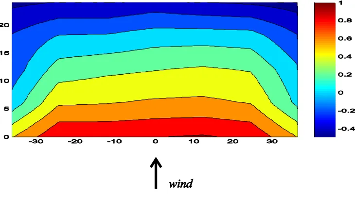
Figure 2-8: Contour map of Cp+ across the PV structure shows centre similarity at 0owind direction

The pressure distributions on either half of the panel are similar at this wind angle as can be seen from the contours. The contour plot also reveals that the magnitude of the pressure coefficients is largest at the leading edge where the flow first impinges on the model. Shademan [17] had previously identified these locations as critical loading areas on PV panels of similar geometry at 0o wind direction. The pressure induced by the wind on the surface reduces towards the trailing edge of the model.

Figure 2-9: Plots compare the effects of the gaps on the Cp across the panel for both the 25o (left)

and 40o (right) inclined panel at 0o wind direction.

Effects of terrain exposure: The test results for the open terrain exposure were compared with a smooth exposure to investigate the effect of exposure change on the pressure values. The plots in Figure 2-10 show the comparison. The pressure measured at the leading edge of the panel in open terrain exposure was used as the reference pressure to normalize pressure measurements at both exposures.

within the surface boundary layer under smooth exposure. This effect is more pronounced on the model at 40o inclination.

2.3.3

Head on, reverse wind direction (180

)

When the flow approaches the solar panel head-on in the reverse direction, i.e., 180o degree, the lower surface now faces the approaching wind while the upper surface lies in the wake of the wind flow. The pressure distribution on the lower surface, which now faces the oncoming wind, is also similar across the mid plane. The largest net positive pressures due to the wind are exerted on the leading edge of the model as seen in Figure 2-11. This edge had been the trailing edge in the 0o wind direction. This result is similar to previous observations and suggests that when the wind approaches the PV structure head on, the largest net pressure across the panel occurs at the leading edge of the panel.

Figure 2-11: Contour plot of ∆Cp at reverse head-on wind direction affirms that the largest net positive pressure occurs at the leading edge (LE).

Effects of the gaps: The comparison of the plot across the PV panel, for the 180o wind

angle with and without the gaps can be seen in Figure 2-12. There is a uniform distribution of the across the upper surface in the wake region, most especially at 40o inclination

Figure 2-12: Comparison of Cp across the solar panel with and without the inter-panel gaps for 25o

(left) and 40o (right) panel inclination. The wind approaches the model head on, at 180o.

Effects of the terrain exposure: Similar to the results obtained for the 0o wind direction; there is a significant effect of exposure on the wind loading. The smoother terrain causes an increase in the net pressure across the model. Consistent with previous observations, at 40o inclination; model was more sensitive to the change in the exposure as seen on the right in Figure 2-13.

Figure 2-13: A comparison of the Cp on the model inclined at 25o (left) and 40o (right) for two

2.3.4

Effect of the inclination angles at head on wind direction

In many cases, the various plots of the pressure coefficients show that when the wind flowed head on, the pressure across the panel was greater at 40o inclination. The plots of Figure 2-14 specifically illustrate the effect of inclination angle.

Figure 2-14:Plots show the effect of inclination angle when the wind approaches head on at 0o (left)

and 180o (right). The Cp was generally higher on the panel at 40o than 25o at both head on wind

angles.

2.3.5

Oblique wind directions (30

and 150

)

Figure 2-15: Contour plot of pressure distribution (Cp+) over the panel inclined at 25 degree when

the wind approaches at 30o.

Figure 2-16: Cp plots across the left and right halves of the model with the wind flowing from 30o

angular directions and the model inclined at 25o. The pressure distributions are not similar on both

sides at this wind direction.

Figure 2-17: Cp plots across the left and right halves of the model with the wind flowing from 30o

angular directions and the model inclined at 40o. The pressure distributions are not symmetrical for

both sides at this wind direction.

Similar distribution pattern was obtained for 330o wind angle, but in an inverted sense to the pattern of Figure 2-17. This is the effect of the reversed orientation of the model to the wind. The inversion of the distribution pattern was obtained for all cases with and without the gaps and was consistent with the results for all oblique angles from 10o through 80o.

Figure 2-18:Cpplots across the left and right halves of the model with the wind flowing from 150o

angular directions and the model inclined at 25o. The pressure distributions are not similar on both

sides at this wind direction.

Figure 2-19: Copilots across the left and right halves of the model with the wind flowing from

150o angular directions and the model inclined at 40o. The pressure distributions are not similar on

both sides at this wind direction.

2.3.6

Drag and lift forces

Figure 2-20: The drag coefficients CD and lift coefficients CL on the panel due to wind impacting the

panel head on at angles 0o (left) and 180o (right).

The net drag forces on the panel were negative for the 0o wind direction and positive for the reverse 180o direction. The gaps between individual panels increased the negative lift coefficients on the model. The exception occurred at the 40o inclination, when the wind approaches at 180o, the gaps increased the positive lift. At a wind angle of 0o, there is a negative lift (or counter-lift) on the model compared to an overall positive lift when the wind flows in the reverse (180o) direction. The counter-lifts were reduced by the influence of the gaps. However, at a wind angle of 180o, the lift on the panel with gaps inclined at 40o was higher than the lift in all other cases. The lift and drag forces were higher in the 40o inclined panel than the 25o panel when the wind is at 180o direction.

2.4 Conclusions

gaps was not investigated in this study. The lift and drag forces due to the wind were higher when the panel inclination angle was increased from 25o to 40o. Hence, we can recommend that all energy-related factors being equal, these PV panels should be installed at 25o rather than 40o.

2.5 Acknowledgement

The authors will like to acknowledge financial contributions from Ontario Centre for Excellence, First Solar Inc. and the University of Western Ontario. Special thanks go to Dr. Girma Bitsuamlak for his valuable comments.

2.6 References

[1] Al Jaber, S. A. (2012). Renewables 2012 global status report. REN21 Renewable Energy Policy Network/Worldwatch Institute.

[2] Meroney, R. N., & Neff, D. E. (2010). Wind effects on roof mounted solar photovoltaic arrays: CFD and wind-tunnel evaluation. In The Fifth International Symposium on

Computational Wind Engineering (CWE2010), Chapel Hill, North Carolina (May 23–27

2010).

[3] Holmes, J. D. (2001). Wind loading of structures.Spon Pr.

[4] Tieleman, H. W. (1990). Wind tunnel simulation of the turbulence in the surface layer. Journal of Wind Engineering and Industrial Aerodynamics, 36, 1309-1318. [5] Zhou, Y., & Kareem, A. (2002). Definition of wind profiles in ASCE 7. Journal of Structural Engineering, 128(8), 1082-1086.

[6] National Research Council.(2010). National Building Code of Canada (13th Ed).Associate Committee on the National Building Code, Ottawa.

[8] Miller, R., & Zimmerman, D. (1979). Wind loads on flat plate photovoltaic array fields. Phase III. Final report (No.DOE/JPL/954833813).Boeing Engineering and Construction Co., Seattle, WA (USA).

[9] Radu, A., Axinte, E., & Theohari, C. (1986). Steady wind pressures on solar collectors on flat-roofed buildings. Journal of Wind Engineering and Industrial Aerodynamics, 23, 249-258.

[10] Radu, A., &Axinte, E. (1989). Wind forces on structures supporting solar

collectors. Journal of Wind Engineering and Industrial Aerodynamics, 32(1), 93-100. [11] Wood, G. S., Denoon, R. O., & Kwok, K. C. (2001). Wind loads on industrial solar panel arrays and supporting roof structure. Wind and Structures, an International Journal, 4(6), 481-494.

[12] Kopp G. A., Surry D., Chen K. (2002). Wind loads on a solar array. Wind and Structures, an International Journal 2002, 5(5) 393-406.

[13] Geurts, C. P. W., & Steenbergen, R. D. J. M. (2009). Full scale measurements of wind loads on stand-off photovoltaic systems. In 5th European & African Conference on Wind Engineering (EACWE), Florence, Italy.

[14] Al-Mohamad, A. (2004). Efficiency improvements of photovoltaic panels using a Sun-tracking system. Applied Energy, 79(3), 345-354.

[15] Velicu, R., Moldovean, G., Scaletchi, I., &Butuc, B. R. (2010, March). Wind loads on an azimuthal photovoltaic platform. Experimental study. In Proceeding of International Conference on Renewable Energies and Power Quality, Granada, Spain.

[18] Hosoya, N., Peterka, J. A., Gee, R. C., & Kearney, D. (2008). Wind Tunnel Tests of Parabolic Trough Solar Collectors. NREL/SR-550-32282, May 2008, Golden, Colorado: National Renewable Energy Laboratory.

[19] Fage, A., & Johansen, F. C. (1927).On the flow of air behind an inclined flat plate of infinite span. Proceedings of the Royal Society of London. Series A, Containing Papers of a Mathematical and Physical Character, 116(773), 170-197.

[20] Wu, Z., Gong, B., Wang, Z., Li, Z., &Zang, C. (2010). An experimental and numerical study of the gap effect on wind load on heliostat. Renewable Energy,35(4), 797-806. [21] Cermak, J. E., Cochran, L. S., & Leflier, R. D. (1995). Wind-tunnel modeling of the atmospheric surface layer. Journal of wind engineering and industrial aerodynamics, 54, 505-513.

34

Chapter 3

3

Experimental investigations of wind effect on a

standalone photovoltaic table: particle image velocimetry

measurements.

3.1 Introduction

Photovoltaic (PV) modules (also known as solar panels) are systems that convert solar radiation into electricity. These systems are gaining popularity as a clean substitute to fossil fuels for power generation. It is the fastest growing technology among the current renewable systems. For instance, in 2011, the PV installations around the world increased by 75% from the previous year compared to wind (20%), biodiesel (15.6%) and hydro (2.7%) [1]. In Canada, the government of Ontario provides incentives to homeowners, farmers and businesses to generate electricity from PV solar panels. These small power producers can sell surplus electricity to the power grid at a much higher rate than the rate at which they buy electricity from the hydro utility [2].

A typical PV panel is comprised of PV cells and is attached to a support frame and hence appears as a relatively thin flat surface, inclined at an angle approximately equal to the latitude of the site. They are either mounted on rooftops or on the ground and are exposed to the wind which exerts forces on them. These forces in the form of drag or lift or a combination of both could have detrimental effects on the panel in the presence of strong winds. Drag and lift forces on a flat panel could result from the shear stress at the panel’s surface or the difference in pressure induced by the wind on both sides of the panel or a combination of both phenomenon. It is important to have a better knowledge of the wind flow field around PV panels, which would help in getting an improved understanding of the interaction of the wind field with the panel structure and its potential effects. This will lead to the development of techniques to mitigate the damage risk.

35

forcing on PV panels. Radu et al. [3] investigated the wind forcing on both an isolated and an array of model PV panels on the roof of a model building at the length scale ratio of 1:50 in a boundary layer wind tunnel. The flow behavior was visualized using smoke, which revealed increased turbulence on the roof, where the solar panel was installed. They found that the lift force was dominant regardless of the wind direction. The force

magnitude was found to be large on the standalone panel compared to the array of panels due to the wake effects produced by the upstream rows of panels on the downstream rows in the array.

Wood et al. [4] conducted wind tunnel experiments to measure the wind load on a 1:100 scaled model of a solar panel array mounted on a model building. The influence of solar panel’s presence on the building roof pressure was investigated and it was found that the solar panel increased the net pressure on the building roof only at the leading edge and reduced the net pressure at other locations on the building roof. Chung et al. [5] compared two different methods for reducing the lift force on the solar panel used for water heating whose geometry is similar to that of the PV panels. The first method used a guide plate attached to the front edge of the panel and the second method involved changing the vertical height of the panel. Their results indicated that the guide plate, when attached to the panel at a normal orientation to the direction of the oncoming wind was more effective in reducing the wind-induced lift on the panel.

Shademan and Hangan [6] investigated the wind load on solar panels at different inclination angles and wind directions by simulating the flow around solar panels using computational fluid dynamics (CFD). The panel inclination angles of 30o and 35o and the wind directions of 30o, 60o and 90o were considered, where 90o wind angle represented the case when the wind approaches the panel head on. They found that at 90o the panel

36

37

Analytical models have also been used to predict the pressure distribution on the surface of inclined flat plates. The experimental pressure results of Fage and Johanssen [7] are

usually considered as a benchmark to validate results from various analytical model predictions. The analytical model developed by Wu [10] and Abernathy [11] produced satisfactory comparison with the experimental data when the plate was inclined at 30o≤ D ≤ 90o. At lower inclination angles, the pressure results predicted from these models failed to agree well with the experimental results. Yeung and Parkinson [12] however, modified the models by introducing a circulation parameter to generate new boundary conditions from previously documented experimental data by Abernathy [11]. The results from their model agreed well with the experimental data for angles as low as 5.85o up to 90o [12].

The Particle Image Velocimetry (PIV) technique was utilized by Lam & Leung [13] to study the flow over an inclined flat plate at angles of 20o, 25o and 30o. They observed continuous vortex shedding from the leading and trailing edges of the plate. The vortices shed from the trailing edge of the plate possessed higher strength than those shed from the leading edge when measured at the same location, downstream of the plate. Also the patterns of the vortices were asymmetrical about the horizontal mid of the plate, parallel to the ground and their convection speed, downstream of the plate was estimated to be 80% of the free-stream flow velocity.

While the flat plate flow problem is a classical one, there are nonetheless several unreported aspects of the physical nature of the flow, especially at non-zero inclination angles in non-uniform flows. Also, unlike the flat plate, the PV panel includes other auxiliary supports and features, which does affect the flow field. Therefore, the results from an inclined plate would not completely describe the physics of the flow field around a PV structure.

38

the quantitative description of the flow field or the turbulent properties of the flow around them. It has also been found from the literature search that the wind affects various PV structures differently based on their location, geometrical features and orientation. The present investigation will examine the evolution of the wind flow towards and across the model of a photovoltaic structure in an open terrain environment. The mean and turbulent velocity vectors from this study will be used to provide both quantitative and qualitative description of the flow field. These will help to understand how the wind interacts and exerts its forces on ground mounted photovoltaic structures of this geometry.

3.2 Experimental Details

3.2.1

Experimental setup and facilities

The experiments were conducted in the Boundary Layer Wind Tunnel Laboratory

39

immediate vicinity of the model and the walls of the tunnel within the field of view of the camera were painted in black.

Figure 3-1: A 3D Model of the Photovoltaic Table tested in the Wind Tunnel

Particle Image velocimetry (PIV) technique was used for measuring two-dimensional velocity fields. . The schematic of the PIV setup for this study is shown in Figure 3-2. The PIV system used in the experiments comprised of a water-cooled dual head Class 4 Nd:YAG Laser with a wavelength of 532nm and a maximum output of 50mJ. Its laser head emits a 4mm diameter light beam. The light beam emitted by the laser head entered the wind tunnel through a 4.5mm hole drilled on the tunnel’s Plexiglas wall.

Figure 3-2: Setup of the Particle Image Velocimetry Flow Measurement in the Wind Tunnel. light beam

PV Model

Nd-YAG Laser Head

seed in

Optics

Delay Generator

Data Recording

System Computer

PIV Camera (Double Exposure)

wind, light sheet

light sheet

40

A set of optics placed inside the tunnel was used to change the light beam direction and to form the light sheet. A 4 megapixel high speed CMOS Camera (Flare, IO Industries) with the resolution of 2052 × 2048 pixels was used to capture images of the flow. The camera was connected to an image acquisition system (Core DVR Express, IO industries). Image acquisition software installed on a computer was used to synchronize the camera and the pulse generator that controlled the timing of laser pulses as well as to control the recording of the images.

3.2.2

Description of the wind profile

To investigate the wind flow around low-rise structures in the wind tunnel, Tieleman [15] recommended that both mean wind velocity and turbulent intensity profiles must be

carefully simulated especially at the leading edge of the structure. An empirical power law usually used to obtain the mean wind velocity H%& profile is given as,

H%& = '% ⁄ '&* I⁄ 3.1

Where zg is the gradient height– this is the height above the ground at which the influence

of the ground roughness on the wind velocity can be neglected, ug is the wind velocity at

the gradient height, z is the height from the ground, and 1/a is a terrain-dependent power law exponent, which is defined in various wind codes. The physical site for the actual solar modules is an open terrain exposure ‘C’ type in southwestern Ontario, Canada. The values of the power law parameters for this wind exposure were taken from the National Building Code of Canada (NBCC). Using the NBCC parameters, the power law exponent, 1/a is given as 0.16 and the gradient height, zg is 274 m, which gives a gradient wind speed of

42.5 m/s. Therefore the wind velocity profile for the location was obtained at full scale as,

H%& = 42.5% 274&⁄ .*L. 3.2

41

M%& = E% 10⁄ &5N_{. 3.3}

Where, I is the turbulence intensity [16] and the open terrain parameters c and d are obtained from the NBCC as 0.2 and 0.14 respectively.

Figure 3-3: The vertical profile of the mean wind velocity

The discrepancy is attributed to scale mismatch due to the fact that the wind tunnel is primarily designed for modeling the atmospheric boundary layer (ABL) typically at a scale of 1:400.Cochran [17] and Marshall [18] had identified scale mismatch as the cause of the observed turbulence discrepancies in wind tunnel studies of low-rise structures. Scaled models for low rise structures tend to be fairly large due to resolution and instrumentation limits. Therefore to accommodate the model size, only the lowest region of the ABL, i.e. the surface layer should be modeled. The modeled surface layer must be sufficiently thickened to obtain the correct wind exposures (turbulence intensities and turbulence scales) on the model. Scale mismatch has implications on experimental results and should be accounted for when it occurs. For example, Hua [19] found discrepancies in the gust loading factors measured on aeroelastic models when compared with the full-scale results

5 10 15 20 25

0.2 0.4 0.6 0.8 1 1.2 1.4 1.6 1.8 2 Velocity (m/s) H e ig h t (m )

42

due to mismatch of the integral length scale of the turbulence. Also, mismatch of the turbulence intensity is the known cause of the underestimation of the surface peak pressure coefficients [17, 20, and 21] in wind tunnel model studies of rise structures. For low-rise structures, Tieleman [22] showed that the small-scale turbulence of the incident wind is a more important variable to match than the large scale ones as it poses relatively more effect on the drag and pressure forces on the structures. At a scale of 1:50 or less,

obtaining a close match for the turbulence intensity profile in the wind tunnel is an issue of ongoing investigation in the wind engineering community [23]. Despite the scale

mismatch, some studies have shown that the scaling effects are not too stringent on a 1/10th model of a solar panel. Aly and Bitsuamlak [21] using similar wind profile as in the present study, showed that the mean wind load on solar panels are independent of the geometric scale in the range 1:10 to 1:50. Furthermore, the pressure coefficients obtained from the present 1/10th scaled model agreed well with that obtained from the CFD

simulations on a full scale PV panel [24]. These close agreements are due to the fact that the size of PV solar panels relative to the atmospheric boundary layer is small and hence the differences in the wind velocity at its leading and trailing edges are very small, even at the full scale.

The mean wind characteristics (mean velocities and turbulence) were physically modeled and conditioned to thicken the surface layer appropriately by using combinations of a turbulence grid, three vertical spires, vortex generators and a 304.8 mm fence at the inlet section of the wind tunnel. Various rectangular floor elements of heights 50.8 mm and 101.6 mm were used to simulate the appropriate surface roughness for the open terrain wind exposure.

3.2.3

Experimental procedure

43

model. The latter seed location was 4m upstream of the model where the seed was

delivered through a 50mm diameter hose. The local seeds were introduced 1mupstream of the model with a 25 mm diameter, 200mm long PVC pipe which has eight 4mm diameter holes distributed on its surface to locally spread out the oil droplets over the model. In order to capture the flow behavior around the model at high resolution, PIV measurements were performed in the mid-vertical plane at four locations around the model, hereinafter referred to as sections I, II, III and IV (see Figure 3-4). The PIV measurement plane over the model was slightly offset from the model’s mid-plane to coincide with the locations of 4 pressure taps through which pressure measurements had previously been carried out.

Figure 3-4: Illustration of the four Measurement Planes showing the shadowed region and the

vertical profile of the approach wind.

Due to the orientation of the light sheet, shadow was formed in the wake region of the panel where images of the seed particles cannot be obtained due to very low signal-to-noise ratio (SNR). Similarly, the width of the panel also created its projection in the camera image plane hence affecting the SNR of seed particles’ images in the projection region. Therefore, velocity vectors could not be computed in these regions and hence they were excluded from subsequent analysis. These regions are marked as the shaded sections in Figure. As the figure shows, in the wake region, only the velocity field above the trailing edge of the panel was captured. The measurements were made at the free stream velocities of 8.8 m/s and 3.2 m/s. The corresponding Reynolds numbers based on the panel length (L = 249 mm) and the velocity of incident flow at panel eave’s height are 1×107 and

section

I

-1.3 -0.5

0.3 x/L

L =L.sin‘

‘ L 1.1 1.9 section II section III section IV Shadowed region Uz(t) x z