Global Existence and Exponential Decay for a Dynamic Contact
Problem of Thermoelastic Timoshenko Beam
with Second Sound
Wenjun Liu *, Dongqin Chen and Biqing Zhu
College of Mathematics and Statistics, Nanjing University of Information Science and Technology, Nanjing 210044, China; [email protected] (D.C.); [email protected] (B.Z.)
* Correspondence: [email protected]
In this paper, we study the global existence and exponential decay for a dynamic
con-tact problem between a Timoshenko beam with second sound and two rigid obstacles,
of which the heat flux is given by Cattaneo’s law instead of the usual Fourier’s law.
The main difficulties arise from the irregular boundary terms, from the low regularity
of the weak solution and from the weaker dissipative effects of heat conduction
in-duced by Cattaneo’s law. By considering related penalized problems, proving some a
priori estimates and passing to the limit, we prove the global existence of the solutions.
By considering the approximate framework, constructing some new functionals and
applying the perturbed energy method, we obtain the exponential decay result for
the approximate solution, and then prove the exponential decay rate to the original
problem by utilizing the weak lower semicontinuity arguments.
Keywords: thermoelastic Timoshenko beam, global existence, exponential stability,
second sound.
AMS Subject Classification (2000): 74M15, 35B40, 93D20.
1
Introduction
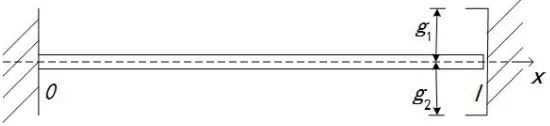
In this paper, we investigate the mechanical behavior of thermoelastic Timoshenko homogeneous
beam, of natural lengthl, which may come in contact with two rigid obstacles (see Figure 1). We denote by ϕ=ϕ(x, t), ψ=ψ(x, t), θ=θ(x, t) and q =q(x, t) the transverse displacement, angle, relative temperature and heat flow, respectively, we consider the following system:
ρ1ϕtt(x, t)−k[ϕx(x, t) +ψ(x, t)]x+αϕt(x, t) = 0, (x, t)∈(0, l)×(0, T),
ρ2ψtt(x, t)−bψxx(x, t) +k[ϕx(x, t) +ψ(x, t)]−mθx(x, t) = 0, (x, t)∈(0, l)×(0, T),
θt(x, t) +rqx(x, t)−mψxt(x, t) = 0, (x, t)∈(0, l)×(0, T), τ qt(x, t) +q(x, t) +rθx(x, t) = 0, (x, t)∈(0, l)×(0, T),
(1.1)
with the initial conditions
ϕ(x,0) =ϕ0(x), ϕt(x,0) =ϕ1(x), x∈[0, l],
and
ϕ(0, t) = 0, ψ(0, t) = 0, q(0, t) = 0, t∈[0, T], (1.3)
ψx(l, t) = 0, θ(l, t) = 0, t∈[0, T], (1.4)
for some given functions ϕ0, ϕ1, ψ0, ψ1, θ0, q0. The coefficients ρ1, ρ2, b, k, α, m and τ represent the mass density, the moment of mass inertia, the rigidity coefficient of cross section, the shear
modulus of elasticity, the coefficient of the damping force, the coupling coefficient depending on
the material properties and the thermal diffusivity, respectively, with ρ1, ρ2, k, b, τ, α ∈ R+ and m∈R\ {0}.
Figure 1: A thermoelastic Timoshenko beam and the tip at x=l with clearanceg=g1+g2.
The tip at x = l is modeled with the Signorini non-penetration condition, see [21, 28]. In particular, the tip with gap g is the asymmetrical so that g=g1+g2, where g1 >0 and g2 >0
are, respectively, the upper and lower clearances, when the system is at rest (see Figure 1). Then,
the right end of the beam is assumed to move vertically only between two stops, namely
−g2 ≤ϕ(l, t)≤g1, t∈(0, T). (1.5)
We denote by σ(t) the shear stress at x=l, i.e.,
σ(t) :=k[ϕx(l, t) +ψ(l, t)].
We require that when there is no contact, namely −g2 < ϕ(l, t) < g1, the right end is free and σ(t) = 0. On the other hand, when u(l, t) is in contact, namely ϕ(l, t) = −g2 or ϕ(l, t) = g1, the stress is opposite to the displacement: σ(t) ≥0 if ϕ(l, t) =−g2 and σ(t)≤ 0 ifϕ(l, t) =g1.
Accordingly, we prescribe
−σ(t)∈∂X(ϕ(l, t)), t∈[0, T], (1.6)
where∂X denotes the subdifferential of the indicator function X
X(ϕ) = (
0, if −g2< ϕ < g1,
+∞, otherwise,
namely
∂X(ϕ) =
(−∞,0], if ϕ=−g2,
0, if −g2< ϕ < g1,
Many researchers got interested in studying the dynamics contact problems involving only a
single displacement and/or a single variation of temperature, see for example [2, 3, 21, 22, 28,
38, 44]. Carlson [12] and Day [18] found that two or more materials may come in contact as a
result of thermoelastic expansion or contraction in industrial processes. Copetti [15], Kuttler and
Shillor [27] proposed the dynamic evolution of a thermoviscoelastic rod which may contact or
impact a rigid or reactive obstacle, whereas the exponential energy decay rate for weak solutions
of a thermoelastic rod, contacting a rigid obstacle, has been analyzed in [36]. Copetti [16] proved
existence and uniqueness results and proposed finite element approximations in space with
back-ward Euler discretization in time for a contact problem in generalized thermoelasticity under the
theory of thermoelasticity proposed by Green and Lindsay [24]. Berti and Naso [10] considered
the existence and longtime behavior of solutions for a dynamic contact problem between a
non-linear viscoelastic beam and two rigid obstacles. Afterward, thermal effects have been also taken
into account in [7, 9], where Berti et al. proved the existence and uniqueness of the solution as
well as the exponential decay of the related energy.
Timoshenko beam with thermal contribution have been investigated by many authors and
some results related to global existence and decay properties have been obtained, see for example
[13, 14, 19, 20, 23, 25, 29, 32, 35, 43, 46]. For the case of nonlinear internal frictional damping and
without thermal effects, we refer the readers to Boussouira [1], Rivera and Racke [37], Raposo
et al. [42] and Soufyane [45]. The boundary stabilization and boundary control have been
studied in [26, 48] (see also references therein). Arantes and Rivera in [5] proved that the energy
associated with the thermoelastic Timoshenko beam system decays exponentially as time goes
to infinity. Meanwhile, a great number of researchers have devoted considerable amount time
studying Timoshenko beam with contact problems. For instances, in [6], Araruna et al. showed the
existence of solutions and the exponential stability of the energy for a contact problem associated
with an elastic Timoshenko beam and a rigid obstacle under the assumption of a dissipative
boundary feedback. Berti et al. [8] proved global existence in time of solutions and exponential
decay for a dynamic contact problem between a Timoshenko beam and two rigid obstacles. In
[17], well-posedness and fully discrete approximations for a dynamic contact problem between a
viscoelastic Timoshenko beam and a deformable obstacle was analyzed.
In the above-mentioned result of Berti et al. [8], the heat dissipation is given through Fourier’s
law. As it is well known, by using the Fouriers law for the heat conduction, the thermal effect
is propagated in an infinite speed in thermoelasticity. To overcome this physical paradox, many
theories have been developed. Lord and Shulman [31] suggested that Fouriers law was replaced
by Cattaneos law to describe the heat conduction, which transforms the classical thermoelastic
system into the thermoelastic system with second sound, in which the thermal disturbance is
propagated in a finite speed. Over the past decade, sevaral asymptotic behavior results have been
obtained for the thermoelasticity system with second sound ([4, 11, 30, 33, 34, 39, 40, 41, 47]).
Berti et al. [9] investigated a dynamic contact problem describing the mechanical and thermal
Motivated by these results, the aim of the present paper is to establish a global in time
existence result to problem (1.1)-(1.6) and analyze its longtime behavior. In particular, we prove
that the system possesses an energy decaying exponentially as time goes to infinity. Problem
(1.1)-(1.6) can be regarded as an extension and improvement of Berti et al. [8] to the thermoelastic
Timoshenko beam with second sound. It has been shown in [23] that the dissipative effects of heat
conduction induced by Cattaneo’s law are usually weaker than those induced by Fourier’s law,
and the coupling via Cattaneo’s law may cause loss of the exponential decay usually obtained in
the case of coupling via Fouriers law. The main difficulties also arise from the irregular boundary
terms induced by the constraint (1.6) and from the low regularity of the weak solution. In order
to prove the global existence result, we consider an approximate version of problem (1.1)-(1.6) by
introducing a normal compliance condition as regularization of the Signorini condition (1.6). We
first prove a well-posedness result for the penalized problem by means of a Faedo-Galerkin scheme,
and then derive suitable a priori estimates and pass to the limit in the regularization parameter
obtaining the existence of a solution to the original problem. In order to get the exponential
decay result to problem (1.1)-(1.6), we consider the approximate framework. By introducing a
suitable Lyapunov functional and using the multiplier method, we first obtain the exponential
decay result for the approximate solution. Then, under weak lower semicontinuity arguments, we
prove the exponential decay rate for a solution to the original problem.
The paper is organized as follows. In Section 2, a variational formulation of problem (1.1)-(1.6)
has been introduced and the main results have been stated. In Section 3, we study the existence
of a weak solution to problem (1.1)-(1.6). The exponential stability result is proved in Section 4.
2
Main results
To give a variational formulation of the problem, we introduce the following spaces:
V=f ∈H1(0, l) : f(0) = 0 , K={ϕ∈ V : −g2 ≤ϕ(l)≤g1}, H=
f ∈H1(0, l) : f(l) = 0 .
The initial data
(ϕ0, ψ0, θ0, q0)∈ K × V ×L2(0, l)×L2(0, l), (ϕ1, ψ1)∈[L2(0, l)]2. (2.1) We define
E(t) :=E(t, ϕ, ψ, θ, q) =1 2
Z l
0
ρ1|ϕt(x, t)|2+ρ2|ψt(x, t)|2+|θ(x, t)|2+τ|q(x, t)|2 +k|ϕx(x, t) +ψ(x, t)|2+b|ψx(x, t)|2
dx (2.2)
Definition 2.1 Let ϕ0, ψ0, θ0, q0, ϕ1, ψ1 be given as in (2.1) and 0 < T ≤ ∞. We say that
(ϕ, ψ, θ, q) is a weak solution to problem (1.1)-(1.6) when
ϕ∈W1,∞(0, T;L2(0, l))∩L∞(0, T;K), ψ∈W1,∞(0, T;L2(0, l))∩L∞(0, T;V), θ∈L∞(0, T;L2(0, l)),
q∈L∞(0, T;L2(0, l)),
with initial data satisfying (1.2), the inequality
Z T
0
Z l
0
{−ρ1ϕt(x, t)[ωt(x, t)−ϕt(x, t)] +k[ϕx(x, t) +ψ(x, t)][ωx(x, t)−ϕx(x, t)]
+αϕt(x, t)[ω(x, t)−ϕ(x, t)]}dxdt≥ρ1
Z l
0
ϕ1(x)[ω(x,0)−ϕ0(x)]dx, (2.3)
for everyω ∈W1,1(0, T;L2(0, l))∩L2(0, T;K) such that ω(·, T) =ϕ(·, T), and the equations Z T
0
Z l
0
{−ρ2ψt(x, t)Xt(x, t) +bψxXx(x, t) +k[ϕx(x, t) +ψ(x, t)]X(x, t)
+mθ(x, t)Xx(x, t)}dxdt=ρ2
Z l
0
ψ1(x)X(x,0)dx, (2.4)
Z T
0
Z l
0
{−θ(x, t)nt(x, t)−rqε(x, t)nεx(x, t) +mψxnt(x, t)}dxdt
= Z l
0
[θ(x,0)−mψx(x,0)]n(x,0)dx, (2.5)
Z T
0
Z l
0
{−τ q(x, t)yt(x, t) +qε(x, t)y(x, t) +rθx(x, t)y(x, t)}dxdt
= Z l
0
τ q(x,0)y(x,0)dx, (2.6)
for every X ∈ W1,1(0, T;L2(0, l)) ∩ L2(0, T;V) such that X(·, T) = ψ(·, T), for every n ∈ W1,1(0, T;L2(0, l)∩L2(0, T;H)) and y ∈W1,1(0, T;L2(0, l)∩L2(0, T;V)) such that y(·, T) = 0,
n(·, T) = 0.
Here are the main results of the paper.
Theorem 2.2 (Global existence) Under assumption (2.1), there exists a weak solution (in the
sense of Definition 2.1) of problem (1.1)-(1.6).
By a regularization, a priori estimates, and passage to the limit procedure, the proof of this
result will be carried out in Section 3. In Section 4, we shall prove the following exponential decay
result.
Theorem 2.3 (Exponential decay) Let ϕ be a weak solution to problem (1.1)-(1.6) provided by Theorem 2.2. Then there exist two positive constants R andω, independent of t, such that
3
Global existence
In this section, we show that the solution for problem (1.1)-(1.6) is global. Firstly, in Section 3.1,
we approximate problem (1.1)-(1.6) by a penalization procedure and we prove well-posedness for
the regularized problem (Proposition 3.1 below). Then, in Section 3.2, we show that a sequence
of approximate solutions converges to a solution to the original problem.
3.1 Approximating problem
For anyε >0, we introduce the families of initial data (ϕε
0, ψε0, θε0, qε0)ε>0, satisfying
(ϕε0, ψ0ε, θ0ε, q0ε)∈[H2(0, l)∩ K]×[H2(0, l)∩ V]× H × V, (ϕε1, ψ1)ε∈[H1(0, l)]2. (3.1)
We introduce a penalized version of problem (1.1)-(1.6) by regularizing the Signorini contact
condition with a normal compliance condition. We consider the following system:
ρ1ϕεtt(x, t)−k[ϕεx(x, t) +ψε(x, t)]x+αϕεt(x, t) = 0, (x, t)∈(0, l)×(0, T), ρ2ψεtt(x, t)−bψxxε (x, t) +k[ϕεx(x, t) +ψε(x, t)]−mθεx(x, t) = 0, (x, t)∈(0, l)×(0, T),
θεt(x, t) +rqxε(x, t)−mψεxt(x, t) = 0, (x, t)∈(0, l)×(0, T), τ qεt(x, t) +qε(x, t) +rθxε(x, t) = 0, (x, t)∈(0, l)×(0, T),
(3.2)
together with
ϕε(x,0) =ϕε0(x), ϕεt(x,0) =ϕε1(x), x∈[0, l], ψε(x,0) =ψ0ε(x), ψtε(x,0) =ψε1(x), x∈[0, l], θε(x,0) =θε
0(x), qε(x,0) =q0ε(x), x∈[0, l].
(3.3)
The boundary conditions at x= 0 are
ϕε(0, t) = 0, ψε(0, t) = 0, qε(0, t) = 0, t∈[0, T]. (3.4)
At the tipx=l, fort∈[0, T], we set
ψxε(l, t) = 0, θε(l, t) = 0, σε(t) = ˜σε(t), (3.5)
where
σε(t) =k[ϕxε(l, t) +ψε(l, t)],
˜
σε(t) =−1 ε
[ϕε(l, t)−g1]+−[−ϕε(l, t)−g2]+ −εϕεt(l, t). (3.6) Here and in the sequel, [f]+:= max{f,0}denotes the positive part of a function f.
Henceforth, we will also use the following functionals:
Jε(t) = 1 2ε
|[ϕε(l, t)−g1]+|2+|[−ϕε(l, t)−g2]+|2 , (3.7)
Eε(t) =Eε(t) +Jε(t), (3.8)
Proposition 3.1 (Existence of an approximate solution) Given any T >0, problem (3.2)has a solution
ϕn,ε∈W2,∞(0, T;L2(0, l))∩W1,∞(0, T;H1(0, l))∩L∞(0, T;H2(0, l)), ψn,ε ∈W2,∞(0, T;L2(0, l))∩W1,∞(0, T;H1(0, l))∩L∞(0, T;H2(0, l)), θn,ε ∈W1,∞(0, T;L2(0, l))∩L∞(0, T;H1(0, l)),
qn,ε∈W1,∞(0, T;L2(0, l))∩L∞(0, T;H1(0, l)),
(3.9)
with initial data satisfying (3.1), (3.3) and compatible with the boundary conditions (3.4)-(3.6)
fort= 0.
Proof. (Construction of Faedo-Galerkin approximations) Let {wj}∞
j=1, be a basis of V and {ξj}∞j=1 is basis ofH such thatw1 =ϕε0, w2 =ϕε1, w3 =ψ0ε, w4 =ψε1, w5 =q0ε and ξ1 =θ0ε.We
construct the approximate solutions of the form
ϕn,ε(x, t) = n X
j=1
hnj(t)wj(x), ψn,ε(x, t) = n X
j=1
pnj(t)wj(x),
θn,ε(x, t) = n X
j=1
unj(t)ξj(x), qn,ε(x, t) = n X
j=1
vjn(t)wj(x),
verifying, for j= 1, ..., n,
Z l
0
{ρ1ϕn,εtt (x, t)wj(x) +k[ϕn,εx (x, t) +ψn,ε(x, t)]wjx(x) +αϕn,εt (x, t)wj(x)}dx
−σ˜n,ε(t)wj(l) = 0, (3.10)
Z l
0
{ρ2ψttn,ε(x, t)wj(x) +bψxn,ε(x, t)wjx(x) +k[ϕn,εx (x, t) +ψn,ε(x, t)]wj(x)
−mθn,εx (x, t)wj(x)}dx= 0, (3.11)
Z l
0
[θn,εt (x, t)ξj(x)−rqn,ε(x, t)ξjx(x) +mψtn,ε(x, t)ξjx(x)] dx= 0, (3.12)
Z l
0
[τ qn,εt (x, t)wj(x) +qn,ε(x, t)wj(x)−rθn,ε(x, t)wjx(x)] dx= 0, (3.13)
where
˜
σn,ε(t) =−1 ε
[ϕn,ε(l, t)−g1]+−[−ϕn,ε(l, t)−g2]+ −εϕn,εt (l, t) and initial data
ϕn,ε(x,0) =ϕε0(x), ϕn,εt (x,0) =ϕε1(x), x∈[0, l], ψn,ε(x,0) =ψ0ε(x), ψn,εt (x,0) =ψ1ε(x), x∈[0, l], θn,ε(x,0) =θε0(x), qn,ε(x,0) =q0ε(x), x∈[0, l].
(3.14)
Accordingly, the standard theory of ordinary differential equations guarantees, under Lipschitz
now need the a priori estimates that permit us to extend the solution to the whole interval [0, T],
for any T >0.
(A priori estimates) We multiply (3.10) by hnjt, (3.11) by pnjt, (3.12) by unj, (3.13) by vnj, respectively, summing over j and adding the resulting equations, we infer
d dtE
n,ε(t) +α Z l
0
|ϕn,εt (x, t)|2dx+
Z l
0
|qn,ε(x, t)|2dx= ˜σn,ε(t)ϕn,ε t (l, t),
whereEn,ε(t) =E(t, ϕn,ε, ψn,ε, θn,ε, qn,ε).Note that if we denote byf− = max{−f,0}the negative part of a function f, we have f+ft = f+(f+−f−)t = f+ft+ =
1 2
d dt[f
+]2. Thus, the previous
equality becomes
d dtE
n,ε(t) +α Z l
0
|ϕn,εt (x, t)|2dx+ Z l
0
|qn,ε(x, t)|2dx+ε|ϕn,εt (l, t)|2 = 0.
An integration over (0, t) and initial conditions (3.14) ensure that
En,ε(t) + 1 2ε
|[ϕn,ε(l, t)−g1]+|2+|[−ϕn,ε(l, t)−g2]+|2 ≤K, (3.15)
whereK is a positive constant independent ofn. Note that for anyϕε0∈ K we get that ˜σn,ε(0) =
−εϕn,εt (l,0).
After a differentiation of Eqs. (3.10)-(3.13) with respect to t, we have
Z l
0
{ρ1ϕn,εttt(x, t)wj(x) +k[ϕn,εxt (x, t) +ψ n,ε
t (x, t)]wjx(x) +αϕ n,ε
tt (x, t)wj(x)}dx
−σ˜n,εt (t)wj(l) = 0, (3.16)
Z l
0
{ρ2ψtttn,ε(x, t)wj(x) +bψxtn,ε(x, t)wjx(x) +k[ϕn,εxt(x, t) +ψ n,ε
t (x, t)]wj(x)
−mθn,εxt (x, t)wj(x)}dx= 0, (3.17)
Z l
0
[θn,εtt (x, t)ξj(x)−rqn,εt (x, t)ξjx(x) +mψttn,ε(x, t)ξjx(x)] dx= 0, (3.18)
Z l
0
[τ qn,εtt (x, t)wj(x) +qtn,ε(x, t)wj(x)−rθn,εt (x, t)wjx(x)] dx= 0. (3.19)
We multiply (3.16) by hn
jtt, (3.17) by pnjtt, (3.18) by unjt, (3.19) by vjtn, summing over j and adding the resulting equations, we have
d dtE
n,ε t (t) +α
Z l
0
|ϕn,εtt (x, t)|2dx+ Z l
0
|qtn,ε(x, t)|2dx+ε|ϕn,εtt (l, t)|2 =−1 εB
n(t)ϕn,ε
tt (l, t), (3.20)
whereEtn,ε(t) =E(t, ϕn,εt , ψn,εt , θtn,ε, qtn,ε) and Etn,ε(t) , Bn(t) are defined as follows
Etn,ε(t) :=1 2
Z l
0
+1 2
Z l
0
k|ϕn,εxt (x, t) +ψtn,ε(x, t)|2+τ|qtn,ε(x, t)|2+|θn,εt (x, t)|2 dx,
Bn(t) =d dt
[ϕn,ε(l, t)−g1]+−[−ϕn,ε(l, t)−g2]+ .
In addition, by applying the Young’s and Sobolev’s inequalities and noting that|(f+)t| ≤ |ft|, we can estimate the last term in (3.20) as follows (see [8])
1
ε|B
n(t)||ϕn,ε tt (l, t)|
≤ε
2|ϕ n,ε
tt (l, t)|2+Cε|Bn(t)|2
≤ε
2|ϕ n,ε tt (l, t)|
2+C
ε Z l
0
|ϕn,εxt (x, t) +ψn,εt (x, t)|2dx+Cε Z l
0
|ψxtn,ε(x, t)|2dx,
where Cε is a positive constant depending on ε but independent of n, which is allowed to vary even in the same formula. From (3.20), we have
d dtE
n,ε t (t) +α
Z l
0
|ϕn,εtt (x, t)|2dx+ Z l
0
|qn,εt (x, t)|2dx+ ε 2|ϕ
n,ε tt (l, t)|2
≤Cε
Z l
0
|ϕn,εxt (x, t) +ψtn,ε(x, t)|2dx+C
ε Z l
0
|ψxtn,ε(x, t)|2dx. (3.21)
An integration over (0, t) implies
Etn,ε(t) + Z t
0
Z l
0
α|ϕn,εtt (x, t)|2+|qn,ε t (x, t)|2
dxdt
≤Etn,ε(0) +Cε Z t
0
Z l
0
|ϕn,εxt (x, t) +ψn,εt (x, t)|2+|ψxtn,ε(x, t)|2
dxdt. (3.22)
We can show that the second order energy is initially bounded, independently of n, namely
Etn,ε(0) :=1 2
Z l
0
ρ1|ϕn,εtt (x,0)|2+ρ2|ψttn,ε(x,0)|2+|θ n,ε
t (x,0)|2+τ|q n,ε t (x,0)|2
dx +1 2 Z l 0
k|ϕn,ε1x(x) +ψn,ε1 (x)|2+b|ψ1n,εx(x)|2 dx
is bounded independently ofn. To this aim, we multiply (3.10) byhnjtt, we sum up overj= 1, ..., n
and we let t→0. By (3.14), we have
Z l
0
ρ1|ϕn,εtt (x,0)|2+k[ϕε0x(x) +ψε0(x)]ϕ
n,ε
xtt(x,0) +αϕε1(x)ϕ
n,ε
tt (x,0) dx
−σ˜n,ε(0)ϕn,εtt (l,0) = 0.
After an integration by parts and owing to the compatibility conditions (3.4)-(3.6) fort= 0, we find
Z l
0
ρ1|ϕn,εtt (x,0)|
2−k[ϕε
0xx(x) +ψε0x(x)]ϕ n,ε
tt (x,0) +αϕ ε
1(x)ϕ
n,ε
tt (x,0) dx
In the light of H¨older’s inequality and Young’s inequality, we deduce that there exists a constant
C independent of nsuch that
Z l
0
|ϕn,εtt (x,0)|2dx≤C
Z l
0
[|ϕε0xx(x)|2+|ψ0εx(x)|2+|ϕε1(x)|2]dx≤C.
Similarly, multiplying (3.11) bypnjtt, (3.12) byunjt, summing up overj= 1, ..., nand lettingt→0, we get
Z l
0
|ψn,εtt (x,0)|2dx≤C
Z l
0
[|ψ0εxx(x)|2+|ϕε0x(x)|2+|θε0x(x)|2]dx≤C
and
Z l
0
|θtn,ε(x,0)|2+rqε0x(x)θn,εt (x,0)−mψε1x(x)θn,εt (x,0) dx= 0,
which leads to the inequality
Z l
0
|θn,εt (x,0)|2dx≤C
Z l
0
[|qε0x(x)|2+|ψ1εx(x)|2]dx≤C.
Finally, multiplying (3.13) byvjtn, summing up over j= 1, ..., nand letting t→0, we obtain
Z l
0
τ|qn,εt (x,0)|2+qn,ε
0 (x)q
n,ε
t (x)−rθ n,ε
0xq n,ε
t (x,0) dx= 0,
then, we have
Z l
0
|qn,εt (x,0)|2dx≤C
Z l
0
[|qε
0(x)|2+|θε0x(x)|2]dx≤C. By (3.1), we infer that
Etn,ε(0)≤C
Z l
0
|ϕε
0xx(x)|2+|ψ0εxx(x)|2+|θε0x(x)|2+|qε0(x)|2+|ϕε1(x)|2+|ψε1x(x)|2
dx≤C.
Thus, from (3.22) and applying Gronwall’s inequality, we find thatEtn,ε(t) is bounded in [0, T]. (Passage to the limit) Inequalities (3.15) and (3.22) guarantee that
ϕn,ε is bounded in W2,∞(0, T;L2(0, l))∩W1,∞(0, T;H1(0, l)), ψn,ε is bounded in W2,∞(0, T;L2(0, l))∩W1,∞(0, T;H1(0, l)), θn,ε is bounded in W1,∞(0, T;L2(0, l)), qn,ε is bounded in W1,∞(0, T;L2(0, l)),
[ϕn,ε(l, t)−g1]+ is bounded inL∞(0, T),
[−ϕn,ε(l, t)−g2]+ is bounded inL∞(0, T).
Therefore we deduce, up to a subsequence, the convergence
ψn,ε* ψε weak∗ inW2,∞(0, T;L2(0, l))∩W1,∞(0, T;H1(0, l)), θn,ε* θε weak∗ inW1,∞(0, T;L2(0, l)), qn,ε* qε weak∗ inW1,∞(0, T;L2(0, l)),
[ϕn,ε(l, t)−g1]+*[ϕε(l, t)−g1]+ weak∗ inL∞(0, T),
[−ϕn,ε(l, t)−g2]+*[−ϕn,ε(l, t)−g2]+ weak∗ inL∞(0, T).
By standard procedure, by lettingn→ ∞in (3.10), we recover (3.2) and the initial and boundary conditions (3.3)-(3.6). In particular, from equations (3.2)3 and (3.2)4, we deduce that θxε, qεx ∈ L∞(0, T;L2(0, l)) and hence the regularity (ϕε, ψε, θε, qε) verifies the regularity specified in (3.9). Proposition 3.2 (Uniqueness) For anyT >0, the solution(ϕε, ψε, θε, qε) to problem (3.2), with initial data satisfying (3.3)and compatible with the boundary conditions (3.4)-(3.6), is unique.
Proof. Let (ϕε, ψε, θε, qε) and (Φε,Ψε,Θε,Υε) be two solutions of (3.2), (3.4)-(3.6) whose regu-larity is specified by (3.9). We define
Uε :=ϕε−Φε, Qε:ψε−Ψε, Rε:=θε−Θε, Sε:=qε−Υε,
satisfying
ρ1Uttε(x, t)−k[Uxε(x, t) +Qε(x, t)]x+αUtε(x, t) = 0, (x, t)∈(0, l)×(0, T), ρ2Qεtt(x, t)−bQεxx(x, t) +k[Uxε(x, t) +Qε(x, t)]−mRxε(x, t) = 0, (x, t)∈(0, l)×(0, T),
Rεt(x, t) +rSxε(x, t)−mQεxt(x, t) = 0, (x, t)∈(0, l)×(0, T), τ Stε(x, t) +Sε(x, t) +rRεx(x, t) = 0, (x, t)∈(0, l)×(0, T),
with the initial conditions
Uε(x,0) = 0, Utε(x,0) = 0, x∈[0, l], Qε(x,0) = 0, Qεt(x,0) = 0, x∈[0, l], Rε(x,0) = 0, Sε(x,0) = 0, x∈[0, l]
(3.23)
and
Uε(0, t) = 0, Qεt(0, t) = 0, Rε(0, t) = 0, Sε(0, t) = 0, (3.24)
Qε(l, t) =Qεx(l, t) = 0, Rε(l, t) = 0, Sε(l, t) = 0, ςε(t) = ˜ςε(t), t∈[0, T], (3.25)
where
ςε(t) =k[Uxε(l, t) +Qε(l, t)],
˜
ςε(t) =−1 ε
[ϕε(l, t)−g1]+−[−ϕε(l, t)−g2]+−[Φε(l, t)−g1]++ [−Φε(l, t)−g2]+ −εUtε(l, t).
Multiplying (3.16) by Utε, (3.17) by Qεt, (3.18) byRε, (3.19) by Sε and integrating over [0, l], we get
d
dtE(t,(U
ε, Qε, Rε, Sε)) +α Z l
0
|Utε(x, t)|2dx+ Z l
0
In view of the relation|f+−g+| ≤ |f−g|, we obtain the estimate
[ϕε(l, t)−g1]+−[−ϕε(l, t)−g2]++ [Φε(l, t)−g1]+−[−Φε(l, t)−g2]+
≤2|ϕε(l, t)−Φε(l, t)|= 2|Uε(l, t)|.
By means of Poincar´e’s inequality and the Sobolev embedding theorem, we have
˜
ςε(t)Utε(l, t) =−1 ε
[ϕε(l, t)−g1]+−[−ϕε(l, t)−g2]+−[Φε(l, t)−g1]+
+[−Φε(l, t)−g2]+ Utε(l, t)−ε|Utε(l, t)|2
≤2 ε|U
ε(l, t)||Uε
t(l, t)| −ε|Utε(l, t)|2
≤ −ε
2|U ε
t(l, t)|2+Cε|Uε(l, t)|2
≤ −ε
2|U ε
t(l, t)|2+Cε Z l
0
|Uxε(x, t)|2dx.
A substitution into (3.26) leads to
d dtE(t, U
ε, Qε, Rε, Sε) +α Z l
0
|Utε(x, t)|2dx+ Z l
0
|Sε(x, t)|2dx+ε 2|U
ε
t(l, t)|2≤CEε(t). In view of initial conditions (3.23)-(3.25), E(0, Uε, Qε, Rε, Sε) = 0. Thus, by the Gronwall lemma, we find that E(t, Uε, Qε, Rε, Sε) = 0 on [0, T]. This implies that (ϕε, ψε, θε, qε) = (Φε,Ψε,Θε,Υε), and our conclusion follows.
3.2 Proof of Theorem 2.2
The idea is to consider a sequence of approximate solutions (provided by Proposition 3.1) and
to show their convergence (as ε → 0) to a weak solution of problem (1.1)-(1.6). Given data (ϕε0, ψ0ε, θ0ε, q0ε)∈ K × V ×L2(0, l)×L2(0, l), (ϕ1, ψ1)∈[L2(0, l)]2, let us consider the sequences of functions (ϕε0, ψε0, θε0, q0ε), (ϕε1, ψε1) with the regularity expressed in (3.1) and such that
(ϕε0, ψε0, θ0ε, q0ε)→(ϕ0, ψ0, θ0, q0)∈ V × V ×L2(0, l)×L2(0, l),
(ϕε
1, ψε1)→(ϕ1, ψ1)∈ [L2(0, l)]2.
(3.27)
Multiplying equations (3.2)1, (3.2)2, (3.2)3, (3.2)4, byϕtε,ψεt,θε,qεand summing up the resulting equations. An integration over (0, l) and boundary conditions (3.4)-(3.6) lead to
d dtE
ε(t) +α Z l
0
|ϕεt(x, t)|2dx+ Z l
0
|qε(x, t)|2dx+ε|ϕεt(l, t)|2= 0, (3.28) where the functionalEε is defined in (3.8). Now we integrate overt, by (3.1)
1 and Jε(0) = 0,we
have
Eε(t) + Z t
0
α
Z l
0 |ϕε
t(x, s)|2dx+ Z l
0
|qε(x, s)|2dx+ε|ϕε t(l, s)|2
ds≤Eε(0)≤K, (3.29)
whereK is a positive constant independent ofε. By (3.29), we obtain the estimate
Jε(t) = 1 2ε
The boundedness ofEε(t) implies the existence of a subsequence, we get
ϕε* ϕ weak∗ in W1,∞(0, T;L2(0, l))∩L∞(0, T;H1(0, l)), ψε* ψ weak∗ inW1,∞(0, T;L2(0, l))∩L∞(0, T;H1(0, l)), θε* θ weak∗ inL∞(0, T;L2(0, l)),
qε * q weak∗ inL∞(0, T;L2(0, l)).
(3.31)
Moreover, we have
εϕεt(l,·)→0 inL2(0, T). (3.32)
Next, we will prove that (ϕ, ψ, θ, q) is a weak solution to problem (1.1)-(1.6). Inequality (3.30) assures that ϕ(·, t) ∈ K for all t ∈ [0, T]. Now, let ω ∈ W1,1(0, T;L2(0, l))∩L2(0, T;K) such that ω(·, T) =ϕ(·, T). Multiplying (3.2)1 by ω−ϕε and integrate over (0, T)×(0, l). By taking (3.5)-(3.6) into account, we obtain
Z T
0
Z l
0
{−ρ1ϕεt(x, t)[ωt(x, t)−ϕεt(x, t)] +k[ϕεx(x, t) +ψε(x, t)][ωx(x, t)−ϕεx(x, t)]
+αϕεt(x, t)[ω(x, t)−ϕε(x, t)]}dxdt≥ρ1
Z l
0
ϕε1(x)[ω(x,0)−ϕε0(x)]dx.
Similarly, from (3.2)2, (3.2)3 and (3.2)4, we have Z T
0
Z l
0
{−ρ2ψεt(x, t)Xt(x, t) +bψxεXx(x, t) +k[ϕεx(x, t) +ψε(x, t)]X(x, t)
+mθε(x, t)Xx(x, t)}dxdt=ρ2
Z l
0
ψε1(x)X(x,0)dx,
Z T
0
Z l
0
{−θε(x, t)nt(x, t)−rqε(x, t)nεx(x, t) +mψεxnt(x, t)}dxdt
= Z l
0
[θε(x,0)−mψxε(x,0)]n(x,0)dx,
Z T
0
Z l
0
{−τ qε(x, t)yt(x, t) +qε(x, t)y(x, t) +rθεx(x, t)y(x, t)}dxdt
= Z l
0
τ qε(x,0)y(x,0)dx,
for every X ∈ W1,1(0, T;L2(0, l))∩L2(0, T;V) such that X(·, T) = 0, for every n ∈ W1,1(0, T;
L2(0, l))∩L2(0, T;H)) such thatn(·, T) = 0 and for every y ∈W1,1(0, T;L2(0, l))∩L2(0, T;V)) such that v(·, T) = 0. Next, we pass to the limit as ε→0 in the previous relations. By [6], one can obtain the relations
lim ε→0sup
Z T
0
Z l
0
= Z T
0
Z l
0
ρ1|ϕεt(x, t)|2−k[ϕεx(x, t) +ψε(x, t)]ϕεx(x, t)−αϕε(x, t)ϕεt(x, t) dxdt,
which allows us to pass to the limit in the nonlinear terms even though the convergences are
only weak. Accordingly, in view of convergences (3.31) and (3.32), we recover (2.3)-(2.6). This
completes the proof.
4
Exponential decay
In this section, we prove an exponentially stability result of system (1.1)-(1.6). We introduce the
following Lyapunov functional:
Lε(t) =Eε(t) +δ1I1ε(t) +δ2I2ε(t) +δ3I3ε(t), (4.1) where
I1ε(t) = Z l
0
[ρ1ϕεt(x, t)ϕε(x, t) +ρ2ψεt(x, t)ψε(x, t)]dx+
α
2 Z t
0
|ϕε(x, t)|2dx+ε
2|ϕ
ε(l, t)|2, (4.2)
I2ε(t) =−
Z l
0 ρ2
Z x
0
θε(y, t)dy
ψεt(x, t)dx, (4.3)
I3ε(t) =−
Z l
0 τ
Z x
0
θε(y, t)dy
qε(x, t)dx, (4.4)
forδ1,δ2,δ3 are positive constants which will be fixed later.
It is easy to check that, by using Young’s inequality, Poincar´e’s inequality and Sobolev
em-bedding theorem, there exist two constantsβ1 and β2 such that
β1Eε(t)≤Lε(t)≤β2Eε(t). (4.5)
Next, we estimate the derivative ofLε(t) according to the following lemmas.
Lemma 4.1 Let (ϕε, ψε, θε, qε) be the solution provided by Proposition 3.1. Then there holds
d dtI
ε
1(t)≤ρ1
Z l
0 |ϕε
t(x, t)|2dx+ρ2
Z l
0 |ψε
t(x, t)|2dx−k Z l
0 |ϕε
x(x, t) +ψε(x, t)|2dx
−(b−mη1)
Z l
0
|ψxε(x, t)|2dx−2Jε(t) + m 4η1
Z l
0
|θε(x, t)|2dx, (4.6)
where Cp is a Poincar´e constant, Jε(t) is defined in (3.7) and η1 is a positive constant to be
chosen later.
Proof. By differentiating (4.2) with respect to tand by means of equation (3.2), we have
d dt
Z l
0
=ρ1
Z l
0
|ϕεt(x, t)|2dx+k
Z l
0
[ϕεx(x, t) +ψε(x, t)]xϕε(x, t)dx−α
2 d dt
Z l
0
|ϕε(x, t)|2dx
+ρ2
Z l
0 |ψε
t(x, t)|2dx+b Z l
0
ψεxx(x, t)ψε(x, t)dx−k
Z l
0
[ϕεx(x, t) +ψε(x, t)]ψε(x, t)dx
+m
Z l
0
θxε(x, t)ψε(x, t)dx.
By H¨older’s inequality and Young’s inequality, we get
d dt
Z l
0
[ρ1ϕεt(x, t)ϕε(x, t) +ρ2ψεt(x, t)ψε(x, t)]dx+α 2
Z l
0
|ϕε(x, t)|2dx
=ρ1
Z l
0
|ϕεt(x, t)|2dx−k
Z l
0
[ϕεx(x, t) +ψε(x, t)]2dx+ρ2
Z l
0
|ψεt(x, t)|2dx
−b
Z l
0
|ψxε(x, t)|2dx+m
Z l
0
θxε(x, t)ψε(x, t)dx+σε(t)ϕε(l, t)
≤ρ1
Z l
0 |ϕε
t(x, t)|2dx−k Z l
0
[ϕεx(x, t) +ψε(x, t)]2dx+ρ2
Z l
0 |ψε
t(x, t)|2dx
−(b−mη1)
Z l
0
|ψεx(x, t)|2dx+ m 4η1
Z l
0
|θε(x, t)|2dx+ ˜σε(t)ϕε(l, t). (4.7) For the last term on the right-hand side of (4.7), we can obtain
˜
σε(t)ϕε(l, t) =−1 ε
[ϕε(l, t)−g1]+−[−ϕε(l, t)−g2]+ ϕε(l, t)−εϕε(l, t)ϕεt(l, t)
≤ − 1 ε[ϕ
ε(l, t)−g
1]+[ϕε(l, t)−g1] +
1
ε[−ϕ
ε(l, t)−g
2]+[ϕε(l, t) +g2] −ε
2 d dt|ϕ
ε(l, t)|2 ≤ − 1
ε
|[ϕε(l, t)−g1]+|2+|[−ϕε(l, t)−g2]+|2
−ε
2 d dt|ϕ
ε(l, t)|2
=−2Jε(t)−ε
2 d dt|ϕ
ε(l, t)|2.
Substituting into the previous inequality, we reach the conclusion.
Lemma 4.2 Let (ϕε, ψε, θε, qε) be the solution provided by Proposition 3.1. Then there holds
d dtI
ε
2(t)≤ − mρ2
2 Z l
0 |ψε
t(x, t)|2dx+kη2
Z l
0 |ϕε
x(x, t) +ψεx(x, t)|2dx +bη2
Z l
0
|ψxε(x, t)|2dx+r
2ρ 2
2m
Z l
0
|qε(x, t)|2dx
+
b
4η2 + lk
4η2 +m
Z l
0
|θε(x, t)|2dx, (4.8)
for a positive constant η2 to be chosen later.
Proof. By using (3.2)-(3.3) and (3.5), we find
d dtI
ε
2(t) =−ρ2
Z l
0
Z x
0
θtε(y, t)dy
ψεt(x, t)dx−ρ2
Z l
0
Z x
0
θε(y, t)dy
=ρ2
Z l
0
Z x
0
rqyε(y, t)dy−
Z x
0
mψyt(y, t)dy
ψεt(x, t)dx−b
Z l
0
Z x
0
θε(y, t)dy
ψxxε (x, t)dx
+k
Z l
0
Z x
0
θε(y, t)dy
[ϕεx(x, t) +ψε(x, t)] dx−m
Z l
0
Z x
0
θε(y, t)
θεx(x, t)dx. (4.9)
We now estimate the right-hand side of (4.9). For a positive constant η2, by Young’s inequality,
we get ρ2 Z l 0 Z x 0
rqyε(y, t)dy−
Z x
0
mψyt(y, t)dy
ψtε(x, t)dx
=rρ2
Z l
0
Z x
0
qyε(y, t)dy
ψεt(x, t)dx−mρ2
Z l
0
Z x
0
ψyt(y, t)dy
ψεt(x, t)dx
≤r 2ρ 2 2m Z l 0
|qε(x, t)|2dx+mρ2 2
Z l
0
|ψtε(x, t)|2dx−mρ2
Z l
0
|ψεt(x, t)|2dx. (4.10)
By H¨older’s inequality, Young’s inequality, Poincar´e’s inequality and (3.4), (3.5), we have
−b
Z l
0
Z x
0
θε(y, t)dy
ψεxx(x, t)dx≤bη2
Z l
0 |ψε
x(x, t)|2dx+
b
4η2
Z l
0
|θε(x, t)|2dx, (4.11)
k
Z l
0
Z x
0
θε(y, t)dy
[ϕεx(x, t) +ψε(x, t)] dx≤kη2
Z l
0
|ϕεx(x, t) +ψε(x, t)|2dx
+ lk 4η2
Z l
0
|θε(x, t)|2dx, (4.12)
−m
Z l
0
Z x
0
θε(y, t)dy
θxεdx=m
Z l
0
|θε(x, t)|2dx. (4.13)
Combining (4.9)-(4.13), we arrive at (4.8).
Lemma 4.3 Let (ϕε, ψε, θε, qε) be the solution provided by Proposition 3.1. Then there holds
d dtI
ε
3(t)≤ −[r−η3l]
Z l
0
|θε(x, t)|2dx+
rτ+mτ 4η3
+ 1
4η3
Z l
0
|qε(x, t)|2dx
+mτ η3
Z l
0
|ψtε(x, t)|2dx, (4.14)
for a positive constant η3 to be chosen later.
Proof. By using (3.2)-(3.3) and (3.5), we find
d dtI
ε
3(t) =−
Z l
0 τ
Z x
0
θεt(y, t)dy
qε(x, t)dx−
Z l
0 τ
Z x
0
θε(y, t)dy
qtε(x, t)dx
=− Z l 0 τ − Z x 0
rqxε(y, t)dy+ Z x
0
mψεxt(y, t)dy
qε(x, t)dx
−
Z l
0
Z x
0
θε(y, t)dy
Integrating by parts, we obtain
d dtI
ε
3(t) =rτ
Z l
0
|qε(x, t)|2dx−mτ
Z l
0
ψtε(x, t)qε(x, t)dx+ Z l
0
Z x
0
θε(y, t)dy
qε(x, t)dx
−r
Z l
0
|θε(x, t)|2dx.
By means of H¨older’s inequality, Young’s inequality, Poincar´e’s inequality, we deduce (4.14).
Proof of Theorem 2.3. From (3.28), (4.6), (4.8) and (4.14), then from (4.1), we obtain
d dtL
ε(t)≤ −[α−δ
1ρ1]
Z l
0
|ϕεt(x, t)|2dx−
δ2mρ2
2 −δ1ρ2−δ3mτ η3 Z l
0
|ψtε(x, t)|2dx
−k[δ1−δ2η2] Z l
0
|ϕεx(x, t) +ψε(x, t)|2dx−[δ1(b−mη1)−δ2bη2] Z l
0
|ψxε(x, t)|2dx
−
δ3(r−η3l)− δ1m
4η1 −δ2
b
4η2 + lk
4η2 +m
Z l
0
|θε(x, t)|2dx
−
1−δ2r 2ρ2
2m −δ3
rτ +mτ 4η3
+ 1
4η3
Z l
0
|qε(x, t)|2dx−2δ1Jε(t)−ε|ϕεt(l, t)|2.
In fact, we first chooseη1< b
2m,η3< r
2l and δ2 <
m
r2ρ2 small enough so that
b−mη1 >0, r−η3l >0,
1−δ2r 2ρ
2
2m >0.
By choosingδ3 < 1 2
rτ+4mτη
3+ 1 4η3
small enough, we have
1−δ2r 2ρ2
2m −δ3
rτ+mτ 4η3 +
1 4η3
>0.
Next, we takeδ1 < ρ1α and η2 < 2δ1δ2 such that
α−δ1ρ1 >0, δ1−δ2η2 >0,
δ1(b−mη1)−δ2bη2>0.
Once δ2, δ3 are fixed, we take δ1 <min
n δ2mρ2
2ρ2 − δ3mτ η3
ρ2 ,
4η1δ3
m (r−η3l)−
4η1δ2 m
b
4η2 + lk
4η2 +m o so that δ2mρ2
2 −δ1ρ2−δ3mτ η3>0,
δ3(r−η3l)−δ1m
4η1 −δ2
b
4η2 + lk
4η2 +m
>0,
combined withδ1< ρ1α, we can obtain
δ1 <min
α ρ1
,δ2mρ2
2ρ2
− δ3mτ η3 ρ2
,4η1δ3
m (r−η3l)−
4η1δ2 m
b
4η2
+ lk 4η2
+m
Hence, We infer the estimate
d dtL
ε(t)≤ −C0Eε(t)≤ −C0
β2L
ε(t),
with a positive constantC0. By direct integration over (t0, t), we have Lε(t)≤Lε(0)e−
C0
β2t,
which, combined with (4.5) withM = C2
β1 and γ = C0
β2, we can obtain
Eε(t)≤MEε(0)e−γt. (4.15)
By (3.1), we get
Jε(0) = 1 2ε
|[ϕε(l,0)−g1]+|2+|[−ϕε(l,0)]+|2 = 0.
Accordingly, we haveEε(0) =Jε(0) +Eε(0) =Eε(0). In view of (4.15), the inequality
Eε(t)≤ Eε(t)≤MEε(0)e−γt=M Eε(0)e−γt
holds. By passing to lim
ε→0inf and on account of (3.27) and (3.31), we reach the conclusion.
Acknowledgments
This work was supported by the National Natural Science Foundation of China [grant number
11301277], the Natural Science Foundation of Jiangsu Province [grant number BK20151523], the
Six Talent Peaks Project in Jiangsu Province [grant number 2015-XCL-020] and the Qing Lan
Project of Jiangsu Province.
References
[1] F. Alabau-Boussouira, Asymptotic behavior for Timoshenko beams subject to a single
non-linear feedback control, NoDEA Nonnon-linear Differential Equations Appl. 14 (2007), no. 5-6,
643–669.
[2] K. T. Andrews, M. Shillor and S. Wright, On the dynamic vibrations of an elastic beam in
frictional contact with a rigid obstacle, J. Elasticity 42(1996), no. 1, 1–30.
[3] H. Antes and P. D. Panagiotopoulos, The boundary integral approach to static and dynamic
contact problems, International Series of Numerical Mathematics, 108, Birkh¨auser, Basel, 1992.
[4] T. A. Apalara and S. A. Messaoudi, An exponential stability result of a Timoshenko system
with thermoelasticity with second sound and in the presence of delay, Appl. Math. Optim.71
[5] S. Arantes, J. Rivera, Exponential decay for a thermoelastic beam between two stops, Journal
of Thermal Stresses 31(2008), no. 6, 537–556.
[6] F. D. Araruna, A. J. R. Feitosa and M. L. Oliveira, A boundary obstacle problem for the
Mindlin-Timoshenko system, Math. Methods Appl. Sci.32 (2009), no. 6, 738–756.
[7] A. Berti et al., Analysis of dynamic nonlinear thermoviscoelastic beam problems, Nonlinear
Anal. 95(2014), 774–795.
[8] A. Berti, J. E. MuMuMuoz Rivera and M. G. Naso, A contact problem for a thermoelastic
Timoshenko beam, Z. Angew. Math. Phys. 66(2015), no. 4, 1969–1986.
[9] A. Berti et al., A dynamic thermoviscoelastic contact problem with the second sound effect,
J. Math. Anal. Appl. 421(2015), no. 2, 1163–1195.
[10] A. Berti and M. G. Naso, Vibrations of a damped extensible beam between two stops, Evol.
Equ. Control Theory 2 (2013), no. 1, 35–54.
[11] F. Boulanouar and S. Drabla, General boundary stabilization result of memory-type
ther-moelasticity with second sound, Electron. J. Differential Equations 2014(2014), No. 202, 18
pp.
[12] D. E. Carlson, Linear Thermoelasticity, in: Handbuch der Physik, Vol.VIa/2, edited by C.
Truesdell, Spinger, Berlin, 1972.
[13] M. M. Cavalcanti et al., Uniform decay rates for the energy of Timoshenko system with the
arbitrary speeds of propagation and localized nonlinear damping, Z. Angew. Math. Phys. 65
(2014), no. 6, 1189–1206.
[14] M. M. Chen, W. J. Liu and W. C. Zhou, Existence and general stabilization of the
Timo-shenko system of thermo-viscoelasticity of type III with frictional damping and delay terms,
Adv. Nonlinear Anal., Online First. DOI: 10.1515/anona-2016-0085
[15] M. I. M. Copetti, Numerical approximation of dynamic deformations of a thermoviscoelastic
rod against an elastic obstacle, M2AN Math. Model. Numer. Anal.38(2004), no. 4, 691–706.
[16] M. I. M. Copetti, A contact problem in generalized thermoelasticity, Appl. Math. Comput.
218 (2011), no. 5, 2128–2145.
[17] M. I. M. Copetti and J. R. Fern´andez, A dynamic contact problem involving a Timoshenko
beam model, Appl. Numer. Math. 63(2013), 117–128.
[18] W. A. Day, Heat Conduction within Linear Thermoelasticity, 3rd Edition, Pergamon, Oxford,
[19] A. Djebabla and N. Tatar, Exponential stabilization of the Timoshenko system by a
thermo-viscoelastic damping, J. Dyn. Control Syst. 16(2010), no. 2, 189–210.
[20] A. Djebabla and N. Tatar, Stabilization of the Timoshenko beam by thermal effect, Mediterr.
J. Math. 7(2010), no. 3, 373–385.
[21] G. Duvaut and J.-L. Lions,Inequalities in mechanics and physics, translated from the French
by C. W. John, Springer, Berlin, 1976.
[22] C. M. Elliott and Q. Tang, A dynamic contact problem in thermoelasticity, Nonlinear Anal.
23 (1994), no. 7, 883–898.
[23] H. D. Fern´andez Sare and R. Racke, On the stability of damped Timoshenko systems:
Cat-taneo versus Fourier law, Arch. Ration. Mech. Anal. 194 (2009), no. 1, 221–251.
[24] A. E. Green and K. A. Lindsay, Thermoelasticity, J. Elasticity,2 (1972), 1–7.
[25] J.-R. Kang, Asymptotic behavior of the thermoelastic suspension bridge equation with linear
memory, Bound. Value Probl. 2016(2016), no. 206, 18 pp.
[26] J. U. Kim and Y. Renardy, Boundary control of the Timoshenko beam, SIAM J. Control
Optim. 25(1987), no. 6, 1417–1429.
[27] K. L. Kuttler and M. Shillor, A dynamic contact problem in one-dimensional
thermovis-coelasticity, Nonlinear World 2 (1995), no. 3, 355–385.
[28] K. L. Kuttler and M. Shillor, Vibrations of a beam between two stops, Dyn. Contin. Discrete
Impuls. Syst. Ser. B Appl. Algorithms 8 (2001), no. 1, 93–110.
[29] W. J. Liu, K. W. Chen and J. Yu, Existence and general decay for the full von Karman
beam with a thermo-viscoelastic damping, frictional dampings and a delay term, IMA J.
Math. Control Inform., Online First. DOI:10.1093/imamci/dnv056 cite:1+2
[30] W. J. Liu and M. M. Chen, Well-posedness and exponential decay for a porous thermoelastic
system with second sound and a time-varying delay term in the internal feedback, Contin.
Mech. Thermodyn., Online First. DOI: 10.1007/s00161-017-0556-z
[31] H. W. Lord and Y. Shulman, A generalized dynamical theory of thermoelasticity, J. Mech.
Phys. Sol. 15(1967), 299–309.
[32] S. A. Messaoudi and A. Fareh, Energy decay in a Timoshenko-type system of thermoelasticity
of type III with different wave-propagation speeds, Arab. J. Math. (Springer) 2(2013), no. 2,
199–207.
[33] S. A. Messaoudi, M. Pokojovy and B. Said-Houari, Nonlinear damped Timoshenko systems
with second sound—global existence and exponential stability, Math. Methods Appl. Sci. 32
[34] S. A. Messaoudi and B. Said-Houari, Exponential stability in one-dimensional non-linear
thermoelasticity with second sound, Math. Methods Appl. Sci. 28(2005), no. 2, 205–232.
[35] S. A. Messaoudi and B. Said-Houari, Energy decay in a Timoshenko-type system of
ther-moelasticity of type III, J. Math. Anal. Appl. 348 (2008), no. 1, 298–307.
[36] J. E. Mu˜noz Rivera and M. de Lacerda Oliveira, Exponential stability for a contact problem
in thermoelasticity, IMA J. Appl. Math. 58(1997), no. 1, 71–82.
[37] J. E. Mu˜noz Rivera and R. Racke, Global stability for damped Timoshenko systems, Discrete
Contin. Dyn. Syst. 9 (2003), no. 6, 1625–1639.
[38] Y. M. Qin and Z. Y. Ma, Global well-posedness and asymptotic behavior of the solutions to
non-classical thermo(visco)elastic models, Springer, Singapore (2016).
[39] R. Racke, Thermoelasticity with second sound—exponential stability in linear and non-linear
1-d, Math. Methods Appl. Sci. 25(2002), no. 5, 409–441.
[40] R. Racke, Asymptotic behavior of solutions in linear 2- or 3-D thermoelasticity with second
sound, Quart. Appl. Math. 61(2003), no. 2, 315–328.
[41] R. Racke and Y.-G. Wang, Asymptotic behavior of discontinuous solutions to thermoelastic
systems with second sound, Z. Anal. Anwendungen 24(2005), no. 1, 117–135.
[42] C. A. Raposo et al., Exponential stability for the Timoshenko system with two weak
damp-ings, Appl. Math. Lett. 18(2005), no. 5, 535–541.
[43] B. Said-Houari and A. Kasimov, Decay property of Timoshenko system in thermoelasticity,
Math. Methods Appl. Sci. 35 (2012), no. 3, 314–333.
[44] P. Shi and M. Shillor, Uniqueness and stability of the solution to a thermoelastic contact
problem, European J. Appl. Math. 1 (1990), no. 4, 371–387.
[45] A. Soufyane, Exponential stability of the linearized nonuniform Timoshenko beam, Nonlinear
Anal. Real World Appl. 10(2009), no. 2, 1016–1020.
[46] F. Tahamtani, On energy decay of ann-dimensional thermoelasticity system with a nonlinear weak damping, Iran. J. Sci. Technol. Trans. A Sci. 32(2008), no. 1, 45–51.
[47] M. A. Tarabek, On the existence of smooth solutions in one-dimensional nonlinear
thermoe-lasticity with second sound, Quart. Appl. Math. 50(1992), no. 4, 727–742.
[48] Q.-X. Yan, S.-H. Hou and D.-X. Feng, Asymptotic behavior of Timoshenko beam with
dis-sipative boundary feedback, J. Math. Anal. Appl. 269(2002), no. 2, 556–577.
c