H
OUSEHOLD
S
AVING IN THE
UK
James Banks
Sarah Tanner
Copy-edited by Judith Payne
The Institute for Fiscal Studies 7 Ridgmount Street London WC1E 7AE tel. (44) 171 291 4800 fax (44) 171 323 4780 email: [email protected] internet: http//www.ifs.org.uk
© The Institute for Fiscal Studies, October 1999 ISBN 1-873357-93-1
Printed by
The research for this report was produced under the auspices of the IFS Savings Consortium, to whom the authors are grateful for financial assistance and many useful discussions and comments in the series of seminars over the last four years. The members of the IFS Savings Consortium are:
The Association of British Insurers
The Association of Unit Trusts and Investment Funds
The Bank of England
The Bradford and Bingley Building Society
HM Treasury
Inland Revenue
Lloyds TSB
McKinseys
National Savings
Summary ix
1 Introduction 1
2 Official information on saving in the UK 7
2.1 The saving rate 7
2.2 Stocks of wealth 11
3 Economic issues in the analysis of household saving
17
3.1 How much should we save? 18
3.2 Portfolio choice and asset holding 26
3.3 Behavioural issues 29
3.4 Empirical evidence 33
4 Trends in asset ownership, 1978–96 37
4.1 The stakeholder society 37
4.2 Interest-bearing accounts 39
4.3 Stocks and shares 41
4.4 Housing 47
4.5 Life assurance 51
4.6 Financial exclusion 53
Appendix. Asset-ownership rates, 1978–96 57 5 A cross-sectional analysis of financial wealth
holdings in 1997–98
61
5.1 The Financial Research Survey 62
5.2 Who owns what assets 65
5.3 The distribution of financial wealth 70 5.4 Empirical evidence on portfolio choices 75
6 The taxation of saving 84
6.1 The economics of taxing saving 84
6.2 Taxing saving in practice 86
6.3 Conclusions 99
7 Conclusions 102
The gradual shift in responsibility for welfare provision, from the government to individuals, is making household saving and wealth holding a key policy concern. Yet remarkably little is known about how much households save or the forms in which they save. Unlike income or expenditure, there is no official individual or household survey collecting detailed information on saving and wealth holdings on an ongoing basis. This has limited the possible analysis of how saving responds to the incentives created by policy changes.
This report reviews the economics of household saving, the taxation of financial assets in the UK and official sources of information on saving and wealth. It also provides new information on trends in asset holding in the household population over the period 1978–96 and a detailed description of asset and wealth holdings in 1997–98.
The following are among the key results and findings in this report:
• The most recent figures show that total wealth in the UK amounted to £2,720 billion, of which around one-quarter was held in the form of liquid financial assets. The rest was held mainly in housing, pensions and life insurance.
• Some inequality in the distribution of wealth is to be expected, given economic theories of the way households accumulate wealth over their life cycle.
• The 1980s were a period of dramatic change in wealth holdings. In particular, there was a spread in ownership of key assets such as housing, pensions and stocks and shares. The only asset less commonly held now than 20 years ago is life insurance.
• In spite of the proliferation of new savings vehicles, the majority of people still hold the majority of their wealth in conventional forms such as interest-bearing accounts at the bank or building society.
• Most individuals do not typically hold large amounts of financial wealth, and around one-third have no interest-bearing financial assets at all. The median level of wealth held in financial assets (banks, building societies, stocks and shares and mutual funds) is £750. This represents relatively little resources with which to cushion the effects of unanticipated changes in income or spending needs.
• Tax-privileged savings vehicles have been taken up relatively widely, but are held predominantly by wealthier households. The median wealth of TESSA and PEP holders is around 20 times that of the population at large.
Introduction
I propose to introduce a wholly new tax incentive which will reward saving and encourage people to build up a stock of capital.
John Major, Chancellor of the Exchequer, Budget Speech 1990
When half the population have only £200 or less in savings, there is broad agreement that we must do more to encourage savings by everyone.
Gordon Brown, Chancellor of the Exchequer, Budget Speech 1998
Current and past UK governments have expressed concern that the level of household saving is too low. A number of reforms have been implemented, most often in the form of tax incentives for particular savings products, to address this perceived problem. The last few years have seen the introduction of Personal Equity Plans (PEPs, 1987), Personal Private Pensions (1988), Tax-Exempt Special Savings Accounts (TESSAs, 1991) and Individual Savings Accounts (ISAs, 1999), all designed to promote saving.1 This report seeks to inform the ongoing debate on saving by providing a detailed empirical analysis of current levels of wealth held by UK households and documenting recent trends in ownership of the key assets — housing, shares, interest-bearing accounts, pensions and life assurance.
1
First, a few definitional issues. Many people, when they talk about how rich or how wealthy an individual is, are actually referring to their income — that is, the flow of money they receive in a given period. In this report, wealth refers specifically to a stock of resources (held in different forms such as stocks and shares, housing or a pension) that individuals have accumulated in the past. Of course, income and wealth are linked in a number of ways. A stock of wealth accumulated in the past gives rise to a flow of income today in the form of interest and dividend payments.2 Also, wealth must be accumulated out of past income through saving — the flow of resources allocated to wealth accumulation each time period.3 If there were no possibility for saving and hence no wealth, individuals would simply have to spend their current income. When their incomes were high, they would spend a lot; when their incomes fell, they would have to cut their spending. Saving is the mechanism that allows people to defer part of their consumption today in favour of consumption tomorrow, where tomorrow could be next week, next year, retirement or even (in the case of saving for bequests) after death.
The decision to save may be driven by a wide range of motivations; Browning and Lusardi (1996), drawing heavily on Keynes, identify nine possible influences on the decision to save:
• the precautionary motive — to build up a reserve against unforeseen contingencies;
2
Some forms of wealth, such as housing, also generate a flow of consumption benefits that would otherwise need to be paid for out of current income.
3
• the life-cycle motive — to provide for an anticipated future relationship between the income and needs of the individual;
• the intertemporal substitution motive — to enjoy interest and appreciation;
• the improvement motive — to enjoy a gradually increasing expenditure;
• the independence motive — to enjoy a sense of independence and the power to do things, without a clear idea, or definite intention, of specific action;
• the enterprise motive — to secure the masse de manœuvre to carry out speculative business projects;
• the bequest motive — to bequeath a fortune;
• the avarice motive — to satisfy pure miserliness; and
• the down-payment motive — to accumulate deposits to buy cars, houses and other durables.
The first thing to note is that this list maps out a very broad definition of saving. ‘Saving’ encompasses an individual’s decision to put money in a pension (the life-cycle motive), to take out insurance against unemployment or ill health (the precautionary motive), to put money into a savings account for a holiday or washing machine (the down-payment motive) as well as to speculate on the stock market (the intertemporal substitution motive).
total GDP in that year. It also shows how wealth is distributed (or not distributed) across the population: in 1995, the wealthiest 1 per cent of individuals owned nearly one-fifth of all wealth, while the wealthiest 50 per cent of the population owned 92 per cent of wealth. However, the published Inland Revenue figures say a lot about the way the majority of wealth is distributed, but much less about the wealth holdings of the majority of the population, and nothing at all about how the distribution of wealth varies according to characteristics such as age and income. This report intends to redress the balance by presenting evidence on saving and wealth from household and individual surveys. These surveys are unlikely to capture the very wealthiest individuals in the country — who account for a very high proportion of total wealth. We therefore do not look at aggregate wealth in detail. Instead, we are interested mainly in the wealth holdings of the majority of households and individuals.
about saving. As a result, it is not a straightforward issue to predict how much individuals ‘should’ be saving at any one point in time without having information on these other factors. Nevertheless, we draw out two clear implications of the model as crucial to interpreting the evidence presented later and in thinking about government policy designed to encourage saving. First, the life-cycle model is consistent with substantial inequality in saving and wealth, particularly across age groups. Second, a priori, a change in the real post-tax rate of return will have an ambiguous effect on the level of saving. Also in Chapter 3, we discuss models of portfolio choice and their predictions for the form in which individuals will choose to hold their wealth.
This report presents new evidence on household and individual wealth using data from two surveys — the Family Expenditure Survey and the NOP Financial Research Survey. Much of what is presented in Chapters 4 and 5 is simple descriptive analysis, largely because this information is currently missing on saving and wealth (compared with income and consumption, for example). We cannot begin to answer the question of whether households are saving enough before we know more about how much households are currently saving and how this varies with their income and other characteristics. The evidence we present is intended to shed light on these issues.
show that, in spite of more widespread home ownership and share ownership, the bottom of the wealth distribution has a growing number of households with no wealth at all.
Using data from the NOP Financial Research Survey, we present a detailed analysis of the current distribution of wealth across individuals. We show how much (or, rather, how little) financial wealth people typically have and how levels of wealth vary according to key characteristics such as age, income and education. We look at holdings of particular assets, such as interest-bearing accounts and stocks and shares, and at how much of their wealth people choose to hold in these different forms.
Official Information on Saving in the UK
This chapter discusses publicly available information on saving and wealth in the UK. At the aggregate level, information in the National Accounts on personal sector incomes and expenditures yields a measure of the flow of savings, while the Inland Revenue statistics contain information on the distribution of stocks of wealth.
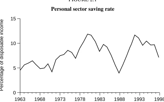
2.1 The Saving Rate
FIGURE 2.1
Personal sector saving rate
1963
Percentage of disposable income
0 15
1998 1968 1973 1978 1983 1988 1993 10
5
Notes: Personal sector saving as a percentage of total resources, which is the sum of gross personal disposable income and the adjustment for the change in net equity of the personal sector in pension funds.
Source: Economic Trends Annual Supplement, 1998, Stationery Office.
premiums, which may be seen as a form of precautionary saving but are in fact classed as expenditure.
More fundamentally, it is not entirely clear what implications should be drawn from looking at the personal sector saving rate.4 Should policymakers be concerned when the personal sector saving rate falls, as it did at the end of the 1980s and as it is doing now? As discussed in more detail in Chapter 3, from a macroeconomic perspective, concern over the rate of saving stems from the fact that savings provide the necessary funds for investment to occur. However, even in a closed economy, it is not just saving by the personal sector that matters for a flow of investment funds, but
4
also saving by the government and the corporate sector. In an open economy such as the UK, international capital flows — not just domestic saving — provide funds for investment. So it is the saving rates of other countries, as well as of the UK, that matter.
From a microeconomic perspective, the concern with a falling personal sector saving rate might be that individuals are not saving enough — to provide for themselves in retirement, for example. In this case, an aggregate measure such as the personal sector saving rate may be relatively uninformative about what is happening to the saving behaviour of most individual households. An aggregate measure will give most weight to the behaviour of the richest households simply as a result of them having a bigger share of total income. Also, a fall in the personal sector saving rate could be the result of changes in the demographic composition of households rather than any underlying behavioural change. For example, an increase in the number of retired people, who are typically net dis-savers, would tend to push down the personal sector saving rate. Rather than looking at an aggregate measure, it may be more useful to look at what has happened over time to the saving rates of different types of households.
fuelled by people borrowing against rising house prices, which in turn were driven by distortions in the housing market. In other words, the growth in consumption was excessive and the fall in saving rate was suboptimal. King (1990) and Pagano (1990) argued that the consumption boom was the result of increased expected future incomes and was entirely consistent with rational, optimising consumer behaviour. This would imply that the fall in saving rate was not a matter for policy concern. Attanasio and Weber (1994) presented evidence that supported this latter view. They found that the consumption boom was greatest among younger cohorts for whom an increase in expected future incomes would translate into a greater increase in anticipated lifetime resources. This difference between younger and older cohorts could not be explained by differences in home-ownership rates.
2.2 Stocks of Wealth
Information on the stock of wealth held by the personal sector is collated by the Inland Revenue from the returns individuals have to make for the purposes of taxing wealth. Unlike income, however, individuals do not have to reveal their entire wealth for tax purposes every year, only when they die. Estimates of personal wealth are constructed from inheritance tax returns using the ‘mortality multiplier method’.5 The estates of those who die each year are grossed up to form an estimate of the wealth of the total population by multiplying each estate by a factor that is, effectively, the inverse of the mortality rate. Clearly, those who die are a non-random group of the population and hence adjustments are made to correct differential mortality by age, gender, marital status and social class. Davies and Shorrocks (1999) argue that those who die are likely to have been in poor health prior to death and been incapable of work and/or incurred larger-than-average expenditures for health and nursing care. For these reasons, the wealth of people who have died may be a poor guide to the wealth of the living, although it is difficult to assess the magnitude of these effects.
Adjustments are made to the initial estimate from the estates information to correct for under-recording and valuation in the estates that are reported and to correct for the fact that not all estates are liable for death duty. Excluded are estates that are too small in total value (currently less than £231,000) and estates passing directly to the surviving spouse. The problem is compounded by the fact that many individuals transfer their wealth before they die in order to reduce their inheritors’ tax liabilities. Of course, such transfers
reduce the size of the tax burden, not the amount of total wealth. This wealth will be picked up in the official estimates to the extent that the recipients of transfers themselves die. But it means that the estimate of total wealth may depend on the very small number of estates of those who die without making transfers. The problem is that the smaller the number of estates on which the estimates of wealth are based, the more unreliable the estimates of total wealth. The adjusted estimates from estates are then reconciled against information from the balance sheets of the financial sector.
Total personal wealth was estimated to be £2,720 billion in 1995 (the latest year for which figures are available) — nearly four times the level of GDP in that year. This represents the value of the stock of individuals’ marketable assets less any amounts due for debts and mortgages. These assets include land and buildings, stocks and shares, trade assets and shares in partnerships, bank and building society deposits, cash, life assurance policies, and cars and other durable goods. The value of occupational and state pensions, however, is not included. This figure for total personal wealth implies a mean level of wealth across the entire adult population of more than £60,000. However, total wealth is distributed unevenly across the adult population. In fact, in 1995, 75 per cent of the adult population were estimated to have £50,000 or under, while 25 per cent of the adult population were estimated to have £5,000 or under.
FIGURE 2.2
Concentration of personal wealth in the UK
1966
Percentage of wealth
0 100
1996 75
50
Top 50%
Top 5%
Top 1%
1966 25
1971 1976 1981 1986 1991
Notes: The measure of wealth is the value of the stock of individuals’ marketable assets less any amounts due for debts and mortgages. The value of occupational and state pensions is not included since the series is not available over the period. Source: Inland Revenue Statistics, 1998, Stationery Office.
of total wealth: in 1995, the wealthiest 1 per cent of the population owned nearly one-fifth of all wealth while the top 50 per cent of the wealth distribution owned 92 per cent of all wealth. For comparison, the top 50 per cent of the income distribution accounted for 73 per cent of all income in 1991–93.6 This is a common finding on the distribution of wealth in developed countries. Gini coefficients7 for such countries range between 0.3 and 0.4 for income and between 0.5 and 0.9 for wealth. The Gini coefficient for the distribution of personal wealth in the UK in 1995 was 0.66.8
However, the Inland Revenue statistics show that the distribution of wealth in the UK has been getting less concentrated over the past 30 years. The share of all
6
See Goodman, Johnson and Webb (1997). 7
A measure of the inequality in a distribution, ranging between 0 (no inequality) and 1 (all resources are owned by one individual).
wealth held by the top 1 per cent has fallen from 33 per cent in 1966 to 19 per cent in 1995, while the share held by the top 50 per cent was 97 per cent in 1966 compared with 92 per cent in 1995. Most of the reduction in inequality occurred during the 1960s and 1970s. Again, a trend to greater equality in the distribution of wealth is a common finding across developed countries. However, it has been reversed in the US since the 1970s, taking the current wealth share of the top 1 per cent back to the level observed in the 1930s. Rapid increases in share prices are thought to be one possible explanation.
The Inland Revenue statistics offer two further measures of personal sector wealth. ‘Series D’ includes an estimate of the value of occupational pensions, while ‘Series E’ additionally includes an estimate of the value of state pensions. The effect of including pension wealth is to reduce measured inequality in the distribution of wealth, as we would expect (see Table 2.1). Pensions represent an important, and often the only, asset for many people. This brings us to one of the fundamental problems with the official wealth statistics. They tell us a lot about the way the majority of wealth is distributed (or not distributed) across the population, but almost
TABLE 2.1
Distribution of wealth, 1995
Series C Marketable wealth
Series D Including occupational pensions
Series E Including occupational and state pensions
Percentage of wealth owned by: Top 1%
19 14 11
Top 5% 39 31 25
Top 50% 93 89 83
Gini coefficient 67 59 49
nothing about the distribution of wealth among the majority. They also tell us very little about the way the distribution of wealth varies according to characteristics such as age or income. For this, we need to look at more detailed household and individual surveys that contain information on saving and wealth. This will be the focus of Chapters 4 and 5.
As well as giving information on the distribution of total wealth, the Inland Revenue provides an estimated balance sheet with total wealth broken down into its major components. This, along with the household sector balance sheet published in Financial Statistics, is the main source of aggregate information on the relative importance of different asset types. However, it is also subject to the above problem in that wealth inequality is such that the average portfolio will, to a very large extent, be determined by relatively few high-wealth households.
The most recent reconciled balance sheet available (for 1994) is presented in Table 2.2, which shows that the large majority of wealth is held in the form of physical assets (dwellings, consumer durables, land and business assets) and funded pensions (life policies plus a
TABLE 2.2
Aggregate personal wealth, 1994
Assets £bn Liabilities £bn
Dwellings 1,096 Mortgages 362
Buildings, trade assets and land 96 Other debt 78 Consumer durables 205
Bank deposits and liquid assets 364 Government and municipal securities 61
Company shares 301
Life policies 386
Other assets 564
Total 3,072 Total 441
large component of ‘other’ assets). Of the remaining assets, which we call financial assets for the analysis in later chapters and which account for around one-quarter of total wealth, roughly half is held in bank deposits and liquid assets, with the other half being held in stocks, shares and other investments, including government bonds. Without access to the data that underpin these balance sheets (and the inequality calculations in Table 2.1), it is not possible to compute inequality statistics for financial wealth separately.
Economic Issues in the Analysis of Household Saving
In this chapter, we discuss issues in the economics of household saving and review recent applied economic research on consumption and saving behaviour in the UK. We give simple predictions from an economic model of consumption and saving which provide a framework for interpreting the evidence on household saving and wealth presented in later chapters.
Our purpose in this report is not to provide (another) text surveying economic approaches to modelling individual or household saving.9 Instead, we provide a broad set of empirical evidence on household saving in the UK. But as a framework for interpreting this evidence and, in particular, in considering what policy implications to draw, we present some of the issues and hypotheses raised by economists’ modelling of consumption and saving behaviour. Some are well established. Others are more controversial, in the sense that supporting empirical evidence is mixed. Yet all provide important insights in framing and interpreting the empirical analysis in the chapters that follow.
We start by considering how much an economy, or a household, should save. We show what insights conventional economic models shed on this key policy question, and argue that the answer depends on a number of key factors, including uncertainty about the future, household demographics and labour supply as well as the level of provision by the welfare state. Then
9
we consider not how much, but how, a household should save and discuss theoretical developments that have acknowledged the role of risk and uncertainty in individual asset-holding decisions. We also look at recent ‘behavioural models’ of household saving decisions that have considered the importance of self-control and the ‘fungibility’ of different assets. Finally, we summarise some of the main findings of recent applied economic research that has addressed these issues using UK household surveys.
3.1 How Much Should We Save?
hold, rather than the level of saving. However, our focus is not on the macroeconomic perspectives of saving. Aggregate saving includes important components from the non-household sectors which we will not model. And inequality in personal sector saving and wealth holding is such that aggregate issues will be dominated by relatively few individuals.10 Instead, we focus on individual or household saving choices where a different, although related, set of issues and questions arise.
Government intervention to stimulate private saving is often advocated on the grounds of simple paternalism — that, if left to behave in accordance with their own preferences during their working lives, individuals would save less than is optimal, for their retirement for example. Whether this is true and, if so, quite why it might be the case is a puzzle, as discussed briefly below. It is hard to believe that financial markets constrain people’s saving, particularly since the recent liberalisation of financial markets has increased the availability of vehicles for saving (and made it easier for people to borrow). However, insufficient information, about either opportunities or the need for saving, is one possible market failure that could mean people do not save as much as they would if they were fully informed. The issue of how much, and what kind of, information to provide is one that is likely to become increasingly important as individuals are required to take more responsibility for their own pension provision.
A related argument is that people might choose to rely on social security benefits rather than providing for themselves. All benefits are likely to reduce the need for people to save for themselves. In addition, if these
10
benefits are means tested, they may be withdrawn for households with high income or assets, acting as a particular disincentive to households with income and assets around the threshold limits. The withdrawal of the welfare state places a greater burden on individuals to save for their retirement, but also potentially increases the disincentive effects of means-tested benefits. The withdrawal of the welfare state also focuses attention on the related issues of how much people ought to be saving and whether they are saving enough. In economic theory, the main framework for considering individuals’ consumption and saving choices is the life-cycle model.
The life-cycle model
The dominant economic model of individual choices about consumption and saving is referred to as the life-cycle model and is rooted in the work of Duesenberry (1949), Friedman (1957) and subsequently Hall (1978). Early incarnations (often called the ‘stripped-down’ life-cycle model or permanent income hypothesis) are still useful for understanding the mechanics of intertemporal choices, but extensions and modifications have been added to make the model appropriate to analysing household or individual data on spending and consumption choices. We begin by discussing the most straightforward case — the permanent income hypothesis — before addressing some relevant extensions.
level of consumption — ensures that the optimal plan is not to consume all lifetime resources in one time period, but to maintain a reasonably constant level of consumption in all periods. The mechanism for achieving this (since individuals typically do not receive their lifetime resources at a constant rate) is, of course, saving (and borrowing).
The key result from the life-cycle model is that the level of consumption is not determined by current income, but by (expected) lifetime resources, with individuals saving or borrowing to achieve the desired level of consumption today where necessary. Individuals borrow to finance a level of consumption that is higher than their current income when they expect their income to increase in the future. They save in order to finance consumption tomorrow when they expect that their income is going to fall, such as on retirement.11 Of course, in moving resources across periods by saving, there is a cost (since individuals discount the value of consumption in the future)12 and a benefit (since funds that are saved accrue interest) which also need to be taken into account. Another important assumption, at least in the simplest models, is that it is indeed possible for individuals to borrow (or save) enough to reach their optimal consumption plan, i.e. that there are no liquidity constraints.
Even in this simple form, the life-cycle model delivers three important predictions that carry over to more general versions of consumption-smoothing models. First, one might expect some degree of inequality in saving, whether measured in levels or as a proportion of income, and consequently even higher
11
For a detailed exposition of the model in terms of saving as opposed to consumption, see Campbell (1987).
inequality in stocks of wealth, which reflect past decisions about saving. Two identical households with the same lifetime incomes but differing time paths for receiving this income, for example, ought to have the same consumption behaviour but will have different saving behaviour. The life-cycle model is therefore consistent with a substantial degree of inequality in saving and wealth across the population which may simply reflect differences between age groups — younger households, for example, will not yet have accumulated much saving. This is entirely in keeping with the predictions of the model. It is consumption, not wealth or saving, that is the relevant measure of lifetime well-being in this framework. Hence age differences in wealth or saving, which we see later in survey data, do not necessarily point to differences in welfare.
considering the implications of using tax incentives that change the post-tax rate of return with the intention of increasing the level of saving.
A final result of interest is that equal changes in income do not always generate equal increases in saving, depending on the degree to which the change is (perceived to be) transitory or permanent. If an increase in income is expected to persist into the future, a large fraction should be consumed and very little saved, since it implies a substantial increase in expected total lifetime resources. On the other hand, only a fraction (more precisely, the annuity value) of a transitory increase in income, or a windfall, ought to be spent (and hence a much larger proportion should be saved), since the corresponding increase in expected total lifetime resources is much smaller.
Extensions
reduces the probability of very low consumption and hence the importance of the precautionary motive for saving, although, given the withdrawal of the welfare state, it is likely to become more relevant. Testing for the importance of these effects is difficult, partly because of the lack of a solution for the level of saving. Despite this, a number of studies (described briefly below) have looked for empirical evidence by studying the behaviour of the change in consumption over time, or by simulating the level of consumption and saving. Finally, simulation techniques have been used to show that, when one allows labour supply and consumption choices to be taken jointly, the possibility of future variations in labour supply behaviour can, to some extent, supplement precautionary saving as a way of providing for the future (see Low (1998)).
As well as uncertainty over future resources, there may be uncertainty over future needs, whether to do with children, expenditures arising from illness or changes associated with household formation and dissolution. This is important because it is not consumption that is smoothed across time periods but ‘utility’. And consumption will be turned into utility at differing rates according to the characteristics of the household — for example, the number of members and their respective ages. Empirical models of household consumption and saving now allow the marginal benefit of consumption in each period to depend on the characteristics of the household in various ways, and can also deal with associated uncertainty about future demographic characteristics. What is harder to build in is an allowance for the fact that consumption and demographic choices may be taken jointly, although this is surely an important issue for future research.
decisions about consumption and saving. It has been shown, for example, how the optimal path of consumption would be affected by individuals wanting to leave bequests to future generations or by uncertainty about time of death.13 The effect of anticipated bequests (with known date of death) is on the level of consumption and saving. The way in which these vary over time, or over the life cycle, is unaffected since the optimal consumption path is simply shifted down and households save more in every period. When the timing of death is certain then, in the absence of a bequest motive, the life-cycle model predicts that consumers will run down their wealth to zero at time of death. If timing of death is uncertain but there is a known maximum age of death, consumers will aim to run down their wealth to zero by this time (and will therefore begin to decumulate their wealth at a later age). However, they will tend to run down their wealth at a faster rate towards the end of their lives as the probability of surviving until the next year decreases with each additional year.
The possible existence and effects of liquidity constraints (i.e. restrictions on borrowing) have also been the focus of much attention, since it is not typically possible to borrow and lend at the same interest rates, and individuals often cannot get credit. More generally, there are well-known problems preventing the existence of a market allowing individuals to borrow against their human capital. If households are currently subject to liquidity constraints and cannot borrow as much as they want to, they will simply consume all of their current income (assuming no savings). However, the possibility of being liquidity-constrained in the future may also affect saving now. Browning and Lusardi (1996), for
example, argue that if spending needs peak at child-rearing ages and households expect to be liquidity-constrained at these ages, then ‘retirement saving’ may only begin once children leave home.
This discussion of the life-cycle model has highlighted that what is ‘optimal’ saving behaviour will differ according to many aspects of household circumstances, tastes and income, both now and in the past and the future (and including expectations of future income and labour supply). As a result, it is not a straightforward issue to use economic models to predict how much individuals ‘should’ be saving at any one point in time without having additional information on these factors. However, the life-cycle model is important for highlighting a number of conclusions that should not be drawn from the evidence (inequality in wealth between age groups does not necessarily imply a difference in welfare, for example) as well as those that should.
3.2 Portfolio Choice and Asset Holding
Gollier (1999), in a survey of classical household portfolio theory, summarises five main results that hold under various plausible conditions on preferences. First, wealthier households should own more risky assets than the less wealthy. Second, wealthy households should invest a larger share of their portfolios in risky assets than the less wealthy. Third, households with riskier labour income or human capital should invest less in riskier assets. Fourth, households that are more likely to be liquidity-constrained in the future should invest less in risky assets. Finally, households that can invest for longer in risky assets should invest more in them.
A widely discussed issue in portfolio choice is the decision to hold shares. As the evidence presented later shows, fewer than one in four UK households currently own shares directly (although a higher number own shares indirectly through private pension schemes). This is in spite of the substantial returns to investing in shares. By the end of 1995, £100 invested in Treasury bills in 1978 would have been worth £188 in real terms. Compare this with £100 invested on the stock market, which would have been worth £630 by the end of 1995.14 Of course, investing in the stock market carries greater risk. The variance of stock market returns was around seven-and-a-half times greater than the variance of the returns to a safe asset such as Treasury bills over the period. However, given the size of the returns to investing in the stock market, the degree of risk aversion that would ‘explain’ why so few people hold stocks is far greater than levels typically estimated in most empirical studies of consumer behaviour. Related, and probably more widely known, is the equity premium puzzle, which states that a single measure of risk aversion cannot simultaneously reconcile both the
observed difference in asset returns between risky and safe assets and the observed aggregate consumption data.15
Low levels of share ownership contradict most economic models of portfolio allocation which predict individuals holding a diversified portfolio of different assets. Several possible explanations have been put forward, including short sales constraints, transactions costs, liquidity constraints and lack of information. King and Leape (1987 and 1998) use data from the US Survey of Consumer Finances to show that the observed age profile of assets — the average number of assets held increases with age — is consistent with the exogenous and random arrival of information on investment possibilities over time. They argue that, since age is an important predictor of share ownership, over and above total wealth, this is an indication that an increased supply of information over the life cycle is an important determinant of portfolio behaviour. Haliassos and Bertaut (1995) also use data from the US Survey of Consumer Finances to show that actual or perceived costly information about the stock market can account for individuals who hold portfolios of riskless assets but not stocks. Their conclusion is that an increase in share ownership may be brought about by extensive initial advertising plus a continuous flow of information, but that this may not be effective in drawing stockholders from lower income groups. As we show in Chapter 4, this seems exactly to reflect what happened in the UK during the 1980s. Extensive initial advertising at the time of the privatisation of utilities such as British Telecom and British Gas led to a big increase in share
15
ownership. This appeared to reduce the size of the education differential in share ownership, but the new share owners were still predominantly among those at the top of the income distribution. What is interesting is that, since the late 1980s, there has been no further increase in the proportion of households owning shares directly.
3.3 Behavioural Issues
Recent studies have looked in more detail at the way in which individuals might make the relatively complex planning decisions required by the life-cycle model, and the factors that will affect the formation of those plans. Three areas receiving particular attention are (a) possible use of rule-of-thumb approximations for complex intertemporal planning decisions, (b) self-control and the way individuals discount the future and (c) the ‘fungibility’ of different forms of saving. We deal with each briefly in turn.
income’) that might provide approximations to the optimal plan. Indeed, there are some circumstances in which such approximations have been shown to be very accurate (see Deaton (1992)). However, when circumstances are changing, rules of thumb can become out of date. If, for example, today’s youngest adults took rules of thumb from their parents’ behaviour when they were younger, large mistakes could be made in choices about saving. The delivery of state retirement income and other benefits, the demographic structure of the population, life expectancies and work patterns have all changed so much that such rules would provide a very poor guide for younger generations.
Scholz (1996) and Bernheim, Garrettt and Maki (1997)).
Again, a possible solution is for people to engage in commitment mechanisms.
A third issue explored by recent behavioural theories of saving is that of the ‘fungibility’ of assets — the idea that the willingness to finance consumption by drawing on wealth ought to be the same, regardless of the way in which that wealth is held. In practice, Thaler (1990) has pointed out that many consumers, when questioned about their saving behaviour, appear to operate mental accounts in which certain groups of savings products are associated only with certain types of consumption or saving activities (thus people save in designated pensions for their retirement). This is interpreted as another form of voluntary self-control mechanism. It is worth noting, however, that the prediction of fungibility of wealth in different forms breaks down once one allows portfolio choice models to be more general than the classical case. In particular, transactions costs, lock-in periods or early-withdrawal penalties, liquidity constraints, the tax treatment of different savings products or even simply the existence of a precautionary saving motive all mean that one would not expect complete fungibility. Having said this, it is clear that individuals do view their wealth in particular groups or accounts, and this may affect their willingness to accumulate or run down balances.16 What is important for policy purposes is the extent to which these accounts are correlated with genuine economic differences between assets (in liquidity, riskiness, correlation with other shocks, etc.) and how much can only be explained by such accounts being voluntary self-control mechanisms.
3.4 Empirical Evidence
Much of the applied research into consumption and saving behaviour in the UK has evaluated economic models of consumption growth. Partly this is because, as mentioned above, it is difficult to come up with predictions about the behaviour of the level of saving from the above models. But, also, household-level data on non-durable spending in the UK are significantly better than those on saving or spending on durables and housing which would be required for evaluating economic models of saving and portfolio choice directly. Hence, estimation has typically used the many years of cross-sectional data on household spending patterns collected in the Family Expenditure Survey on a consistent basis since 1968.
Without information on the same people over time, it is not possible to look directly at whether individuals smooth their consumption. More commonly, studies have grouped data according to date of birth within each year to look at the average behaviour of cohorts of individuals over the life cycle (see Chapter 4 for further explanation of this technique). Even within this framework, however, empirical models of consumption have offered some evidence of consumption smoothing by households. In particular, the life-cycle model can fit observed cohort consumption growth paths when one controls for the effects of demographic variables (such as the number and ages of adults and children in the household, housing tenure, region of residence, etc.) and labour supply variables (of both the head and the spouse).17
Over the last 20 years, there has been a well-documented increase in cross-sectional income
17
inequality in the UK. Although this may be due to rises in permanent inequality or uncertainty, it has been suggested that households are now exposed to more income risk than they were, and this ought to affect saving behaviour, given the models outlined above. At the same time, and maybe as a consequence, the effects of income risk on, amongst other things, consumption growth and saving rates have become an increasingly important policy issue. Banks, Blundell and Brugiavini (1999) model the evolution of income risk and consumption growth for cohorts of the Family Expenditure Survey sample, decomposing risk into common and cohort-specific components. They find strong evidence of precautionary saving. Specifically, after allowing for demographic variables and labour market effects, there is an independent role for income risk in explaining consumption growth rates. Their results corroborate the notion that, if income uncertainty has been growing over the recent past (as the data suggest), then the failure of insurance between agents makes the precautionary motive for saving an increasingly important self-insurance mechanism.
precautionary motive interacts with the life-cycle motive) is clearly an important topic for research, not least because the policy environment in the UK is such that both motives for saving are more important than they were. This is so, not just at the top of the wealth or income distributions but for the vast majority of households.
Banks, Blundell and Tanner (1998) address the question of whether households save enough for their retirement by looking at what happens to consumption around retirement. The marked fall that they observe can largely be explained within the life-cycle model in terms of anticipated changes in household demographics and labour market status. But there remains an important proportion of the fall in consumption around retirement that is still unexplained: the model can only explain two-thirds of the fall in consumption that happens at this time. This evidence suggests either that households have not saved enough or that there are unanticipated shocks occurring around the time of retirement.18 One explanation may be found in the increasing body of evidence that individuals overestimate their future pension entitlements.19 There may also be other informational shocks occurring at the time of retirement, such as expectations about the implications of illness or bad health.
The results of Banks, Blundell and Tanner (1998) apply to a cohort of households that have already
18
In an interesting new development, Laibson, Repetto and Tabacman (1998) have shown, using simulation methods, that a fall in consumption around the time of retirement could also be generated if individuals have ‘hyperbolic’ discount rates as described above.
19
Trends in Asset Ownership, 1978–96
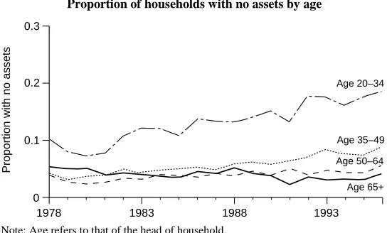
In this chapter, we present evidence from the Family Expenditure Survey on rates of ownership of different assets between 1978 and 1996. The period has seen big increases in ownership of housing, pensions and shares, but these changes have not been experienced uniformly across age and income groups. In fact, at the bottom of the wealth distribution, there are a growing number of households with no assets at all.
4.1 The Stakeholder Society
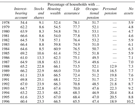
The last two decades have witnessed dramatic changes in wealth ownership in the UK. The number of households with stocks and shares and private pensions and owning their home grew enormously, particularly during the 1980s.20 However, the headline figures disguise very different experiences across age and income groups. At the bottom of the wealth distribution, there has been an increase in the number of households with no wealth at all. The broad trends in the ownership of six key asset types — interest-bearing accounts, stocks and shares, housing, life assurance, occupational pensions and personal pensions — are summarised in Table 4.1. The table shows the proportion of households in each year of the Family Expenditure Survey (FES) from 1978 to 1996 owning each of the assets and also the proportion of households with no assets at all.
TABLE 4.1
Household asset ownership
Percentage of households with …
Interest-bearing account Stocks and shares Housing wealth Life assurance Occupa-tional pension Personal pension No assets
1978 54.4 9.1 52.4 78.1 51.7 — 5.9 1979 62.2 8.6 54.5 77.7 52.1 — 4.8 1980 63.9 8.3 54.8 78.1 53.1 — 4.7 1981 66.6 8.6 54.0 77.8 53.3 — 4.6 1982 64.5 7.8 57.1 76.4 53.2 — 5.9 1983 66.4 8.8 59.8 74.9 51.0 — 6.1 1984 64.6 8.5 60.9 76.5 50.7 — 6.3 1985 69.2 10.6 61.4 75.2 51.8 — 5.9 1986 61.0 13.3 62.3 75.1 49.5 — 7.1 1987 64.9 18.8 63.1 75.4 49.6 — 7.0 1988 65.2 22.8 66.1 73.5 52.1 12.9 7.3 1989 66.2 22.9 66.0 73.0 51.8 16.5 7.7 1990 61.1 23.8 66.5 72.4 51.2 19.8 7.6 1991 69.8 25.1 68.1 72.2 51.7 21.2 7.3 1992 67.0 23.9 66.3 70.8 48.5 21.8 8.7 1993 64.7 22.8 67.4 70.0 47.6 22.3 9.2 1994 63.2 22.3 68.2 68.3 46.9 20.4 8.4 1995 61.6 23.5 67.0 68.4 47.0 20.5 8.8 1996 60.4 23.3 66.5 65.5 47.4 18.9 10.2 Note: All figures are for households with head aged 20–80.
Interest-bearing account includes Tax-Exempt Special Savings Accounts and National Savings Investment and Ordinary accounts. Ownership defined on the basis of receipt of interest income during previous 12 months.
Stocks and shares includes unit trusts, PEPs and government gilts. Ownership defined on basis of receipt of interest or dividend income during previous 12 months.
Housing includes ownership with a mortgage as well as outright ownership.
Life assurance includes fixed-term assurance, mortgage protection policies, death and burial policies, all endowment policies (including house purchase endowments) and annuities. Defined on the basis of current contributions.
Occupational pension defined on the basis of receipt of occupational pension income, for those who have already retired. For workers, defined on the basis of contributions made by the individual into an occupational pension plan, or payment of contracted-out rate of National Insurance.
Personal pension defined on the basis of individual contributions into personal pension plans, or receipt of income from personal pensions if already retired. Source: Authors’ calculations using 1978–96 FESs.
The Family Expenditure Survey (FES)
The FES has been collecting consistent data on the characteristics, expenditures and incomes of about 7,000 households every year since 1968. The data on incomes and expenditures have been used extensively in analysis of consumption growth, both over time and by different types of households (see Attanasio and Weber (1994) and Banks and Blundell (1994a), for example). The FES contains far less information on individuals’ stocks of wealth. But information on dividend income received from stocks of wealth held in interest-bearing accounts and stocks and shares and the information on contributions made to private pensions and life insurance policies can be used to construct indicator variables for whether or not households in the FES have particular assets. This is not as rich a data source as if we had information on the value of each asset, but the advantage of the FES is that the ownership variables can be constructed on a consistent basis over a long time period. This allows us to describe the main trends in patterns of ownership between 1978 and 1996, a period when ownership of many assets, such as housing, shares and pensions, was changing fairly dramatically.
number of households with life assurance. Also, at the bottom of the wealth distribution, the proportion of households with no assets at all has more than doubled since the beginning of the 1980s. In this chapter, we look in detail at what has happened to ownership of these assets across different groups of households. We examine whether the trends have been experienced uniformly across different age and income groups and we discuss some of the underlying causes of the trends.
4.2 Interest-Bearing Accounts
FIGURE 4.1
Percentage of households with an interest-bearing account
1978
Percentage of households
0 100
1993 80
60
40
20
1983 1988
Source: Authors’ calculations using 1978–96 FESs.
Figure 4.1). The series is noisy, a finding which may be attributable to the way the ownership variable is defined according to receipt of interest income and changes in the rate of interest over the period. It should be noted that other surveys have found the proportion of households with any bank or building society account to be around 90 per cent (see Kempson and Whyley (1999), Office of Fair Trading (1999) and Chapter 5), but this higher figure includes current accounts which may not pay interest.
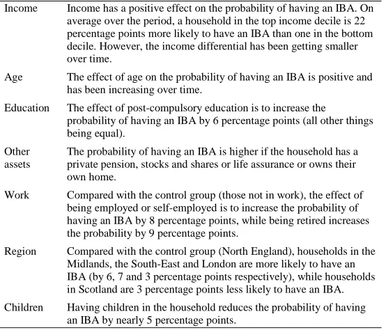
wealth or saving patterns across groups. Over time, the differential effect associated with income has been diminishing, while differences between age groups have been increasing. Although there is no significant trend in the overall proportion of households with an IBA, there is a significant downward trend in the proportion of households aged 25–34 with an IBA and a significant upward trend in the proportion of households aged 65 or over with an IBA (see Table A.2 in the appendix to this chapter).
TABLE 4.2
Ownership of interest-bearing accounts: multivariate analysis
Income Income has a positive effect on the probability of having an IBA. On average over the period, a household in the top income decile is 22 percentage points more likely to have an IBA than one in the bottom decile. However, the income differential has been getting smaller over time.
Age The effect of age on the probability of having an IBA is positive and has been increasing over time.
Education The effect of post-compulsory education is to increase the
probability of having an IBA by 6 percentage points (all other things being equal).
Other assets
The probability of having an IBA is higher if the household has a private pension, stocks and shares or life assurance or owns their own home.
Work Compared with the control group (those not in work), the effect of being employed or self-employed is to increase the probability of having an IBA by 8 percentage points, while being retired increases the probability by 9 percentage points.
Region Compared with the control group (North England), households in the Midlands, the South-East and London are more likely to have an IBA (by 6, 7 and 3 percentage points respectively), while households in Scotland are 3 percentage points less likely to have an IBA. Children Having children in the household reduces the probability of having
4.3 Stocks and Shares
At the beginning of the 1980s, fewer than one in 10 households owned shares directly. By the end of the decade, the figure was more than one in five (see Figure 4.2). Most of the increase occurred during a concentrated four-year period from 1985 to 1988, coinciding with the heavily advertised flotation of a number of public utilities, including British Telecom (1984) and British Gas (1986). Also around this time, the Conservative government introduced a further measure aimed at promoting a ‘share-owning democracy’ — namely, tax-favoured employee share schemes. Three of these — profit-sharing schemes, savings-related share option schemes and discretionary share option schemes — were introduced between 1979 and 1984.
A large part of the growth in share ownership can be directly attributed to people buying shares in the newly privatised industries. This continues to be reflected in the fact that, even by the late 1990s, a large number of
FIGURE 4.2
Percentage of households with stocks and shares
1978
Percentage of households
0 40
1993 30
20
10
1983 1988
share owners own shares only in denationalised industries (see Chapter 5). However, the evidence suggests that the growth in share ownership was not simply a one-off occurrence linked to privatisation. One reason is that the privatisation process — the extensive advertising of share flotations, for example — is likely to have promoted greater awareness of the opportunities for investing in stocks and shares more generally. Also, since the late 1980s, opportunities for investing in Personal Equity Plans (and, more recently, Individual Savings Accounts) and demutualisations of building societies are likely to have sustained the increase in share ownership among younger cohorts.
Figure 4.3 shows the level of share ownership across different date-of-birth cohorts. Without access to panel data, we cannot look at the share-ownership rates of the same individuals over time. However, by grouping together individuals in successive cross-section waves
FIGURE 4.3
Cohort profiles: share ownership
20
Proportion with shares
0 0.4
80 0.3
0.2
0.1
Age
70 60
50 40
30
1964–68
1954–58 1944–48
1934–38 1924–28 1914–18
by their date of birth, we can track average levels of share ownership among cohorts over time. Each line in Figure 4.3 represents the proportion of households of a particular date-of-birth cohort that owned shares over the period in which the cohort is observed in the FES data. For example, take the cohort born between 1944 and 1948, who enter our sample aged between 30 and 34 in 1978 (average age 32). At that time, less than 5 per cent of the cohort owned shares. We track the cohort through successive waves of the FES until 1996, when they are aged between 48 and 52 (average age 50). By this time, nearly 30 per cent of the cohort own shares.
TABLE 4.3
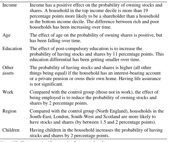
Ownership of stocks and shares: multivariate analysis
Income Income has a positive effect on the probability of owning stocks and shares. A household in the top income decile is more than 19 percentage points more likely to be a shareholder than a household in the bottom income decile. The difference between rich and poor households has been increasing over time.
Age The effect of age on the probability of owning shares is positive, but has been falling over time.
Education The effect of post-compulsory education is to increase the
probability of having stocks and shares by 11 percentage points. This education differential has been getting smaller over time.
Other assets
The probability of having stocks and shares is higher (all other things being equal) if the household has an interest-bearing account or a private pension or owns their own home. Having life assurance is not significant.
Work Compared with the control group (those not in work), the effect of being employed is to reduce the probability of owning stocks and shares by 2 percentage points.
Region Compared with the control group (North England), households in the South-East, London, South-West and Scotland are more likely to have stocks and shares (by between 1.5 and 2 percentage points). Children Having children in the household increases the probability of having
stocks and shares by 2 percentage points. Note: All effects are significant at the 5 per cent level.
older cohorts at the same age, suggesting that the increase in share ownership was more than a one-off phenomenon.
The results of a simple multivariate analysis of the relationship between household characteristics and share ownership are summarised in Table 4.3 (full results are given in the appendix to this chapter). As with interest-bearing accounts, we find that older, richer and better-educated households are more likely to own stocks and shares.
fallen from 56.5 in 1978 to 51.7 in 1996. The differential associated with higher levels of education has also fallen over time. In 1978, 63.7 per cent of households with shares had a head with post-compulsory education, compared with 33.5 per cent of all households. By 1988, the proportion of share-owning households with heads with post-compulsory education had fallen to 61.7 per cent, while the proportion of all household heads with post-compulsory education had actually increased to 41.3 per cent. However, while the differentials in share ownership between age and education groups have fallen, the multivariate analysis shows that the differential effect of income increased over the period as a whole. Towards the very end of the period, however, there was an increase in share ownership among households at the bottom of the income distribution, most likely as a result of building society demutualisations (see also Table A.3 in the appendix to this chapter).21
These findings fit the conclusions of Haliassos and Bertaut (1995) in their analysis of low levels of share ownership in the US. They attribute relatively low levels of share ownership, given the size of returns, to a lack of information. They conclude that an increase in share ownership may be brought about by extensive initial advertising plus a continuous flow of information, but that this may not be effective in drawing stockholders from lower income groups. This is an accurate portrayal of the UK experience since the early 1980s. Extensive initial advertising at the time of privatisation resulted in higher levels of share
21
ownership, which have since been sustained by PEPs, ISAs and demutualisations. Levels of share ownership grew most rapidly among younger and less well-educated households, but share owners were still predominantly drawn from those at the top of the income distribution.
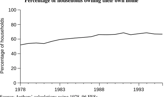
4.4 Housing
The proportion of households owning their home increased from just over half in 1978 to two-thirds in 1996 (see Figure 4.4). Most of the increase occurred during the first half of the period, coinciding with the introduction of the Conservative government’s ‘right-to-buy’ programme, which sold off council houses to their tenants, often at considerably less than market rates. In total, more than 1.6 million properties were sold as part of the right-to-buy programme.22
FIGURE 4.4
Percentage of households owning their own home
1978
Percentage of households
0 100
1993 80
60
40
20
1983 1988
Source: Authors’ calculations using 1978–96 FESs.
A second major change during this period was the liberalisation of the mortgage market. The process was begun in 1980 with the abolition of the supplementary special deposits scheme, or ‘corset’, which made it easier for banks to compete with building societies in the mortgage market.23 Competition was further opened up by a series of measures in the early 1980s aimed at deregulating the activities of building societies and, in particular, giving individual building societies control over interest rates.24 The 1980s witnessed a huge growth in mortgage lending. In 1982, the total value of mortgage loans was 32 per cent of GDP. By 1989, it was 58 per cent. There was also an increase in the average size of loans as a proportion of house prices: from 75 per cent in 1980 to 84 per cent in 1990.25
The expansion in home ownership has not been uniform across all groups of households. Figure 4.5 shows home-ownership levels across different date-of-birth cohorts. The oldest generations (those in their seventies at the end of the period) have lower levels of ownership at all ages than younger generations. People in their fifties and sixties in 1996 are much more likely to own their own homes than people in their fifties and sixties in 1978. The increase in home-ownership rates has been driven largely by this generation replacing older cohorts who were less likely to own their own homes at all ages.
However, there has not been any further increase in levels of home ownership between the middle cohorts
23
The supplementary special deposits scheme was introduced in 1973. It required banks to deposit non-interest-bearing liabilities with the Bank of England if the expansion of their interest-bearing liabilities exceeded certain rates and acted as a curb on their lending ability.
24
FIGURE 4.5
Cohort profiles: home ownership
20
Proportion owning home
0 1
80
Age
70 60
50 40
30
1944–48
1934–38
1924–28 1914–18
0.8
0.6
0.4
0.2
Note: Age is defined by the average age of the cohort each year. Source: Authors’ calculations using 1978–96 FESs.
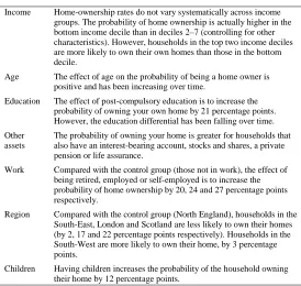
TABLE 4.4
Home ownership: multivariate analysis
Income Home-ownership rates do not vary systematically across income groups. The probability of home ownership is actually higher in the bottom income decile than in deciles 2–7 (controlling for other characteristics). However, households in the top two income deciles are more likely to own their own homes than those in the bottom decile.
Age The effect of age on the probability of being a home owner is positive and has been increasing over time.
Education The effect of post-compulsory education is to increase the probability of owning your own home by 21 percentage points. However, the education differential has been falling over time. Other
assets
The probability of owning your home is greater for households that also have an interest-bearing account, stocks and shares, a private pension or life assurance.
Work Compared with the control group (those not in work), the effect of being retired, employed or self-employed is to increase the probability of home ownership by 20, 24 and 27 percentage points respectively.
Region Compared with the control group (North England), households in the South-East, London and Scotland are less likely to own their homes (by 2, 17 and 22 percentage points respectively). Households in the South-West are more likely to own their home, by 3 percentage points.
Children Having children increases the probability of the household owning their home by 12 percentage points.
Note: All effects are significant at the 5 per cent level.
more than their current income for house purchase, while older households are typically reluctant to realise the wealth in their homes even when their incomes are low. Over time, the differential associated with age has been increasing. The biggest increase in home ownership has been among households in their fifties and sixties in 1996 (compared with households in their fifties and sixties in 1978), not among those in their twenties and thirties (see also Table A.2 in the appendix to this chapter).
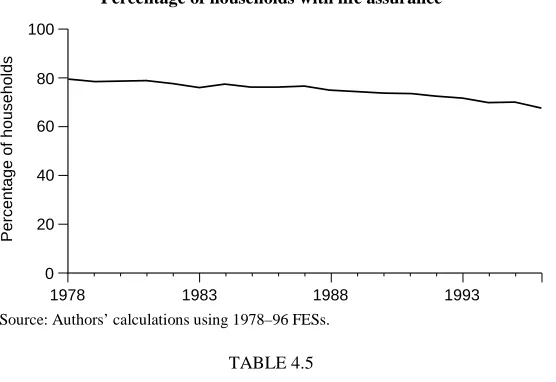
4.5 Life Assurance
Life assurance is the one asset that has seen a significant decline in ownership over the period 1978–96 (see Figure 4.6). In 1978, it was the most commonly held asset, held by nearly four out of every five households. By 1996, the proportion of households with life assurance had fallen to two-thirds. A key policy change over the period was that life assurance premiums became subject to tax from 1984. Before then, they attracted tax relief, which, since it was deducted at source, also benefited non-taxpayers.26 Clearly, the removal of tax relief is likely to have had an effect on the number of new policies taken out after 1984, although the decline in ownership had begun before then. The decline would have been greater still without a significant increase in the number of people buying homes with endowment mortgages (included in our definition of life assurance) during the 1980s. In 1991, an estimated 64.9 per cent of the premium value of new annual life policies taken out was mortgage-related.27
26
Premiums on policies taken out before 1984 continue to receive relief at the investor’s marginal tax rate.
FIGURE 4.6
Percentage of households with life assurance
1978
Percentage of households
0 100
1993 80
60
40
20
1983 1988
Source: Authors’ calculations using 1978–96 FESs.
TABLE 4.5
Life assurance: multivariate analysis
Income Households with higher incomes are more likely to have life assurance, but only up to a point. Households in the middle of the income distribution are more likely to have life assurance than those at the bottom. But households at the top of the income distribution are not much more likely to have life assurance than those in the middle.
Age The effect of age is positive and has been increasing over time. Education The effect of post-compulsory education is to reduce the probability
of having life assurance by 8 percentage points. However, this differential has been getting smaller over time.
Other assets
The probability of having life assurance is greater for households that have an interest-bearing account or a private pension or own their own home. However, households that own stocks and shares are less likely to have life assurance than those that do not. Work Compared with the control group (those not in work), the effect of
being employed, self-employed or retired is to increase the probability of having life assurance by 19, 15 and 13 percentage points respectively.
Region Compared with the control group (North England), households in the Midlands, South-East, London and South-West are less likely to have life assurance (by 4, 2, 7 and 4 percentage points respectively). Households in Scotland are more likely to have life assurance, by 6 percentage points.
Children Having children increases the probability of a household having life assurance by 8 percentage points.