HIGHLIGHTED ARTICLE GENOMIC SELECTION
Genome Properties and Prospects of Genomic
Prediction of Hybrid Performance in a Breeding
Program of Maize
Frank Technow,* Tobias A. Schrag,* Wolfgang Schipprack,* Eva Bauer,†
Henner Simianer,‡and Albrecht E. Melchinger*,1
*Institute of Plant Breeding, Seed Sciences, and Population Genetics, University of Hohenheim, 70599 Stuttgart, Germany,†Plant Breeding, Technische Universität München, 85354 Freising, Germany, and‡Department of Animal Sciences, Georg-August-University Goettingen, 37075 Goettingen, Germany
ABSTRACTMaize (Zea maysL.) serves as model plant for heterosis research and is the crop where hybrid breeding was pioneered. We analyzed genomic and phenotypic data of 1254 hybrids of a typical maize hybrid breeding program based on the important Dent3 Flint heterotic pattern. Our main objectives were to investigate genome properties of the parental lines (e.g., allele frequencies, linkage disequilibrium, and phases) and examine the prospects of genomic prediction of hybrid performance. We found high consistency of linkage phases and large differences in allele frequencies between the Dent and Flint heterotic groups in pericentromeric regions. These results can be explained by the Hill–Robertson effect and support the hypothesis of differentialfixation of alleles due to pseudo-overdominance in these regions. In pericentromeric regions we also found indications for consistent marker–QTL linkage between heterotic groups. With prediction methods GBLUP and BayesB, the cross-validation prediction accuracy ranged from 0.75 to 0.92 for grain yield and from 0.59 to 0.95 for grain moisture. The prediction accuracy of untested hybrids was highest, if both parents were parents of other hybrids in the training set, and lowest, if none of them were involved in any training set hybrid. Optimizing the composition of the training set in terms of number of lines and hybrids per line could further increase prediction accuracy. We conclude that genomic prediction facilitates a paradigm shift in hybrid breeding by focusing on the performance of experimental hybrids rather than the performance of parental lines in testcrosses.
H
YBRID breeding was pioneered in maize (Shull 1908) and plays an ever increasing role in other globally im-portant field (Duvick 1999) and vegetable crops (Silva Dias 2010). Maize has also served as a model species for research in heterosis, the phenomenon behind the success of hybrid varieties, for which the genetic mechanisms have been elusive (Duvick 1999; Lippman and Zamir 2006). In recent years, evidence emerged for the importance of (pseudo-)overdomi-nance in the manifestation of heterosis in maize (Lippmanand Zamir 2006; Schön et al. 2010) and the particular role of the centromeres in this process (Goreet al.2009; McMullen et al. 2009). Today, the availability of high-density marker data and whole-genome regression methods developed in the context of genomic prediction (Meuwissen et al. 2001) allows us to revisit this hypothesis by studying key genome properties such as allele frequencies and linkage phases.
Consistency of linkage phases between quantitative trait loci (QTL) and markers is a key prerequisite for pooling of diverse breeds and germplams to increase sample size for genetic studies and transferability of their results to different populations (De Rooset al.2008). Weberet al.(2012) used whole-genome estimates of marker effects of several cattle breeds to investigate across-breed marker–QTL linkage phase consistency. Such a study is still missing for maize and other important crops. For optimum exploitation of het-erosis, the parental inbred lines of maize hybrids are taken from genetically distant pools of germplasm, called heterotic groups (Melchinger and Gumber 1998). Comparing the Copyright © 2014 by the Genetics Society of America
doi: 10.1534/genetics.114.165860
Manuscript received March 22, 2014; accepted for publication May 19, 2014; published Early Online May 21, 2014.
Supporting information is available online athttp://www.genetics.org/lookup/suppl/ doi:10.1534/genetics.114.165860/-/DC1.
This article is dedicated to H. F. Utz on the occasion of his 75thanniversary as a
tribute to his outstanding training of generations of graduate students in selection theory at the University of Hohenheim.
1Corresponding author: Institute of Plant Breeding, Seed Sciences, and Population
profiles of marker effects of both heterotic groups would be of great interest for better understanding the genetic basis of heterosis and choice of models for genomic prediction (Technowet al.2012).
With the advent of doubled-haploid technology in many species, fully homozygous inbred lines can be generated rapidly, at low cost, and in great numbers (Wedzonyet al. 2009). This leads to a vast expansion of the number of potential hybrids. For example, with only 1000 lines gener-ated in each heterotic group every year, the number of po-tential hybrids reaches 1 million. Because producing and testing a substantial fraction of these infield trials is impos-sible, prediction of hybrid performance is of tremendous importance for hybrid breeding (Bernardo 1996).
Genomic prediction (Meuwissen et al. 2001), originally devised for prediction of breeding values, involves a“training set”of individuals that have been both genotyped and phe-notyped and a “candidate set” of untested individuals, for which only genotypic information is available (Janninket al. 2010). The genotypic values of the candidates are then pre-dicted either from their genomic relationship to the training set individuals or from marker effects estimated in the train-ing set. Genomic prediction of hybrid performance came into focus recently, with studies exploring its prospects in maize (Maenhout et al. 2010; Massmanet al. 2013), sun-flower (Reif et al. 2013), and wheat (Zhao et al. 2013). However, the low number of markers or the low number of parental lines and phenotyped hybrids used in these stud-ies allowed only preliminary inferences about the prospects of genomic prediction in commercial hybrid breeding pro-grams of ordinary size.
Optimal composition of training sets is crucial for success-ful application of genomic prediction (Rincent et al.2012; Windhausen et al. 2012). For hybrid prediction, a critical question is how many hybrids per inbred line, i.e., crosses with lines from the opposite heterotic group, should be in-cluded in the training set. With a given budget for pheno-typing of training set hybrids, the number of hybrids per line limits the total number of inbred lines that can be tested. The number of hybrids per line and the total number of lines and hybrids in the training set can affect the prediction accuracy. These important factors were not investigated in previous studies.
Technowet al.(2012) showed in a simulation study that the Bayesian whole-genome regression method BayesB (Meuwissenet al.2001) is a powerful alternative to genomic best linear unbiased prediction (GBLUP), first used by Maenhout et al. (2010) for genomic prediction of hybrid performance. Zhaoet al.(2013) later compared both meth-ods, using a wheat data set of very limited size. Thus, con-clusive results on the comparative performance of GBLUP and BayesB in real data sets are still missing.
Our objectives were to (i) investigate differences among chromosomal regions in linkage disequilibrium and linkage phases, allele frequencies, and marker effects of the parental heterotic groups; (ii) examine the prospects of genomic
prediction of hybrid performance for an important heterotic pattern in maize; (iii) investigate the effects of the size of the training set and of its composition in terms of the number of lines and the number of hybrids per line on prediction accuracy; and (iv) compare the prediction accuracy achieved by prediction methods GBLUP and BayesB. We therefore analyzed high-density genomic and phenotypic data of 1254 hybrids, collected over the last decade in a typical maize hybrid breeding program based on the Dent3Flint heterotic pattern.
Materials and Methods
Phenotypic data
Our phenotypic database comprised grain yield (GY) (in quintals per hectare) and grain moisture content (GM) (in percent) of 1254 maize single-cross hybrids generated and tested over the last decade within the breeding program of the University of Hohenheim. The hybrids represent an incomplete factorial between 123 Dent and 86 Flint inbred lines, with each Dent line involved in 10 (range 2–56) and each Flint line in 15 (range 1–102) hybrid combinations, on average. A schematic view of the factorial is shown in Sup-porting Information,Figure S1.
The data were collected in 14 years (1999–2012) and across 20 locations in Southern Germany, providing 131 envi-ronments. The field design used at each location was an a-lattice with two to three replications and incomplete block sizes offive. In total, data of 24,925field plots were available. On average, 95 hybrids, produced from 15 Dent and 11 Flint lines, were tested each year. The number of years in which a hybrid was tested ranged from 1 to 9, with an average of 1.2. Of all hybrids, 182 were tested in multiple years. The average number of years a line served as parent of one or several hybrids was 1.6 (range 1–9) for Dent lines and 1.8 for Flint lines (range 1–10).
Analysis of genomic data
All parental inbred lines were genotyped with the Illumina MaizeSNP50 BeadChip (Ganalet al.2011). We removed all markers missing or heterozygous in.5% of the inbred lines. Remaining missing (0.2%) or heterozygous (0.3%) marker genotypes were replaced with the most frequent allele. A total of 35,478 markers were subsequently available for fur-ther analysis. The marker data are provided in File S1,File S2, andFile S3.
Overall pairwise linkage disequilibrium (LD) between markers on the same chromosome was computed as r2,
Nevertheless, some density differences could not be com-pletely eliminated. This was because in some instances, no segregating markers could be found in the desired inter-vals. We then divided all chromosomes into bins of 5Mb width and computed the average pairwise LD, measured as r2, between all markers in the bin. For each bin, we also
determined the proportion of marker pairs with the same linkage phase,i.e., same sign of the rstatistic in Dent and Flint (Technow et al. 2012), and the correlation between the r values of both groups. For this, 4397 markers with a MAF$0.025 in each group were used.
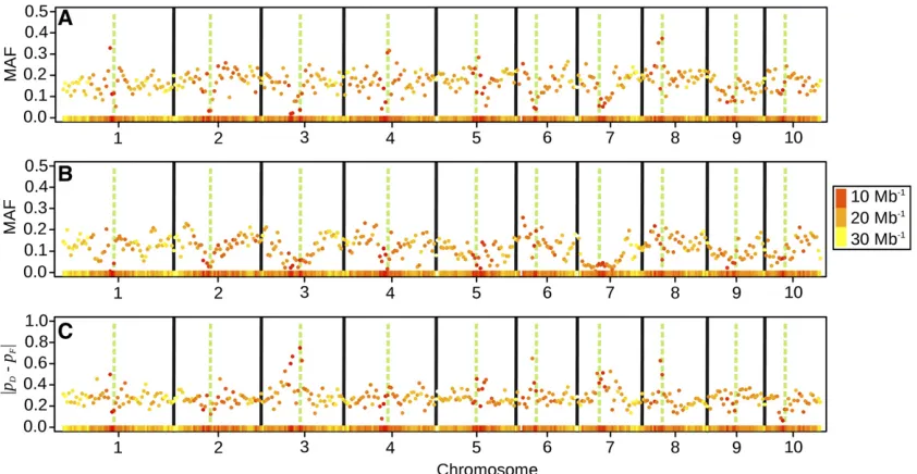
MAF patterns along the chromosomes were investigated using a similar approach. Again we used consecutive bins of 5Mb width and computed the average MAF for each bin in the sets of Dent and Flint lines as well as the average absolute difference between the reference allele frequencies in the two groups. These investigations were carried out using all 35,478 markers. The allele that had highest frequency across the combined set of Dent and Flint lines was defined as the reference allele.
Variance components and adjusted means
We used a two-stage analysis for estimation of variance components and adjusted entry means that closely followed Bernardo (1996) and Massman et al. (2013). Two-stage analysis is commonly used for analyzing plant breedingfield trials and delivers in most cases results similar to those of considerably more complex one-stage approaches (Möhring and Piepho 2009). Its main advantage is the strongly re-duced computational burden when numbers of genotypes and environments are large.
In the first stage, hybrid 3 environment means y were calculated with a standarda-lattice design analysis to adjust for the effects of the field design in these environments. In the second stage, wefitted the model
y¼XbþZDgDþZFgFþZSsþe; (1)
where vectorycontained the phenotypic observations of the hybrids in the 131 environments obtained in stage one, b was the vector offixed effects of environments, andXwas the corresponding design matrix.
The design matrices ZD and ZF associated the random
general combining ability (GCA) effects of the parental Dent lines (gD) and Flint lines (gF), respectively, to the
observa-tions of the hybrids in y. ZS was the design matrix of the
random specific combining ability (SCA) effects (s) for spe-cific Dent3 Flint hybrid combinations in y. The residuals were represented by vector e. The covariance matrix ofgD
wasGDs2D;that ofgFwasGFs2F;and that ofswasSs2s;where
s2
D;s2F;ands2s were the variance components pertaining to
GCA and SCA effects. The covariance matrix of the residuals wasRs2
R;withs 2
Rbeing the residual variance. The diagonal
elements of Rwere the reciprocals of the number of repli-cations in the environment of the corresponding data points. All other elements ofRwere zero. In the two-stage analysis
applied in our study, the genotype3environment variance cannot be separated from the residual variance associated with the adjusted means iny (Möhring and Piepho 2009). Variance components2
R therefore contained the residual as
well as the genotype3environment variance. This enabled also a direct comparison with the results of Massman et al. (2013), who used the same approach for computing vari-ance components and entry means.
The genomic relationship matrix GD was computed
according to VanRaden (2008) asGD¼WDW9D=mD;where mDffiffiffiffiffiffiffiffiffiffiffiffiffiffiffiffiffiffiffiffiffiffiffiffiffiis the number of markers and wuv¼ ðxuv22pvÞ=
4pvð12pvÞ p
(u being the index of the inbred line and v that of the marker), withxuvcoding the number of reference alleles, i.e., 0 or 2, andpvbeing the allele frequency of the reference allele in the population of Dent lines. The genomic relationship matrixGFwas computed accordingly. For
com-putingGDandGF, only markers were used that segregated
in the respective heterotic group with MAF$0.025. LetDandD* denote any two Dent lines andFandF* any two Flint lines. For a given pair of single crosses (D3F) and (D*3F*), the element ofSwas the productgDD*gFF*;where gDD*andgFF*are the corresponding elements ofGDandGF,
pertaining to D and D* and Fand F*, respectively (Stuber and Cockerham 1966).
The variance components were estimated for the whole data set, using the EM algorithm for restricted maximum likelihood described by Henderson (1985) and adapted for variance component estimation in factorials by Bernardo (1996). The entry-mean heritability was computed as H2¼ ðs2
Dþs2Fþs2sÞ=ðs2Dþs2Fþs2s þs2R=eHÞ; where eH
was the harmonic mean of the diagonal elements of Z9sR21Zs;i.e., of the total number of replications per hybrid.
Finally, environment-adjusted entry means of all hybrids (y*) were computed as y*¼ ðZ9sR21ZsÞ21Z9sR21ðy2XbÞ;
following Bernardo (1996). The adjusted entry means are provided inFile S4.
GBLUP
The performance of untested hybrids was predicted by GBLUP with the formula CUTV2TT1y*T (Henderson 1973).
Here, CUTis the genetic covariance matrix of untested and
tested hybrids, VTTis the phenotypic covariance matrix of
the tested hybrids, andy*
Tare the observed phenotypic
val-ues of the tested hybrids (a subset of y*). The elements of CUTandVTTwere computed according to Bernardo (1996),
using our estimates ofgDD* andgFF*:
BayesB
Our BayesB-type model for the performance of the ith hy-brid corresponded to model S2of Technowet al.(2012):
mi¼b0þMDiuDþMFiuFþDidDF
y*
T N
mi;s2
e
: (2)
vectors MDi;MFi; andDi are known marker genotype inci-dence vectors for the additive marker effects of the Dent parent lines inuDand Flint parent lines inuFand the
dom-inance effects in dDF. The likelihood of a single data point
was a Gaussian density with mean parameter equal to mi and variances2
e:
The elements of the matricesMDandMFcode the
pres-ence or abspres-ence of the referpres-ence allele in the gametes pro-duced by the parental Dent and Flint lines as 1/2 and21/2, respectively. In contrast to MD andMF, which code the
ge-notypes of parental gametes, matrix D directly reflects the genotypes of the single-cross hybrids, coding heterozygous genotypes as 1 and homozygous genotypes as 0. For exam-ple, if the allele contributed by the Dent parent was“C”and that by the Flint parent “T”, and T had the higher allele frequency, then the corresponding elements of MD, MF,
andDwere21/2, 1/2, and, 1, respectively.
Additive effects were estimated only for markers with a MAF$0.025 within the set of tested inbred line parents of the respective heterotic group and dominance effects only for markers with a MAF $ 0.025 in at least one of the groups. We reduced the marker density to 10 markers per megabase to facilitate computations. Using higher marker densities did not improve prediction accuracies, as far as we could see. In total, additive effects were estimated for mD= 7500 markers of the Dent parental lines and for mF= 6500 markers of Flint parental lines, on average. The
average number of markers for which dominance effects were estimated wasmDF= 8900.
Prior specifications as well as the Gibbs-sampling strategy were identical to those in Technowet al.(2012). The same uninformative prior distribution, a Gamma distribution with a=b= 0.1, was used for the scale parameterS2. However,
the hyperparametersnandpwere set to constant values, as in the original BayesB implementation of Meuwissen et al. (2001). Parameternwas set to 4.001 for all types of marker effects, andpwas chosen such that the number of markers fitted was 500, on average; e.g., for dominance effects (12pDF)mDF= 500.
Three independent Gibbs-sampling chains were run for 75,000 iterations, of which thefirst 74,000 iterations were discarded as burn-in. Using a higher number of iterations and chains did not improve prediction accuracy. The posterior means of marker effects were used to predict the performance of untested hybrids according to model (2).
For investigating the genetic architecture, namely the distribution and properties of marker effects, we fitted model (2), using all 1254 hybrids. The marker density was further reduced to 1 marker per megabase, or 1617 markers used in total. This was done mainly to counter potential problems with likelihood identifiability that can occur when the number of effects is much larger than the sample size (Gianola 2013). All markers used segregated in each set of parental inbred lines with MAF$0.025. Thus, all three types of marker effects (additive effects for Dent and Flint and dominance effects) were estimated for each
marker. For each trait, we ran 24 independent Gibbs-sampling chains for 1,000,000 iterations. We discarded thefirst 990,000 iterations as burn-in and afterward stored only samples from every 10th iteration. The posterior means of the marker effects were used as their point estimates.
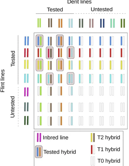
Evaluation of prediction accuracy
The cross-validation procedure for estimating prediction accuracy was stratified by the parental lines (Figure 1). LetD = {1, 2,. . ., 123} andF= {1, 2,. . ., 86} denote the entire set of Dent and Flint lines, respectively, and let the entire set of available hybrids be denoted byP= {(i,j) |i2 D, j 2 F, with hybrid combination i 3 j among the 1254 single-crosses evaluated}. As afirst step, we sampled a sub-set DT ofNDDent lines fromD and a subsetFTof NFFlint
lines from F. Then we sampled a random subsetPTof NH
training set hybrids from all hybrids for which both the Dent and Flint parents were elements ofDTandFT, respectively.
The constraint here was that for all i 2 DT and j 2 FT, nPTðiÞ$1; where nPTðiÞ is the number of hybrids i 3 j 2 PTfor theith Dent line, and likewisenPTðjÞ$1 for thejth Flint line;i.e., we made sure that all lines inDTandFTwere
parents of at least one hybrid in the training set. Hybrids in P, for which both the Dent and the Flint parents were ele-ments of DT and FT, but were not elements of PT, were
assigned to the T2 candidate group and assumed to be un-tested. All hybrids, for which the Dent parent was an ele-ment ofDTbut the Flint parent was not an element ofFTand
vice versa, were assigned to the T1 candidate group. All hybrids inP, for which neither the Dent parent nor the Flint parent was an element of DT or FT, respectively, were
assigned to the T0 candidate group.
For investigating the influence ofNH, we variedNH
be-tween 150 and 450 in steps of 50 but keptNDconstant at 90
andNFat 53. The latter restriction guaranteed that both the
required number of training set hybrids and sufficiently sized candidate groups were available for all values of NH.
The number of T2 hybrids necessarily decreased with in-creasing NH; for NH= 450, its average was still 119. The
numbers of T1 and T0 hybrids were on average 557 and 128, respectively. With increasing NH, the average number
of hybrids per Dent linecDand Flint linecFinPTincreased
fromcD¼1:69 andcF¼2:85 forNH= 150 tocD¼5:06 and cF¼8:55 forNH= 450.
For investigating the influence of the number of parental lines used in the training set, we set ND to 70 and 110,
respectively, andNFto 33 and 73, respectively, while
keep-ingNHconstant at 200. Here, the valueNH= 200 ensured
that the groups of T2, T1, and T0 hybrids had a sample size of at least 20 hybrids each for all values ofNDandNF. When ND= 70 andNF= 33, the average numbers of hybrids per
line werecD¼3:05 andcF¼6:18 (Table 3) and the average
numbers of the T2, T1, and T0 hybrids were 78, 646, and 328, respectively. When ND = 110 andNF= 73,cD¼1:82
and cF¼2:75 and the average numbers of T2, T1, and T0
The prediction accuracyrAwas computed separately for
each group of hybrids by dividing the correlation of pre-dicted and observed values (“predictive ability”) by pffiffiffiffiffiffiH2
(Legarra et al. 2008). The cross-validation process was re-peated 10,000 times for each value of NH,ND, and NF,
re-spectively. Sets DT and FT were randomly sampled each
time. Only 100 repetitions could be performed per scenario for BayesB because the computational demands of this method were considerably higher than those of GBLUP.
All analyses were carried out in the R statistical software environment (R Development Core Team 2012).
Results
Analysis of genomic data
From all 35,478 markers analyzed, 18.0% were mono-morphic in the set of Dent lines, 20.5% in the set of Flint lines, and 8.5% in both. Excluding monomorphic markers, the median MAF in the Dent pool was 0.19 and that in the Flint pool was 0.12. Marker densities were lowest in pericentromeric regions, where particularly low MAFs were found (Figure 2, A and B). The largest absolute differences between the allele frequencies in the Dent and Flint heter-otic groups were also found in pericentromeric regions (Fig-ure 2C), indicating different fixation of alleles in these regions between the two groups.
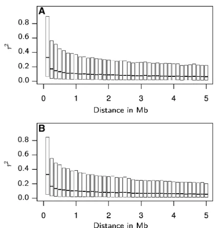
The LD in relation to physical distance reached very high median values 0.33 for markers in close proximity (,0.125 Mb), with considerable proportions of the marker pairs exhibitingr2values.0.8 (Figure 3). It then decayed to
medianr2values0.10 for marker pairs with distances of
3 Mb. The decrease in LD then continued, however, less pronounced, such that even at distances of 15 Mb, the me-dianr2was still0.05 (data not shown).
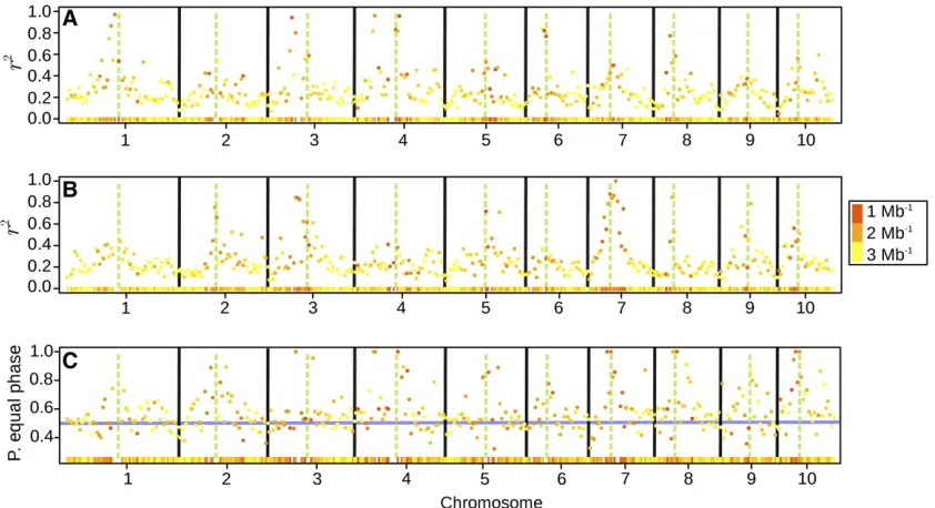
Pericentromeric regions displayed considerably elevated levels of regional LD (Figure 4, A and B). In many cases, the average pairwise r2values in pericentromeric regions were
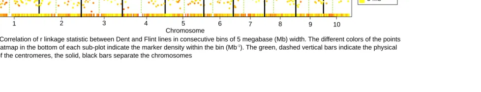
more than four times higher than those in distal chromo-some regions. Also the proportion of markers with the same sign of therlinkage statistic was higher in pericentromeric regions (Figure 4C). Here, the proportion could reach 100%, whereas in distal regions of the chromosomes it was50% (the value indicating independence of Dent and Flint link-age phases). Similar trends were observed for the regional correlation of rbetween groups, which was generally posi-tive and high in pericentromeric regions but around zero outside of these (Figure S2).
Estimated marker effects: The number of markers with
sizeable estimated additive effects was much larger than the number of markers with sizeable dominance effects (Figure S3 andFigure S4). Additive and dominance marker effect estimates were in equal proportions negative and positive. We did not observe a strong accumulation of large additive or dominance marker effects in any particular genomic re-gion or chromosome.
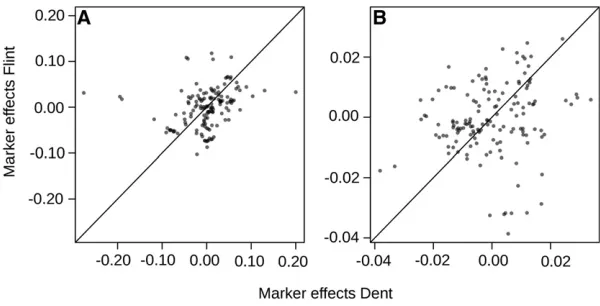
The additive marker effects estimated for Dent (uD) were
overall not consistent with those for Flint (uF). The rank
correlation between additive marker effects for Dent uD
and FlintuFwas close to zero for both traits, but when
re-stricted to markers within 12.5 Mb of the centromeres, the correlation was 0.385 (P= 0.19531025) and 0.200 (P=
0.015) for GY and GM, respectively (Figure 5).
For GY, markers with strong additive effects for both Dent and Flint were encountered in the first quarter of chromosome 1 and in the last quarters of chromosomes 4 and 7 (Figure S3). The squared correlation between the predicted genotypic values and adjusted entry means was 0.85 and 0.94 within the training set for GY and GM, respectively.
Variance components and heritabilities: For both traits,
estimates ofs2
Dands2F were of similar magnitude, withs2D
slightly larger thans2F for GY (Table 1). The variance
com-ponents2
Swas always considerably smaller than eithers 2 Dor
s2
F:The proportion of s2S in the total genetic variance was
almost twice as high for GY than for GM. Very high entry-mean heritabilities were observed for both traits.
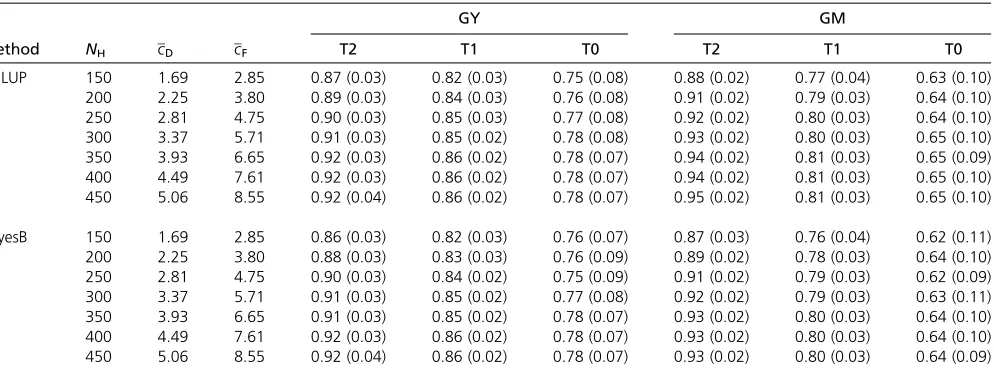
Prediction accuracies: Prediction methods GBLUP and
BayesB resulted in very similar prediction accuracies (Table 2 and Table 3). Our presentation of prediction accuracy
results therefore applies to both methods, if not mentioned otherwise.
For both traits and across all levels ofNH, the prediction
accuracy was highest for T2 hybrids, followed by T1 and T0 hybrids (Table 2). Prediction accuracies of GY were higher than those of GM for T1 and T0 hybrids but the opposite was true for T2 hybrids.
The prediction accuracyrAincreased with increasing NH
similarly for both traits (Table 2). The increase in rAwas
strongest for the T2 hybrids, followed by T1 and T0 hybrids. For example, the average increase inrAfromNH= 150 to NH= 450 was 0.06 for T2 hybrids, 0.04 for T1 hybrids, and
0.025 for T0 hybrids. For the T2 and T1 hybrids the accuracy still increased in the higher range ofNH, while for T0 hybrids
therAvalues did not increase further aboveNH= 300.
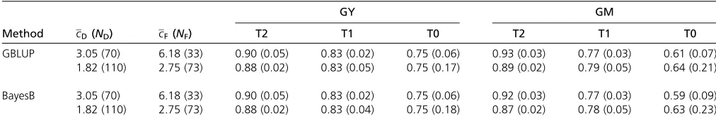
Keeping NH constant, but increasing ND and NF,
de-creased the prediction accuracy for T2 hybrids for both traits (Table 3). The difference inrAbetween the highNDandNF
scenario and the lowNDandNFscenario was 0.02 (GY) and
0.04 (GM). For GM,rAof the T1 and T0 hybrids increased
with increasingNDandNF(difference 0.03). AlteringNDand NFhad no effect onrAvalues of T0 and T1 hybrids for GY.
Discussion
Consistency of linkage phases and marker effects across heterotic groups
Establishing separate training sets of sufficient size for small breeds in animal breeding or for different germplasm groups in plant breeding is generally too expensive. In this situation, pooling data sets from several germplasm groups can increase the power of genomic selection, as demonstrated by Technow
et al.(2013) for disease resistance in maize. In cattle breed-ing, too, augmenting training sets with individuals from other breeds increased prediction accuracy to some extent (De Roos et al.2009; Hayeset al.2009; Erbeet al.2012; Weberet al. 2012).
Habier et al. (2007, 2013) showed by simulation and theory that genomic prediction methods such as GBLUP and BayesB can exploit information from pedigree relation-ships, cosegregation, and LD for prediction. Owing to the long separation of cattle breeds and heterotic groups in maize, respectively, pedigree relationships and cosegrega-tion can be ruled out as sources of informacosegrega-tion shared across groups, leaving only LD.
For major cattle breeds (De Rooset al.2008) and for the Dent and Flint heterotic groups in maize (Technow et al. 2013), linkage phases between SNP markers were indeed similar across breeds and heterotic groups, respectively. We confirmed the latter result and could further show that the consistency of linkage phases is highest in pericentromeric regions of the maize genome.
However, LD between markers is not necessarily a good indicator for LD between markers and QTL, especially when the latter have a much lower minor allele frequency than the former (Yanget al.2010). To investigate the consistency of marker–QTL LD and linkage phases across breeds, Weber et al. (2012) compared marker effect estimates of several cattle breeds, because a high similarity of marker effect pro-files across breeds would reflect consistency in marker–QTL LD. They found the similarity to be low and concluded that LD between markers and QTL did not persist across breeds. Factorial crosses between lines of two heterotic groups represent an ideal material for comparison of estimated
Figure 2(A and B) Average minor allele frequency (MAF) of SNP within consecutive bins of 5-Mb width along the chromosomes, for Dent lines (A) and Flint lines (B). (C) Average absolute difference of reference allele frequency between Dent and Flint lines in the same 5-Mb bins. The different colors of the points and the heat map in the bottom of each subplot indicate the marker density within the bin (Mb21). The green, dashed vertical bars indicate
additive marker effects of each group without confounding by different genetic backgrounds and environments. This is because each genotype of a single-cross hybrid represents a perfect combination of the two parental genomes without recombination.
In our study, additive marker effects estimated simulta-neously for Dent and Flint were generally not consistent across these groups. However, we observed that there is a considerable consistency of marker effects in pericentro-meric regions, in particular for GY. We therefore hypothe-size that the increase in prediction accuracy observed by Technowet al.(2013) when combining Dent and Flint lines in a training set was mostly attributable to the pericentro-meric regions of the genome, where linkage phases between markers and QTL are consistent across Flint and Dent. Re-gional differences in LD were also observed for cattle breeds (Sargolzaeiet al.2008). Thus, similar to maize, increases in prediction accuracy from pooled multibreed training sets might be driven by particular genomic regions with high linkage phase consistency across breeds.
An alternative approach to pooling for incorporating information from different breeds or germplasm groups was proposed by Brøndum et al. (2012). They described how genome position-specific priors for estimation of marker effects in one dairy cattle breed can be derived from marker effects estimated in a different breed. Using these genome position-specific priors increased prediction accu-racy within each breed. The method of Brøndum et al. (2012) does not require consistent linkage phase between breeds but only identical QTL positions. However, in this
way priors can be specified only for marker effect shrinkage parameters. If marker–QTL linkage phases are consistent across populations, as seems to be the case in pericentro-meric regions of maize, priors could be derived for the marker effects themselves, too. This could be achieved, for example, by changing the prior mean of the marker effect from zero to the posterior mean of the marker effect esti-mated in the other breed, population, or heterotic group.
Estimation of population-specific marker effects for genomic prediction of crossbreds and single-cross hybrids
There are many parallels between hybrid breeding in crops like maize and crossbreeding in livestock production. In simulation studies on genomic prediction with training sets consisting of crossbred individuals (Ibánez-Escriche et al. 2009; Zeng et al.2013) or single-cross hybrids (Technow et al. 2012), it was found that genomic prediction models that fitted specific marker effects for the parental popula-tions (i.e., purebred breed or heterotic group) had little or no advantage over simpler models that assumed marker effects to be the same across parental populations. One ex-planation the authors gave for this was that the linkage phase consistency across populations was sufficiently high at high marker densities. In addition, the authors argued that the strongly increased dimensionality of those models prevented them from efficiently capturing remaining across-population differences in marker effects. Knowing in which genomic regions marker–QTL linkage phases are consistent or not could also be used for developing models that esti-mate population-specific marker effects only where neces-sary. This would reduce the dimensionality of these models and might mitigate some of the problems associated with it. We also observed that fitting marker effects to be the same across heterotic groups delivered virtually the same prediction accuracy as model (2) in which specific marker effects were estimated for Dent and Flint (results not shown). This seems to contradict our observation that marker effects are consistent only in pericentromeric regions. However, as is discussed later in detail, prediction of hybrid performance is mostly driven by the presence of close relatives in the training set, in particular for T2 and T1 hybrids. As shown by Habieret al.(2007), BayesB can cap-ture such pedigree relationships, particularly when many markers are fitted. Capturing pedigree relationships with markers does not require physical linkage between them and the QTL (Habier et al.2013). Consistency of marker– QTL linkage phase might therefore not be mandatory for accurate predictions when close relatives are present in the training set.
Hill–Robertson effect and heterosis
It is known that recombination is suppressed in the pericentromeric regions of maize chromosomes (Goreet al. 2009; Schnable et al.2009; Ganalet al.2011; Baueret al. 2013) and while gene density is comparably low in these
Figure 3(A and B) Boxplots of pairwise LD, measured asr2, between
regions (Schnableet al.2009), they still contain a consider-able portion of genes (Goreet al.2009). The Hill–Robertson effect (Hill and Robertson 1966; Felsenstein 1974) describes the influence of recombination on selection efficiency. This effect predicts a buildup of repulsion-phase linkage between QTL alleles when recombination is suppressed (McVean and Charlesworth 2000). One consequence of repulsion-phase linkage is pseudo-overdominance, because additive QTL effects cancel out. Based on the Hill–Robertson effect, McMullenet al.(2009) hypothesized that the strongly sup-pressed recombination in pericentromeric regions of maize results in pseudo-overdominance and is therefore a major cause of heterosis. Larièpeet al.(2012) mapped dominance QTL in Dent3Flint crosses for important agronomic traits, using a North Carolina III design, and found a large pro-portion of QTL with (pseudo-)overdominance in pericentro-meric regions. Schön et al. (2010) observed the same for Stiff-Stalk Synthetic 3 Non-Stiff-Stalk crosses. They con-cluded that pseudo-overdominance in pericentromeric regions led to differential fixation of QTL alleles in each heterotic group. We found the largest allele frequency differ-ences between Dent and Flint in pericentromeric regions and therefore conclude that also for the Dent3Flint heter-otic pattern differential fixation in pericentromeric regions takes place.
As allele frequencies in opposite heterotic groups drift apart during reciprocal recurrent selection (Labate et al. 1999), the ratio of SCA variance to GCA variance decreases (Reif et al. 2007) and dominance effects are increasingly absorbed into the population mean or become inseparable
from additive effects (i.e., when QTL arefixed in one group but still segregate in the other). In particular, QTL with strongly positive (pseudo-)dominance or (pseudo-)over-dominance effects are expected to be affected by differential fixation. The dominance effects of these QTL increase the “baseline”heterosis of the Dent3Flint heterotic pattern but are not detectable with statistical means in our set of Dent3 Flint interpool hybrids. This can explain why dominance marker effects had positive and negative signs in almost equal proportions even though dominance effects for grain yield in maize are expected to be mostly positive (Schön et al. 2010). It also explains the absence of any noticeable accumulation of major dominance marker effect estimates in pericentromeric regions.
Comparison of prediction methods
GBLUP and BayesB achieved nearly identical prediction accuracies. Both GY and GM are considered to be highly polygenic traits, based on QTL mapping results (Schönet al. 2004; Huanget al.2010). Several authors found in simula-tion studies and for real data sets that GBLUP models were superior to or equally well performing as Bayesian whole-genome regression methods for such traits (Zhong et al. 2009; Hayes et al.2010; Clarket al.2011; Kärkkäinen and Sillanpää 2012; Technow and Melchinger 2013; Wimmer et al. 2013). Daetwyler et al. (2010) arrived at the same conclusion based on theoretical results. Zhao et al.(2013) compared several methods for genomic prediction of grain yield of wheat hybrids and also found that GBLUP delivers the same or slightly higher prediction accuracy than BayesB.
Figure 4(A and B) Average pairwise LD (measured asr2) within consecutive bins of 5-Mb width along the chromosomes, for Dent lines (A) and Flint
lines (B). (C) Proportion of marker pairs with equal linkage phase (equal sign ofrstatistic) between Dent and Flint lines in the same 5-Mb bins. The different colors of the points and the heat map in the bottom of each subplot indicate the marker density within the bin (Mb21). The green, dashed
Thus, no substantial differences between both methods are expected for prediction of hybrid performance for traits like GY and GM.
If the effects of single QTL in polygenic traits vary considerably in size, adaptively shrinking Bayesian whole-genome regression methods could potentially outperform GBLUP. Furthermore, we hypothesize that BayesB could have an advantage for prediction of performance of T0 hybrids from lines distantly related to the parents of the training set hybrids, because then prediction accuracy would mainly come from short-range LD, which is not captured optimally by GBLUP (Habieret al.2013).
Bayesian whole-genome regression methods can suffer from a lack of likelihood identifiability, when the number of markers is much larger than the size of the training set (Gianola 2013). This can lead to computational and conver-gence problems in Gibbs sampling (Gelfand and Sahu 1999). As reported by Technow and Melchinger (2013), nonidentifiability can impair prediction accuracy. Our BayesB model for prediction of hybrid performancefits up to three effects per marker, thereby exacerbating the prob-lem. Consequently, Bayesian whole-genome regression methods require larger sizes of the training set for realizing a potential advantage.
Technow et al. (2012) confirmed in a simulation study that BayesB can achieve slightly higher prediction accuracy than GBLUP under a polygenic trait architecture, with a training set comprising 800 hybrids. Assembling large training sets is possible even for moderately sized breeding programs, like the one of the University of Hohenheim. With our data set, for example, a training set of 1254 hybrids could have been assembled, albeit without the possibility of performing a thorough cross-validation. Nonetheless, given the considerably greater computational demands of Bayesian whole-genome regression methods, GBLUP seems to be a very pragmatic and robust method for genomic pre-diction of hybrid performance for polygenic traits.
Prediction accuracy of T2, T1, and T0 hybrids
We confirmed the sizeable differences in prediction accuracy between T2, T1, and T0 hybrids found in the simulation study of Technowet al.(2012). The same was observed by
Maenhoutet al.(2010) and Schraget al.(2010), who com-pared only T1 and T0 hybrids. These differences can be explained by the different numbers of parents of the hybrids that are also parents of training set hybrids (i.e., two, one, and zero for T2, T1, and T0 hybrids, respectively); the more that are shared, the higher the accuracy that can be expected (Technowet al.2012). The paramount importance of pedigree relationships relative to other potential sources of accuracy like LD between markers and QTL was convinc-ingly substantiated by Wientjeset al.(2012). In the human genetics context, De Los Camposet al.(2013) have derived an upper limit for the prediction accuracy that is a function of the accumulated relationship between individuals in the training and testing sets, respectively. The importance of close relatives for achieving highly accurate predictions was also observed in an animal breeding context (Legarra et al.2008; Habier et al.2010).
Because of the rapidly expanding arrays of genotyped lines, the number of T1 and T0 hybrids will eclipse the number of T2 hybrids. For example, if 1000 lines are available per heterotic group, of which 100 are parents of hybrids in the training set, the number of T1 hybrids reaches 180,000 and the number of T0 hybrids a staggering 810,000, while there are“only”10,000 T2 hybrids (minus those in the training set). Thus, by sheer numbers, the best hybrids are most likely found among T1 and T0 hybrids. However, owing to the lower prediction accuracies, it will be more difficult to identify them, compared to identifying superior T2 hybrids. Breeders are unlikely to rely solely on genomic predictions when selecting potential hybrids for commercialization. Rather, genomic prediction will be employed as an initial stage in a multistage selection scheme, involvingfield testing of the most promising exper-imental hybrids. The number of experexper-imental hybrids that can be tested in such a manner is limited by budget con-straints. For practical application of genomic prediction, it is therefore important to investigate how the preselection of hybrids should be informed by the different prediction ac-curacies observed in the three groups.
In an earlier study on genomic prediction of hybrid performance for GY and GM, Massman et al. (2013) also found high prediction accuracies with training set sizes
comparable to ours. The most likely explanation for the high prediction accuracies generally observed is that bothH2and
the realized relationships among parental lines tend to be very high in commercial maize breeding programs. For ex-ample, our high estimates ofH2were for both traits in close
agreement to those of Schrag et al.(2006) and Massman et al.(2013), the latter of which analyzed data from a U.S. corn-belt breeding program. Massman et al. (2013) also found similarly high pairwise realized relationships to those in our study (details not shown). For prediction of breeding values under an additive genetic model, a trait with highH2
is expected to have higherrAvalues than a trait with lowH2
(Daetwyleret al.2010). In our study, however, therAvalues
observed for GM, which had a considerably higherH2than
GY, were higher than rA for GY only for T2 hybrids, but
lower for T1 and T0 hybrids. Interestingly, Massman et al. (2013) reported exactly the samefindings, with GM having higherrAvalues than GY for T2 hybrids but lower values for
T1 hybrids (there were no T0 hybrids in their study). Re-gional differences in LD, as found in our study, are a possible explanation why the relationship between heritability and prediction accuracy differs strongly among traits (Habier et al. 2013). We hypothesize that the contribution of infor-mation from LD to the prediction accuracy differs between
T2, T1, and T0 hybrids. Regional differences in LD, there-fore, can also explain why the relationship between herita-bility and prediction accuracy is inconsistent not only among traits, but also between T2, T1, and T0 hybrids.
Composition of training set
Prediction accuracy increased with increasing training set size NH, as expected (Table 2). However, the increase was
relatively small, even when NHwas tripled. This is in
con-trast to studies on genomic prediction of additive breeding values in plant breeding, where triplingNHcould double the
accuracy (Asoro et al. 2011; Technow et al. 2013). One explanation for this is the already rather high level of pre-diction accuracy reached. On the other hand, accuracy in-creased for T2 hybrids more than for T0 hybrids, even though their prediction accuracy was already higher for smallNH.
The key point is that increasingNHfor constantNDand NFdoes not eliminate the weakness of limited sampling of
different GCA effects from each parental germplasm pool. It only increases the number of crosses cD and cF; in which
a line is tested,i.e., the number of replicates per GCA effect. Thus, the precision of estimates of GCA effects of tested lines is increased, but under a high H2, as in our study, this has
only little impact on rA. Another, more important
conse-quence of increasing the number of hybrids per line is that separation of GCA and SCA effects becomes easier, improv-ing the predictability of both. However, the contribution of SCA variance to total genetic variance was comparatively small in our data, which again limits the benefit of increas-ingNHunder constantNDandNF. Therefore, increasingNH
when ND and NF are constant, i.e., increasing cD and cF;
might have a greater impact onrAunder lowH2and in crops
or breeding programs with less defined or no heterotic
Table 1 Variance components of Dent (s2
D) and Flint (s2F) GCA
effects and SCA effects (s2
S), residual variance component (s2R),
proportion ofs2
Sin the total genetic variance in percent (% s2S),
and entry mean heritabilities (H2) for grain yield (GY) and grain
moisture content (GM)
s2
D s2F s2S s2R % s2S H2 GY (q ha21) 32.79 28.12 8.44 179.00 12.17 0.87
GM (%) 2.58 2.59 0.40 3.70 7.15 0.96
q ha21, quintals per hectare.
Table 2 Prediction accuracy (rA) of T2, T1, and T0 hybrids obtained for different numbersNHof hybrids but a constant numberND= 90 and
NF= 53 of Dent and Flint parental lines in the training set
Method NH cD cF
GY GM
T2 T1 T0 T2 T1 T0
GBLUP 150 1.69 2.85 0.87 (0.03) 0.82 (0.03) 0.75 (0.08) 0.88 (0.02) 0.77 (0.04) 0.63 (0.10) 200 2.25 3.80 0.89 (0.03) 0.84 (0.03) 0.76 (0.08) 0.91 (0.02) 0.79 (0.03) 0.64 (0.10) 250 2.81 4.75 0.90 (0.03) 0.85 (0.03) 0.77 (0.08) 0.92 (0.02) 0.80 (0.03) 0.64 (0.10) 300 3.37 5.71 0.91 (0.03) 0.85 (0.02) 0.78 (0.08) 0.93 (0.02) 0.80 (0.03) 0.65 (0.10) 350 3.93 6.65 0.92 (0.03) 0.86 (0.02) 0.78 (0.07) 0.94 (0.02) 0.81 (0.03) 0.65 (0.09) 400 4.49 7.61 0.92 (0.03) 0.86 (0.02) 0.78 (0.07) 0.94 (0.02) 0.81 (0.03) 0.65 (0.10) 450 5.06 8.55 0.92 (0.04) 0.86 (0.02) 0.78 (0.07) 0.95 (0.02) 0.81 (0.03) 0.65 (0.10)
BayesB 150 1.69 2.85 0.86 (0.03) 0.82 (0.03) 0.76 (0.07) 0.87 (0.03) 0.76 (0.04) 0.62 (0.11) 200 2.25 3.80 0.88 (0.03) 0.83 (0.03) 0.76 (0.09) 0.89 (0.02) 0.78 (0.03) 0.64 (0.10) 250 2.81 4.75 0.90 (0.03) 0.84 (0.02) 0.75 (0.09) 0.91 (0.02) 0.79 (0.03) 0.62 (0.09) 300 3.37 5.71 0.91 (0.03) 0.85 (0.02) 0.77 (0.08) 0.92 (0.02) 0.79 (0.03) 0.63 (0.11) 350 3.93 6.65 0.91 (0.03) 0.85 (0.02) 0.78 (0.07) 0.93 (0.02) 0.80 (0.03) 0.64 (0.10) 400 4.49 7.61 0.92 (0.03) 0.86 (0.02) 0.78 (0.07) 0.93 (0.02) 0.80 (0.03) 0.64 (0.10) 450 5.06 8.55 0.92 (0.04) 0.86 (0.02) 0.78 (0.07) 0.93 (0.02) 0.80 (0.03) 0.64 (0.09)
cDandcFrefer to the average number of hybrid combinations in the training setPTfor the Dent and Flint lines in the training set. The values refer to the mean (standard
groups, where the relative contribution of SCA variance is expected to be larger (Reifet al.2007).
Nonetheless, increasing the number of hybridscDandcFfor
lines serving as parents of hybrids in the training set will in-crease the prediction accuracy for GCA effects of these lines, which is especially beneficial under low contribution of SCA variance, because then the performance of a hybrid can be approximated by the sum of the parental GCA effects. This explains why prediction accuracy of untested hybrids profits most from increasingNHif both parents were parents of other
hybrids in the training set (T2 hybrids) and least if none of them were involved in any training set hybrid (T0 hybrids). As expected under this rationale, therAincrease for T1 hybrids,
of which only one parental line is a parent of hybrids in the training set, was between that of the T2 and T0 hybrids.
Increasing the number of tested lines ND and NFwhile
keeping NHconstant decreased the number of hybrids per
linecD andcF in the same manner as decreasing NHwhile
keepingNDandNFconstant. The same reasoning therefore
applies here, which explains why the prediction accuracy of T2 hybrids decreased when ND and NFwere increased. In
contrast to the scenario of constantNDandNFand varying NH, the decrease in cD and cF did not lead to decreasing
prediction accuracy for GY of T1 and T0 hybrids and for GM, therAvalues even increased. The reason is that
increas-ingNDandNFnot only decreasedcD andcF but also at the
same time widened the array of germplasm covered in the training set. Thus, untested parent lines of T1 and T0 hybrids are represented better, which improved prediction accuracy of their GCA effects. Not all allele combinations encountered in T1 and T0 hybrids are present in narrow training sets and, consequently, their effects are not predict-able. More diverse and larger training sets, therefore, might also improve predictability of SCA effects.
An increase of 40 lines and a 34% and 53% decrease incD
and cF; respectively, between the high and lowND and NF
scenarios might have been too small to observe major effects. Further research is warranted to design the training set in an optimum manner so that the prediction accuracies of T2, T1, and T0 hybrids are balanced in a way that achieves maximum selection gain across all three groups. In the short term, this is possible only with simulations, because the resources re-quired for phenotyping larger factorials are prohibitive.
Habieret al.(2010) studied the role of pedigree relation-ships on accuracy of genomic prediction in German Holstein cattle. They found that prediction accuracy decreased only slightly when the training set size was halved as long as the number of close relatives per validation set individual remained constant. In a study on genomic prediction in maize, Albrechtet al.(2011) also observed that the drop in prediction accuracy was small when the training set size was halved. This was most likely a consequence of the presence of close relatives, too, because in their cross-validation scheme, an individual in the validation set had in most cases several full sibs in the training set. These studies demonstrate the disproportional importance of the closest relatives for predic-tion accuracy. Per definition, hybrids from the T2 and T1 groups always have very close relatives in the training set that share 50% of their genome. However, for hybrids from the T0 group, too, the maximum genomic relationships (i.e., estimated from marker data) to hybrids in the training set remained virtually unchanged by varying NH orND andNF
(results not shown). This is a consequence of the high degree of relationship between the inbred lines in a closed, medium-sized breeding program. The rather small differences in pre-diction accuracy between the various scenarios investigated reflect the presence of close relatives that determined predic-tion accuracy. A comparison of the predicpredic-tion accuracies of our genomic methods with those of pedigree-based methods (Bernardo 1996) could be used to quantify the contribution of pedigree relationships to the prediction accuracy. However, different from the situation in animal breeding, pedigrees of our lines were often incomplete and rarely extended more than two generations. A simulation study, in which pedigree relationships are known without error and maximum rela-tionships can be varied, might help to clarify the role that close relatives have in determining the accuracy with which hybrid performance can be predicted.
Estimates ofrAshowed a larger variation for the T0 group
compared to the T2 and T1 groups. The lower variability for the T1 and T2 groups can be explained by the guaranteed presence of close relatives in the training set. The maximum relationship of T0 group hybrids with hybrids in the training set fluctuates between replications (even though it is high and similar between scenarios, on average). However, tech-nical limitations, such as sampling constraints and different
Table 3 Prediction accuracy (rA) of T2, T1, and T0 hybrids obtained for different numbers of Dent (ND) and Flint (NF) parental lines in the
training setPTand average number of hybrid combinations per Dent line (cD) and Flint line (cF) inPT
Method cD(ND) cF(NF)
GY GM
T2 T1 T0 T2 T1 T0
GBLUP 3.05 (70) 6.18 (33) 0.90 (0.05) 0.83 (0.02) 0.75 (0.06) 0.93 (0.03) 0.77 (0.03) 0.61 (0.07) 1.82 (110) 2.75 (73) 0.88 (0.02) 0.83 (0.05) 0.75 (0.17) 0.89 (0.02) 0.79 (0.05) 0.64 (0.21)
BayesB 3.05 (70) 6.18 (33) 0.90 (0.05) 0.83 (0.02) 0.75 (0.06) 0.92 (0.03) 0.77 (0.03) 0.59 (0.09) 1.82 (110) 2.75 (73) 0.88 (0.02) 0.83 (0.04) 0.75 (0.18) 0.87 (0.02) 0.78 (0.05) 0.63 (0.23)
The size of the training set was held constant atNH= 200. The values refer to the mean (standard deviation) over 10,000 and 100 cross-validation runs with the prediction
sizes of validation groups, most likely also contributed to the observed differences.
Back to the basics: a paradigm shift
Shull (1908), the inventor of hybrid breeding, recognized that afield (i.e., population) of maize is a mixture of many unique hybrids. Based on this, he defined the tasks of a maize breeder as (a) identifying the best hybrid and (b) reproduc-ing it on a large scale. However, the classical approach of hybrid breeding with recurrent selfing has put great weight on the identification of inbred line parents with superiorper se and testcross performance. Testing of experimental hybrids was carried out only in the very last stage of each breeding cycle, when the genetic variability was already largely exhausted. Genomic prediction of hybrid perfor-mance allows focusing on single-cross hybrids from the very beginning. At the same time, doubled-haploid technology and high-throughput genotyping facilitate direct capturing and genetic characterization of vast arrays of lines from each heterotic group. Together, these technologies enable a para-digm shift in hybrid breeding and direct implementation of Shull’s groundbreaking ideas for thefirst time.
Acknowledgments
We acknowledge the excellent technical assistance of the staff members of the maize breeding program of the University of Hohenheim, especially Dietrich Klein, in conducting part of the field trials for this study. We are indebted to the group of Ruedi Fries, from Technische Universität München, for the SNP genotyping of the paren-tal lines. We also thank the three anonymous reviewers of the initial version of the manuscript for their very helpful input and suggestions. This research was funded by the Ger-man Federal Ministry of Education and Research within the AgroClustEr “Synbreed—Synergistic plant and animal breeding”(FKZ:0315528d).
Literature Cited
Albrecht, T., V. Wimmer, H.-J. Auinger, M. Erbe, C. Knaak et al., 2011 Genome-based prediction of testcross values in maize. Theor. Appl. Genet. 123: 339–350.
Asoro, F. G., M. A. Newell, W. D. Beavis, M. P. Scott, and J.-L. Jannink, 2011 Accuracy and training population design for genomic selection on quantitative traits in elite North American oats. Plant Genome 4: 132–144.
Bauer, E., M. Falque, H. Walter, C. Bauland, C. Camisan et al., 2013 Intraspecific variation of recombination rate in maize. Genome Biol. 14: R103.
Bernardo, R., 1996 Best linear unbiased prediction of maize single-cross performance. Crop Sci. 36: 50–56.
Brøndum, R. F., G. Su, M. S. Lund, P. J. Bowman, M. E. Goddard
et al., 2012 Genome position specific priors for genomic
pre-diction. BMC Genomics 13: 543.
Clark, S., J. M. Hickey, and J. H. van der Werf, 2011 Different models of genetic variation and their effect on genomic evalua-tion. Genet. Sel. Evol. 43: 18.
Daetwyler, H. D., R. Pong-Wong, B. Villanueva, and J. A. Woolliams, 2010 The impact of genetic architecture on genome-wide eval-uation methods. Genetics 185: 1021–1031.
de Los Campos, G., A. I. Vazquez, R. Fernando, Y. C. Klimentidis, and D. Sorensen, 2013 Prediction of complex human traits using the genomic best linear unbiased predictor. PLoS Genet. 9: e1003608.
de Roos, A. P. W., B. J. Hayes, R. J. Spelman, and M. E. Goddard, 2008 Linkage disequilibrium and persistence of phase in Holstein-Friesian, Jersey and Angus cattle. Genetics 179: 1503–1512. de Roos, A. P. W., B. J. Hayes, and M. E. Goddard, 2009 Reliability of genomic predictions across multiple popu-lations. Genetics 183: 1545–1553.
Duvick, D., 1999 Heterosis: feeding people and protecting natural resources, pp. 19–29 inThe Genetics and Exploitation of Heterosis
in Crops, edited by J. Coors, and S. Pandey. CSSA, Madison, WI.
Erbe, M., B. J. Hayes, L. K. Matukumalli, S. Goswami, P. J. Bowman
et al., 2012 Improving accuracy of genomic predictions within
and between dairy cattle breeds with imputed high-density sin-gle nucleotide polymorphism panels. J. Dairy Sci. 95: 4114– 4129.
Felsenstein, J., 1974 The evolutionary advantage of recombina-tion. Genetics 78: 737–756.
Ganal, M. W., G. Durstewitz, A. Polley, A. Bérard, E. S. Buckler
et al., 2011 A large maize (Zea mays L.) SNP genotyping
ar-ray: development and germplasm genotyping, and genetic map-ping to compare with the B73 reference genome. PLoS ONE 6: e28334.
Gelfand, A. E., and S. K. Sahu, 1999 Identifiability, improper pri-ors and Gibbs sampling for generalized linear models. J. Am. Stat. Assoc. 94: 247–253.
Gianola, D., 2013 Priors in whole-genome regression: the Bayes-ian alphabet returns. Genetics 194: 573–596.
Gore, M. A., J.-M. Chia, R. J. Elshire, Q. Sun, E. S. Ersoz et al., 2009 A first-generation haplotype map of maize. Science 326: 1115–1117.
Habier, D., R. L. Fernando, and J. C. M. Dekkers, 2007 The impact of genetic relationship information on genome-assisted breeding values. Genetics 177: 2389–2397.
Habier, D., J. Tetens, F.-R. Seefried, P. Lichtner, and G. Thaller, 2010 The impact of genetic relationship information on geno-mic breeding values in German Holstein cattle. Genet. Sel. Evol. 42: 5.
Habier, D., R. L. Fernando, and D. J. Garrick, 2013 Genomic-BLUP decoded: a look into the black box of genomic prediction. Ge-netics 194: 597–607.
Hayes, B. J., P. J. Bowman, A. C. Chamberlain, K. Verbyla, and M. E. Goddard, 2009 Accuracy of genomic breeding values in multi-breed dairy cattle populations. Genet. Sel. Evol. 41: 51. Hayes, B. J., J. Pryce, A. J. Chamberlain, P. J. Bowman, and M.
Goddard, 2010 Genetic architecture of complex traits and ac-curacy of genomic prediction: coat colour, milk-fat percentage, and type in Holstein cattle as contrasting model traits. PLoS Genet. 6: e1001139.
Henderson, C., 1973 Sire evaluation and genetic trends. J. Anim. Sci. 1973: 10–41.
Henderson, C., 1985 Best linear unbiased prediction of nonadditive genetic merits in noninbred populations. J. Anim. Sci. 60: 111–117. Hill, W. G., and A. Robertson, 1966 The effect of linkage on limits
to artificial selection. Genet. Res. 8: 269–294.
Huang, Y.-F., D. Madur, V. Combes, C. L. Ky, D. Coubriche et al., 2010 The genetic architecture of grain yield and related traits in Zea maize L. revealed by comparing intermated and conven-tional populations. Genetics 186: 395–404.
Jannink, J.-L., A. J. Lorenz, and H. Iwata, 2010 Genomic selection in plant breeding: from theory to practice. Brief. Funct. Ge-nomics Proteomics 9: 166–177.
Kärkkäinen, H. P., and M. J. Sillanpää, 2012 Back to basics for Bayesian model building in genomic selection. Genetics 191: 969–987.
Labate, J., K. Lamkey, M. Lee, and W. Woodman, 1999 Temporal changes in allele frequencies in two reciprocally selected maize populations. Theor. Appl. Genet. 99: 1166–1178.
Larièpe, A, B Mangin, S Jasson, V Combes, and F Dumas et al., 2012 The genetic basis of heterosis: multiparental quantitative trait loci mapping reveals contrasted levels of apparent over-dominance among traits of agronomical interest in maize (Zea maysL.). Genetics 190: 795–811.
Legarra, A., C. Robert-Granié, E. Manfredi, and J.-M. Elsen, 2008 Performance of genomic selection in mice. Genetics 180: 611–618.
Lippman, Z. B., and D. Zamir, 2006 Heterosis: revisiting the magic. Trends Genet. 23: 60–66.
Maenhout, S., B. De Baets, and G. Haesaert, 2010 Prediction of maize single-cross hybrid performance: support vector machine regression vs.best linear prediction. Theor. Appl. Genet. 120: 415–427.
Massman, J. M., A. Gordillo, R. E. Lorenzana, and R. Bernardo, 2013 Genomewide predictions from maize single-cross data. Theor. Appl. Genet. 126: 13–22.
McMullen, M. D., S. Kresovich, H. S. Villeda, P. Bradbury, H. Li
et al., 2009 Genetic properties of the maize nested association
mapping population. Science 325: 737–740.
McVean, G. A., and B. Charlesworth, 2000 The effects of Hill-Robertson interference between weakly selected mutations on patterns of molecular evolution and variation. Genetics 155: 929–944.
Melchinger, A. E., and R. K. Gumber, 1998 Overview of heterosis and heterotic groups in agronomic crops, pp. 29–44 inConcepts
and Breeding of Heterosis in Crop Plants, edited by K. R. Lamkey,
and J. E. Staub. CSSA, Madison, WI.
Meuwissen, T. H. E., B. J. Hayes, and M. E. Goddard, 2001 Prediction of total genetic value using genome-wide dense marker maps. Genetics 157: 1819–1829.
Möhring, J., and H.-P. Piepho, 2009 Comparison of weighting in two-stage analysis of plant breeding trials. Crop Sci. 49: 1977– 1988.
R Development Core Team, 2012 R: A Language and Environment
for Statistical Computing. R Development Core Team, Vienna.
Reif, J. C., F.-M. Gumpert, S. Fischer, and A. E. Melchinger, 2007 Impact of interpopulation divergence on additive and dominance variance in hybrid populations. Genetics 176: 1931–1934.
Reif, J. C., Y. Zhao, T. Würschum, M. Gowda, and V. Hahn, 2013 Genomic prediction of sunflower hybrid performance. Plant Breed. 132: 107–114.
Rincent, R., D. Laloe, S. Nicolas, T. Altmann, D. Brunel et al., 2012 Maximizing the reliability of genomic selection by optimiz-ing the calibration set of reference individuals: comparison of meth-ods in two diverse groups of maize. Genetics 192: 715–728. Sargolzaei, M., F. S. Schenkel, G. B. Jansen, and L. R. Schaeffer,
2008 Extent of linkage disequilibrium in Holstein cattle in North America. J. Dairy Sci. 91: 2106–2117.
Schnable, P. S., D. Ware, R. S. Fulton, J. C. Stein, and F. Wei, 2009 The B73 maize genome: complexity, diversity, and dy-namics. Science 326: 1112–1115.
Schön, C. C., H. F. Utz, S. Groh, B. Truberg, S. Openshaw et al., 2004 Quantitative trait locus mapping based on resampling in a vast maize testcross experiment and its relevance to quantita-tive genetics for complex traits. Genetics 167: 485–498.
Schön, C. C., B. S. Dhillon, H. F. Utz, and A. E. Melchinger, 2010 High congruency of QTL positions for heterosis of grain yield in three crosses of maize. Theor. Appl. Genet. 120: 321– 332.
Schrag, T. A., A. E. Melchinger, A. P. Sørensen, and M. Frisch, 2006 Prediction of single-cross hybrid performance for grain yield and grain dry matter content in maize using AFLP markers associated with QTL. Theor. Appl. Genet. 113: 1037–1047. Schrag, T. A., J. Möhring, A. E. Melchinger, B. Kusterer, B. S. Dhillon
et al., 2010 Prediction of hybrid performance in maize using
molecular markers and joint analyses of hybrids and parental inbreds. Theor. Appl. Genet. 120: 451–461.
Shull, G. H., 1908 The composition of afield of maize. J. Hered. os-4: 296–301.
Silva Dias, J. C., 2010 Impact of improved vegetable cultivars in overcoming food insecurity. Euphytica 176: 125–136.
Stuber, C., and C. Cockerham, 1966 Gene effects and variances in hybrid populations. Genetics 54: 1279–1286.
Technow, F., and A. E. Melchinger, 2013 Genomic prediction of dichotomous traits with Bayesian logistic models. Theor. Appl. Genet. 126: 1133–1143.
Technow, F., C. Riedelsheimer, T. A. Schrag, and A. E. Melchinger, 2012 Genomic prediction of hybrid performance in maize with models incorporating dominance and population specific marker effects. Theor. Appl. Genet. 125: 1181–1194.
Technow, F., A. Bürger, and A. E. Melchinger, 2013 Genomic pre-diction of northern corn leaf blight resistance in maize with combined or separated training sets for heterotic groups. G3 3: 197–203.
VanRaden, P. M., 2008 Efficient methods to compute genomic predictions. J. Dairy Sci. 91: 4414–4423.
Weber, K. L., R. M. Thallman, J. W. Keele, W. M. Snelling, G. L. Bennettet al., 2012 Accuracy of genomic breeding values in multibreed beef cattle populations derived from deregressed breeding values and phenotypes. J. Anim. Sci. 90: 4177–4190. Wedzony, M., B. Forster, I. Zur, E. Golemiec, M. Szechynska-Hebda
et al., 2009 Progress in doubled haploid technology in higher
plants, pp. 1–33 in Advances in Haploid Production in Higher
Plants, edited by A. Touraev, B. Forster, and S. Jain.
Springer-Verlag, Dordrecht, The Netherlands.
Wientjes, Y. C. J., R. F. Veerkamp, and M. P. L. Calus, 2012 The effect of linkage disequilibrium and family relationships on the reliability of genomic prediction. Genetics 193: 621–631. Wimmer, V., C. Lehermeier, T. Albrecht, H.-J. Auinger, Y. Wang
et al., 2013 Genome-wide prediction of traits with different
genetic architecture through efficient variable selection. Genet-ics 195: 573–587.
Windhausen, V. S., G. N. Atlin, J. M. Hickey, J. Crossa, J.-L. Jannink
et al., 2012 Effectiveness of genomic prediction of maize
hy-brid performance in different breeding populations and environ-ments. G3 2: 1427–1436.
Yang, J., B. Benyamin, B. P. McEvoy, S. Gordon, A. K. Henderset al., 2010 Common SNPs explain a large proportion of the herita-bility for human height. Nat. Genet. 42: 565–569.
Zeng, J., A. Toosi, R. L. Fernando, J. C. M. Dekkers, and D. J. Garrick, 2013 Genomic selection of purebred animals for crossbred performance in the presence of dominant gene action. Genet. Sel. Evol. 45: 11.
Zhao, Y., J. Zeng, R. Fernando, and J. C. Reif, 2013 Genomic prediction of hybrid wheat performance. Crop Sci. 53: 802–810. Zhong, S., J. C. M. Dekkers, R. L. Fernando, and J.-L. Jannink, 2009 Factors affecting accuracy from genomic selection in populations derived from multiple inbred lines: a barley case study. Genetics 182: 355–364.
GENETICS
Supporting Information
http://www.genetics.org/lookup/suppl/doi:10.1534/genetics.114.165860/-/DC1
Genome Properties and Prospects of Genomic
Prediction of Hybrid Performance in a Breeding
Program of Maize
Frank Technow, Tobias A. Schrag, Wolfgang Schipprack, Eva Bauer, Henner Simianer, and Albrecht E. Melchinger
Figure S1 Schematic illustration of factorial. Schematic view of factorial of 123 Dent and 86 Flint lines for illustration purposes. The lines appear in approximately chronological order. Produced and tested hybrids are indicated by orange squares.
1 1 1 1 1 1 1
1 1 1 1
1 1 3 1 1 2 1 1 1 1 1
1 1 2 1 1 1
2 1 1 3 2 1 1 1 2 1 1 1
1 1 1
1 1 1
1 1 1 1
1 2 1 2 1 1 1 1 1
1 1 1 1
1 1 1 1
1 2 3 1 2 2 1 9 1 1 5 1 4 1 1 1 1 1 1 1 4 1 1 1 2 1 1 1 1 1 1 1 3 1 2 1 3 1 1 1 2 1 1 1 1 2 1 1 1 1 1 1 1 1
1 1 1 1
1 1 1 1
1 1 1 1
1 1 1 1 1 1 1 1 1 1 1 1 1 1 1 1 1 1 1 1 1
1 2 1 2 1 2 1 1 1 1 1 1 1 1 1 1 1 1 1 1 1 1 1 1
1 2 1 2 2 2 1 1 1 1 1 1 1 1 1 1 1 1 1 1 1 1 1 1
1 1 1 1 1 1 1 1 1 1 1 1 1 1 1 1 1 1 1 1 1
1 1 1 1 1 1
1 1 1 1 1 1 1
1 1 1 1 1 1
1 1 1 1 1 1
1 1 1 1 1 1
2 1 1 5 5 2 1 1 1 1 1 1 1 2 1 1 1 1 2 1 1 1 1 1 2 1
1 1 1 1 1 1
1 1 1 1 1 1
1 1 1 1 1 1
1 1 1 1 1 1
1 1 1 1 1 1
1 1 1 1 1 1 1 1 1 1 1 1 1
1 1 1 1
1 1 1 1
1 1 1 1
2 2 2 1 1 1 1 1 1 1 1 1 1 1 1 1
2 6 3 1 3 1 1 1 3 1 1 3 2 4 1 2 3 1 2 1 1 1 1 1 2 1 1 1 1 1 1 1 1 1 1 1 1 1 1
1 1 1
2 2 1 1 1 1
1 3 3 2 1 1 1 1 1 1 1 2 2 1 1
2 2 1 1 1
1 1 1 1 1 1 1 1 1
1 1 1 1 1 1 1 1 1 1 1 1 1 1 1 1 1 1
2 2 1 1 1 1
1 1 1
1 1
1 4 2 1 1 1 1 1 1 1 1 1
1 1 1 1
1 1 1 1 1 1 1 1 1 1 1
1 1 1 1 1 1 1 1 1 1 1
1 3 2 1 1 1 1 1 1 1
1 1 1 1
1 1 1 1
1 2 1 1 2 1 1 1 1
1 1 1 1
1 1 1 1
1 1 1 1
1 1 1 1
1 2 1 1 1 1 1 2 1 1 1 1 1
1 2 1 1 1 1 1
1 3 2 1 1 2 1 1 1 2 1 1 1 1 1 1 1 1
1 3 4 1 1 2 3 2 1 3 1 1 1 3 1 1 1 1 1 1 1 1 1 1 1 1 1
1 2 2 1 1 2 1 1 1 1 1 1 1 1 1 1
1 1 1 1
1 1 1 1
1 1 1 1
1 1 1 1
1 1 1 1
2 1 1 1 1 1 1 1 2 1 1 1 1 1 1 1 1
1 1 1 1
1 1 1 1
2 2 1 1 2 1 2 1 2 1 1 1 2 1 1 1 1 1 1 1 1 1 1 1
1 1 1 1
1 1 1 1
1 1 1 1 1 1 1 1 1 1 1 1 1 1 1
1 1 1 1 1 1 1 1 1 1 1 1 1 1 1
1 1 1 1 1 1 1 1 1 1 1 1 1 1 1
1 1 1 1 1 1 1 1 1 1 1 1 1 1 1
1 1 1 1
2 2 1 1 1 2 1 1 1 1 1
2 2 2 1 1 1 2 1 1 1 1 1 1 1 1
1 1 1 1 1 1 1 1 1 1 1
1 1 1 1 1 1 1
1 1 1 1 1 1 1
1 1 1 1 1 1 1 1 1 1 1
1 1 1 1 1 1 1
2 1 1 1 2 1 2 2 1 1 1 2 1 1 1 1 1 1
1 1 1 1 1 1 1 1 1 1 1
1 1 1 1
1 1 1 1 1 1 1 1 1 1 1
Flint lines
De
nt
lin
Figure S2
Regional correlation ofrlinkage statistic
1 Mb-1
1 2 3 4 5 6 7 8 9 10
0.0 0.5 1.0
2 Mb-1
3 Mb-1
Chromosome
Figure S2 Correlation of r linkage statistic between Dent and Flint lines in consecutive bins of 5 megabase (Mb) width. The different colors of the points and the heatmap in the bottom of each sub-plot indicate the marker density within the bin (Mb-1). The green, dashed vertical bars indicate the physical
1 2 3 4 5 6 7 8 9 10
1 2 3 4 5 6 7 8 9 10
1 2 3 4 5 6 7 8 9 10
-1.5 -1.0 -0.5 0.0 0.5 1.0
-1.5 -1.0 -0.5 0.0 0.5 1.0
-1.5 -1.0 -0.5 0.0 0.5 1.0
-1.5 -1.0 -0.5 0.0 0.5 1.0
A
B
C
Chromosome
Figure S3 Marker effect estimates for grain yield.Posterior means of marker effect estimates for grain yield
obtained by BayesB, using a subset of 1617 markers, and all 1254 hybrids. (A) additive marker effects for Dent,
(B) additive marker effects for Flint, (C) dominance marker effects. The green, dashed vertical bars indicate the
Chromosome
-0.2 0.0 0.2 0.4 0.6 0.8
1 2 3 4 5 6 7 8 9 10
1 2 3 4 5 6 7 8 9 10
1 2 3 4 5 6 7 8 9 10 -0.2
0.0 0.2 0.4 0.6 0.8
-0.2 0.0 0.2 0.4 0.6 0.8
A
B
C
Figure S4 Marker effect estimates for grain moisture.Posterior means of marker effect estimates for grain
moisture obtained by BayesB, using a subset of 1617 markers, and all 1254 hybrids. (A) additive marker effects
for Dent, (B) additive marker effects for Flint, (C) dominance marker effects. The green, dashed vertical bars
Files S1‐S4
Available for download as .csv files at http://www.genetics.org/lookup/suppl/doi:10.1534/genetics.114.165860/‐/DC1
File S1 Marker genotypes of Dent lines
File S2 Marker genotypes of Flint lines
File S3 Map of marker data