WILKINS, JAMES K. The Influence of Classical and Non-Classical Friction on Sliding. (Under the direction of Dr. Vernon Matzen).
This study has identified two types of friction, referred to as non-classical, that are found when dealing with vinyl flooring tiles that are not well represented by the classical definition. One type of non-classical friction has a coefficient of static friction, µs, which increases the longer the body is at rest relative to its base. The other type of friction has a kinetic coefficient of friction, µk, which increases the faster the unanchored body is moving relative to its base. Techniques were developed to quantify these behaviors so they could be modeled accurately for seismic analysis. The experimental reconciliation between the predicted and the measured displacement time-histories were very good for both varieties of non-classical friction and were generally less than 10% different under uniaxial seismic accelerations. For the velocity dependent variety of friction, biaxial test results which incorporate vertical acceleration were also good.
Using these test results, analytical studies were conducted to derive a procedure which could possibly be used for the sliding analysis of unanchored objects. Several
slip. Using hazard curves from several sites and fragility curves developed from this
earthquake population, probability of failure charts were generated and comparisons between classical and non-classical friction were conducted. It was observed that non-classical systems consistently have a lower probability of failure than classical systems. The
i
The Influence of Classical and Non-Classical Friction on Sliding
by
James Kevin Wilkins
A dissertation submitted to the Graduate Faculty of North Carolina State University
In partial fulfillment of the Requirements for the Degree of
Doctor of Philosophy
Civil Engineering
Raleigh, North Carolina 2009
APPROVED BY:
Dr. Dick Keltie Dr. C.C. Tung
Dr. Vernon Matzen Dr. Abhinav Gupta
ii
BIOGRAPHY
The author was born in Henderson North Carolina on May 29th, 1970. He was raised in Garner, North Carolina and graduated from Garner Senior High School in 1988. He attended North Carolina State University until the fall of 1992 and graduated with a Bachelor of Science degree in geology. He worked for the North Carolina Department of Transportation with the Geotechnical Unit until returning to North Carolina State University full time in 1999. While taking civil engineering classes, he found that he enjoyed working with
iii
ACKNOWLEDGEMENTS
iv
LIST OF TABLES vi
LIST OF FIGURES viii
CHAPTER 1 Introduction 1
1.1 General Introduction 1
1.2 Background 4
1.3 Literature Review 7
1.4 Research Objectives and Organization of this Study 19 CHAPTER 2 Non-Classical Sliding Behavior of Unanchored Rigid Bodies 22
Abstract 23
2.1 Introduction 24
2.2 Background and Literature Review 27
2.3 Experimental Work 42
2.4 Specimen One Frictional Measurements 45
2.5 Specimen Two Frictional Measurements 50
2.6 Seismic Tests 57
2.7 Analytical Results 59
2.8 Specimen One Analyses 60
2.9 Specimen Two Analyses 61
2.10 Summary and Conclusions 64
2.11 Acknowledgements 66
2.12 References 66
CHAPTER 3 The Influence of Vertical Motion on Sliding Behavior 69
Abstract 70
3.1 Introduction 70
3.2 Background 73
3.3 Biaxial experimental work 77
3.4 Biaxial analytical work 83
3.5 Conclusions 91
3.6 Acknowledgements 92
3.7 References 93
CHAPTER 4 The Influence of Classical and Non-Classical Friction on the
Seismic Sliding Risk of Unanchored Bodies at Ground Level 95
v
4.3 Literature Review 103
4.4 Sliding Analyses 109
4.5 Variable Kinetic Friction Sliding Fragilities 118
4.6 Variable Static Friction Sliding Fragilities 122
4.7 Probability of Failure for Variable Kinetic Friction 124 4.8 Probability of Failure for Variable Static Friction 130
4.9 Conclusions 131
4.10 Acknowledgements 134
4.11 References 134
CHAPTER 5 Distance vs. Ground Level Peak Slip 136
CHAPTER 6 Geology vs. Ground Level Peak Slip 141
CHAPTER 7 Ground Velocity vs. Ground Level Peak Slip 146
CHAPTER 8 Influence of Time-Step on Peak Slip Calculations 150 CHAPTER 9 Influence of Non-uniform Friction on Directionality of Slip 155
CHAPTER 10 Conclusions and Recommendations 160
10.1 Conclusions 160
10.2 Recommendations 162
REFERENCES 164
APPENDICES 167
Appendix A. Fragility Curves for Classical and Non-classical Friction 168
Appendix B. F’(a) Curves for Pf Calculation 175
Appendix C. Hazard data for the Four Locations 182
Appendix D. Example Calculation of Pf 185
Appendix E. Comparison of Pf Results from Using Simple and Detailed
Hazard Data 190
Appendix F. Earthquake Data 193
Appendix G. Example Code 203
Appendix H. Check of Simplifying Assumptions Used in Pf Analyses 207 Appendix I. Comparison of effect of Initial Time at Rest for NCS
vi
Table 3.1 Median Displacements (inches) With Vertical Motion, Classical
friction 86
Table 3.2 Median Displacements (inches) Without Vertical Motion, Classical
friction 86
Table 3.3 Ratio of Medians With and Without Vertical Motion, Classical
friction 87
Table 3.4 Median Displacements (inches) With Vertical Friction, Non-
classical Friction 87
Table 3.5 Median Displacements (inches) Without Vertical Friction, Non-
classical Friction 87
Table 3.6 Ratio of Medians With and Without Vertical Motion, Non-Classical
friction 87
Table 4.1 Earthquakes Used in Analytical Population 110
Table 4.2, Statistical Data from an Analysis Using Classical Friction,
µ = 0.10 117
Table 4.3, Statistical Data from an Analysis Using Classical Friction,
µ = 0.20 117
Table 4.4, Statistical Data from an Analysis Using Classical Friction,
µ = 0.30 117
Table 4.5, Statistical Data from an Analysis Using Classical Friction,
µ = 0.40 117
Table 4.6, Statistical Data from an Analysis Using Classical Friction,
µ = 0.50 117
Table 4.7, Statistical Data from an Analysis Using Non-Classical Friction,
vii
Table 4.9, Statistical Data from an Analysis Using Non-Classical Friction,
µ = 0.30 118
Table 4.10, Statistical Data from an Analysis Using Non-Classical Friction,
µ = 0.40 118
Table 4.11, Statistical Data from an Analysis Using Non-Classical Friction,
µ = 0.50 118
Table D.1 Calculations used to calculate the Pf for a one inch displacement with
a classical coefficient of friction equal to 0.10 187
Table F.1 : Table of PEER earthquake data 194
viii
Figure 1.1 Possible Variations in Static and Kinetic Friction 5
Figure 1.2 Model definitions 7
Figure 2.1 Possible Variations in Static and Kinetic Friction 29
Figure 2.2 Model definitions 30
Figure 2.3 Test Specimen One, Metal base 44
Figure 2.4 Test Specimen Two, Metal slides 44
Figure 2.5 Specimen Two on the Shake Table 45
Figure 2.6 Acceleration vs. Time 49
Figure 2.7 Coefficient of Static Friction vs. Time at Rest 49
Figure 2.8 Sled and Specimen 2 Acceleration vs. Time 52
Figure 2.9 Sled and Specimen 2, Acceleration vs. Time 52
Figure 2.10 Load Cell attached to Specimen 53
Figure 2.11 µk vs. Position and Relative Velocity 56
Figure 2.12 µk vs. Relative Velocity 56
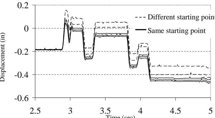
Figure 2.13 Displacement vs. Time, Different start points 59
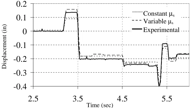
Figure 2.14 Displacement vs. Time, Specimen 1 61
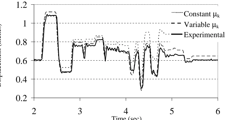
Figure 2.15 Displacement vs. Time, Specimen 2, Start from Center of Tile 63 Figure 2.16 Displacement vs. Time, Specimen 2, Start from Right Side of Tile 64
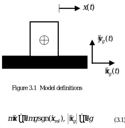
Figure 3.1 Model definitions 73
ix
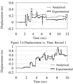
Figure 3.4 Displacement vs. Time, Record 1 82
Figure 3.5 Displacement vs. Time, Record 2 82
Figure 3.6 Displacement vs. Time, Record 3 82
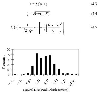
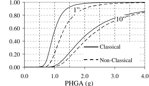
Figure 3.7 Peak Displacement vs. PHGA, Classical Friction, µ = 0.20 84 Figure 3.8 Histogram of the Natural Log of the Peak Displacement vs. PHGA,
classical Friction, µ = 0.20 86
Figure 3.9 Peak Displacement vs. PHGA, Classical Friction, µ = 0.20 89 Figure 3.10 Exceedance Probability vs. PHGA, Classical Friction, µ = 0.10 90
Figure 3.11 Acceleration vs. Time 91
Figure 4.1 Possible Variations in Static and Kinetic Friction 101
Figure 4.2 Model definitions 101
Figure 4.3, Peak Displacement vs. Source Distance, µ = 0.10 111 Figure 4.4, Peak Displacement vs. Shear Wave Velocity, µ = 0.10 112 Figure 4.5, Peak Displacement vs. Maximum Ground Velocity, µ = 0.10 113 Figure 4.6, Histogram of an Actual Data Set, PHGA=1g, µ = 0.10, n = 215 115 Figure 4.7, Actual CDF and Model CDF of a Data Set from Figure 4.6, PHGA = 1g,
Classical Friction µ = 0.10, n = 215 116
x
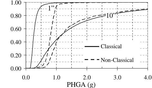
Figure 4.12, Fragility for Classical and NCS Friction of 0.10 123 Figure 4.13, Fragility for Classical and NCS Friction of 0.30 123 Figure 4.14, Fragility for Classical and NCS Friction of 0.50 124 Figure 4.15, Static Coefficient of Friction for NCS Friction of 0.1, 0.3 and 0.5 124 Figure 4.16, Hazard Curves, H(a), for the Four Locations 126 Figure 4.17, Hazard Curve with Two Best Fit Models, H(a), for San Francisco
CA 127
Figure 4.18, F’(a) for a slip of 2 inches, and NCK Friction of 0.10 127 Figure 4.19, Pf vs. Slip Displacement for Memphis TN, Classical and NCK
friction of 0.1, 0.3 and 0.5 129
Figure 4.20, Pf vs. Slip Displacement for Los Angeles CA, Classical and NCK
friction of 0.1, 0.3 and 0.5 129
Figure 4.21, Pf vs. Slip Displacement for San Francisco CA, Classical and NCK
frictions of 0.1, 0.3 and 0.5 130
Figure 4.22, Pf vs. Slip Displacement for Charleston SC, Classical and NCK
friction of 0.1, 0.3 and 0.5 130
Figure 4.23, Pf vs. Slip Displacement for Los Angeles CA, Classical and NCS
frictions of 0.1, 0.3 and 0.5 131
Figure 5.1: Plot of peak displacement vs. epicentral distance using a classical
friction of 0.10 138
Figure 5.2: Plot of peak displacement vs. epicentral distance using a classical
friction of 0.20 138
Figure 5.3: Plot of peak displacement vs. epicentral distance using a classical
xi
Figure 5.5: Plot of peak displacement vs. epicentral distance using a classical
friction of 0.50 140
Figure 6.1: Plot of peak displacement vs. shear velocity of local geology using
a classical friction of 0.10 143
Figure 6.2: Plot of peak displacement vs. shear velocity of local geology using
a classical friction of 0.20 144
Figure 6.3: Plot of peak displacement vs. shear velocity of local geology using
a classical friction of 0.30 144
Figure 6.4: Plot of peak displacement vs. shear velocity of local geology using
a classical friction of 0.40 145
Figure 6.5: Plot of peak displacement vs. shear velocity of local geology using
a classical friction of 0.50 145
Figure 7.1: Plot of peak displacement vs. peak ground velocity using a classical
friction of 0.10 147
Figure 7.2: Plot of peak displacement vs. peak ground velocity using a classical
friction of 0.20 148
Figure 7.3: Plot of peak displacement vs. peak ground velocity using a classical
friction of 0.30 148
Figure 7.4: Plot of peak displacement vs. peak ground velocity using a classical
friction of 0.40 149
Figure 7.5: Plot of peak displacement vs. peak ground velocity using a classical
friction of 0.50 149
Figure 8.1: Plot of peak displacements from dt = 0.005 seconds divided by the peak displacements from dt = 0.0001 seconds vs. PHGA using a classical friction of
xii
0.10 153
Figure 8.3: Plot of peak displacements from dt = 0.005 seconds and from dt = 0.0001
seconds vs. PHGA using a classical friction of 0.10 154
Figure 9.1: Plot of peak displacements without directionality and with directionality
of 80% vs. PHGA using a classical friction of 0.10 157
Figure 9.2: Plot of peak displacements without directionality and with directionality
of 80% vs. PHGA using a classical friction of 0.20 157
Figure 9.3: Plot of peak displacements without directionality and with directionality
of 80% vs. PHGA using a classical friction of 0.30 158
Figure 9.4: Plot of peak displacements without directionality and with directionality
of 80% vs. PHGA using a classical friction of 0.40 158
Figure 9.5: Plot of peak displacements without directionality and with directionality
of 80% vs. PHGA using a classical friction of 0.50 159
xiii
of 100000 seconds 173
Figure A.12: Fragility curves for a NCS friction of 0.30 and an initial time at rest
of 100000 seconds 174
Figure A.13: Fragility curves for a NCS friction of 0.50 and an initial time at rest
of 100000 seconds 174
Figure B.1: F’(a) for a classical friction of 0.10 175
Figure B.2: F’(a) for a NCK friction of 0.10 176
Figure B.3: F’(a) for a classical friction of 0.20 176
Figure B.4: F’(a) for a NCK friction of 0.20 177
Figure B.5: F’(a) for a classical friction of 0.30 177
Figure B.6: F’(a) for a NCK friction of .30 178
Figure B.7: F’(a) for a classical friction of 0.40 178
Figure B.8: F’(a) for a NCK friction of 0.40 179
Figure B.9: F’(a) for a classical friction of 0.50 179
Figure B.10: F’(a) for a NCK friction of 0.50 180
Figure B.11: F’(a) for a NCS friction of 0.10 180
Figure B.12: F’(a) for a NCS friction of 0.30 181
Figure B.13: F’(a) for a NCS friction of 0.50 181
Figure C.1: Log-log plot of USGS hazard data and model curve for Los Angeles
CA 182
Figure C.2: Log-log plot of USGS hazard data and model curve for San Francisco
xiv
Figure C.4: Log-log plot of USGS hazard data and model curve for Charleston
SC 184
Figure D.1: Log-log plot of USGS hazard data and model curve for San Francisco
CA 186
Figure D.2: F’(a) plot for a one inch displacement using a classical friction of
0.10 186
Figure E.1: Log-log plot of USGS hazard data and simplified curve for San Francisco
CA 191
Figure E.2: Log-log plot of hazard data with detailed curve for San Francisco
CA 191
Figure E.3: Plot of Pf per year vs. displacement using the standard and two-part
model for H(a) 192
Figure H.1: Example hazard curve, H(a) 211
Figure H.2: First example F’(a) distribution for a displacement of four inches with
a classical friction of 0.10 211
Figure H.3: Second example F’(a) distribution for a displacement of thirty inches
with a classical friction of 0.10 212
Figure H.4: Example realF’(a) distribution 212
Figure I.1: Fragility distributions for a one inch displacement with a NCS friction
of 0.10 and initial wait times of 10, 100, 1000, 10000, and 100000 seconds 215 Figure I.2: Fragility distributions for a five inch displacement with a NCS friction
of 0.10 and initial wait times of 10, 100, 1000, 10000, and 100000 seconds 215 Figure I.3: Fragility distributions for a ten inch displacement with a NCS friction
of 0.10 and initial wait times of 10, 100, 1000, 10000, and 100000 seconds 216
1
Chapter 1
Introduction
1.1 General Introduction
Unanchored bodies may respond in a variety of ways to seismic excitation. These response modes have been well defined by numerous studies. The two most common
2
minimized through the use of appropriate engineering analysis. The easiest way to minimize the likelihood of sliding damage is to design a safe zone around the object. A number of approaches have been developed over the years to assist in this process, but they each have issues which limit their applicability in a modern design environment. One of the principal limitations of these works is that they have utilized “classical” friction exclusively (µs,k are constant). While there are certainly a great many systems in existence which are well represented by this scenario, it is apparent from this research that it (classical friction) is not the only type of friction that engineers should be concerned with.
Another type of friction, referred to as non-classical (NC), has been identified in this research using experimental studies conducted with vinyl flooring tiles. Two distinct and independent types of NC friction have been identified. The first type of NC friction, referred to as NCK, affects the kinetic coefficient of friction, µk, only and is a function of the velocity of the sliding body relative to the floor. The second type of NC friction observed in this study, referred to as NCS, only affects the static coefficient of friction, and is a function of the time that the unanchored body has been at rest relative to the floor (or base). Bodies with either of these two types of friction will exhibit significantly different behaviors than bodies which behave in a classical fashion. Experimental studies have been conducted to
3
measurement devices. These are described in detail in subsequent chapters. The results of the seismic testing were generally very good meaning the analytical results matched experimental results quite closely.
4
1.2 Background
The sliding response of unanchored objects is traditionally considered in the context of “Classical” dry friction theory. This theory is summarized by the following three rules:
Rule #1: The limiting force of friction is directly proportional to the applied load (normal force), Ff = µFn (Ff= force of friction, Fn = normal force, µ = coefficient of friction)
Rule #2: The force of friction is independent of the apparent area of contact. Rule #3: Kinetic friction is independent of the sliding velocity.
5
the array of behaviors being observed and they discussed improved models, techniques and procedures for obtaining the parameters in these models.
In civil engineering, one important application of frictional behavior is associated with earthquake excitation since unanchored objects such as desks, scaffolding, or cabinets may slide during an earthquake and damage adjacent equipment. To model this sliding behavior, several questions about friction must be asked: Are the coefficients equal and constant with respect to, for example, velocity (figure 1.1a)? Are they constant yet not equal (figure 1.1b)? Or are they governed by some other relationship (figure 1.1c)?
Figure 1.1 Possible Variations in Static and Kinetic Friction Once these relations are established, the sliding response to any number of scenarios can be determined by numerically integrating the difference between the ground acceleration and the acceleration response of the unanchored object and applying the
?
?
Fs
Fk,
Fk
Fs
a) Friction b) Friction c) Friction
6
appropriate boundary conditions. The unanchored body’s acceleration response is determined by the frictional characteristics of the system in question.
The sliding motion for a rigid body on a horizontal surface which is undergoing horizontal acceleration is traditionally governed by the following differential equation, see figure 1.2,
g
x
x
mg
x
m
&
&
=
µ
sgn(
&
rel),
&
&
g>
µ
(1.1)where x(t) and x&rel(t)are the absolute displacement and relative velocity of the body, )
(t
x&g
& is the horizontal ground acceleration, x&& is the absolute acceleration of the body, y&&g(t)
is the vertical ground acceleration, µ is the coefficient of friction, m is the mass of the body and g is the acceleration due to gravity. Sgn is the signum function where sgn( ) is 1 if the argument is positive and -1 if negative. This formulation assumes no vertical component of acceleration, but it is simple to modify the relevant coefficient of friction if this component of acceleration does exist as shown in equation 1.2. Where needed, the friction coefficients are modified directly instead of the normal force.
+
=
g
y
gk s k s
&
&
1
, *
,
µ
7
)
(
t
x
&
y
&
g(
t
)
x
&
&
g(
t
)
Figure 1.2 Model definitionsA MATLAB program, SLIDE3, was written to numerically determine the sliding response an unanchored body in lieu of solving the differential equation in closed form. Typically a time step, ∆t, which ranged from 0.005 to 0.0004 seconds was used depending upon the application. The results from each successive step are used to calculate the position of the block relative to the base (using a rectangular rule).
1.3 Literature Review
8
and constant. Second, the seismic event consisted of a single, rectangular pulse. And third, there was no vertical component to the seismic event. By applying these constraints, a closed form solution was derived to predict the displacement for the given scenario. While this solution is certainly simple to use, it is probably not rigorous enough by modern standards to offer more than a rough estimate, and this is only when the three assumptions are not grossly violated. For instance, ignoring the vertical component alone can lead to very large errors. With vertical motion a body can potentially slide even though µs is greater than the peak horizontal ground acceleration (PHGA) if the pulse coincides with a strong downward motion. Many systems also demonstrate a µk which is less than µs. In this case,
overestimating µk will lead to an underestimate of the relative displacement. And lastly, a single rectangular pulse rarely represents a seismic event well. A modified version of this work was presented in 2000 by Choi which used a triangular pulse [6]. While this was an improvement, it was hindered by many of the same assumptions as the original.
In the years following Newmark’s work, civil engineers began to experimentally verify the sliding behavior of unanchored bodies. Experimental studies such as these are vital in order to verify the models and assumptions. The earliest of these studies is the work of Aslam et al. in 1975 [7]. Using the shake table at UC-Berkeley, they were able to
9
kinetic friction (equal and constant here) which are still used extensively today. The most useful of these is to apply a continuous, fixed sine wave input (acceleration) to the sled and examine the response of the object. The acceleration of the body (a direct indicator of µ) was observed and recorded. This work was also the first to utilize recorded earthquakes with both horizontal and vertical motions. Their frictional measurements were thoroughly tested and reconciled with seismic analyses. In general, the results were good, but there were some shortcomings. First, the use of a single parameter model (µs = µk), while simplifying the analysis, is not very realistic for many applications. Several systems have a µk which is 10-20% less than µs or behave in a different fashion altogether. Secondly, the data acquisition rate of 100 points per second is generally insufficient to represent accurately the acceleration behavior of the bodies during sliding. While they were limited by existing technology, a higher sampling rate is critically important in monitoring systems to demonstrate more complicated frictional behavior.
10
examination and the sliding results were quite varied. The percent differences in peak displacement ranged from 10% to over 100% and, in most cases, did not appear to be repeatable. It was assumed in that study that µs and µk were constant and equal and this assumption may have led to the difficulty in achieving reconciliation between measured and computed results.
The next approach, by Shao, used 75 real uniaxial seismic records to generate a set of conditional probability curves for a given classical friction model and PHGA [9]. These curves presented the 84th percentile probability displacement for a given PHGA. As a part of the study, Shao also investigated the impact of vertical motion and the use of artificial earthquakes. It was found that artificial earthquakes yielded very conservative results and, when using these artificial earthquakes, the effect of vertical motion was seen to increase displacements by less than 10%. While this study did not address slip in a PRA context, it is still useful because of its many sound observations.
11
friction. This was only slightly better. Their experimental data were compared to fragility curves for verification and the results were mixed. One interesting observation is that some of their fragility curves actually crossed. This seems highly unlikely as it implies that a lower PHGA will yield a higher displacement. While this is certainly possible for individual seismic time-histories, it seems unusual for a large set of earthquakes (90 in total) as was used in their study. Ultimately these problems lessen the usefulness of the study to the engineering community.
The work of Chong et al. was followed in 2003 by an analytical study which recycled much of Chong’s earlier work. That study, by Garcia et al., appears to have utilized Chong’s artificial earthquakes developed from the National Earthquake Hazard Reduction Program (NEHRP) guidelines for the seismic design of structural frames [10, 11]. Ninety artificial earthquakes (using SIMQUAKE), generated from a design response spectrum, were used as their population for analysis [12]. From this population, peak displacements were calculated and fragility curves developed for a range of classical coefficients (µs = µk) and limit states corresponding to specific displacements. The final product was essentially the same set of fragility curves relating displacement to PHGA as seen in Chong et al., although none of these published curves crossed.
12
6]). SLIDE2 is important in that it is apparently the first sliding program to incorporate independent µs and µk values. The frictional system used in his experiments was metal sliding on metal. The frictional parameters, µs and µk, were measured manually and
mechanically using static pull tests, incline tests, dynamic tests (with a sinusoidal input), and a pulley test. A series of seismic tests on a shake table were also conducted to check SLIDE2 and the system parameters. The results were mixed, though somewhat better than in
Nigbor’s study [8], which was expected since a more realistic model was used. Some of Warren’s tests worked out well, but several tests indicated a lack of repeatability. This was explained as a consequence of variations in friction and imperfections in the sliding surface. For example, µs and µk seemed to be dependent upon both direction and position. While that was not necessarily a novel observation, that relationship had not been seriously considered or examined previously in a civil engineering context. Another important result of his work dealt with the attempts to use best-fit solutions to generate values of µs and µk from seismic test data using a classical model. They found that it was difficult to generate consistently good results. Some results matched very well while others did not. These discrepancies were probably a consequence of using too simple a model for the system in question,
13
to demonstrate the variability of µ alone has proven to be very useful. A final suggestion by the author was to examine the relationship between the relative velocity and µk (for a total of five parameters!) for this system.
In 2005 a procedure for the design of sliding objects in nuclear facilities was proposed by the ASCE/SEI [14]. For sliding, take the friction at the 95% exceedance level and conduct time-history analyses using at least five earthquakes that satisfy the section 2.4 seismic requirements of the same ASCE guideline. Take the average of the peak slips that result and use this value as the “best-estimate.” Simpler alternative approaches are included as well and these are quite conservative. Unfortunately, this process is not risk consistent and few references were provided to support the appropriateness of their suggestions. It also does not distinguish between static and kinetic friction.
14
not very good. These values were based on best-fit regression analysis and were generally 20 to 30% lower than the measured values. Complicating their work were two obvious factors. First, the equipment being tested was tall and slender and began rocking in nearly every test. Second, since two of the units were mounted on flexible legs, the units “wobbled” without actually slipping. As Warren had done, they used best-fit µ values (which were significantly less than the directly measured values) to even get close to the experimental results.
Another work was published in 2005 by Chaudhuri and Hutchison [16]. This study focused on the sliding behavior of bench-top mounted equipment such as microscopes, monitors, and computers. Interestingly, their measurements of displacement were made using charged-couple device (CCD) imagery. While this is certainly an unobtrusive way to measure displacements and velocities, it is not clear that this approach is capable of
15
flat, the reverse is true. The results here were mixed. Some specimens demonstrated classical behavior during the low velocity inclined tests, but not during the high velocity tests. Another issue was the difference between results from the pull tests and the inclined tests. The values of µ from the inclined tests were generally less than the values measured during the pull tests. Which measured value should be used here? How can they all be correct in the classical sense? The authors attribute these variations into unnamed “state-dependencies” and used an average to generate the analytical results for the seismic validation phase. The percent error at the peak displacement between the analytical and experimental results varied from -40% to +40%. In their summary, it was concluded that µk was not entirely independent of the relative velocity but apparently no attempt was made to incorporate this observation into their model. This may be another example of where the strictures of the classical model limited the quality of the reconciliation results.
Ultimately, this work presented a series of fragility curves and suggestions for their application to structures different from their own. It is difficult to directly compare their results with the curves presented here because theirs were developed for a multi-story
structure and also accounted for the bench itself.
16
blocks (a total of six groups). The blocks were designed such that rocking responses would be excluded and three different frictional interfaces were used (carpet-steel, wood-steel, and PTFE (polytetrafluoroethylene)-steel. When measuring the frictional behavior, they used inclined tests and shake table based dynamic testing with sinusoidal input for measuring µk. Pull tests and inclined tests were used for determining µs. They assumed a two parameter model for this study. For µs, the results from the inclined tests were generally similar to those from the pull tests, the exception being the PTFE-steel interface blocks which were much less consistent overall than for the other systems. Three methods are described for the determination of µk. The first method utilized an inclined plane at a steep angle. From the acceleration data µk can be estimated and the results presented using this method were
consistently less than the results from the other methods. The second and third methods used a shake table to excite the specimens. Accelerometers were used in conjunction with a KRYPTON tracking system to monitor the specimens. Using up to nine sinusoidal inputs of varying frequency and amplitude per block, they determined µk using two distinct methods on the same cyclic test data. One method is based on the peak acceleration response of the block(s) and the second is based on the extrapolation of µk from the peak displacement of the block(s). Although why an indirect method based on displacements and a number of
17
from the body and a histogram is plotted of that data. In general, when there is a lot of sliding, the number of data points in this region will be significantly greater than the
ascending and descending portions. The concentration of data that will result represents the overall kinetic friction. This first method is satisfactory if µk behaves in a classical sense. The second method for extrapolating µk uses the peak relative displacements from the cyclic test data and seems cumbersome. Their measured and calculated values of µk are compiled by block size, and each pair is plotted using the values of µk as determined by both the displacement and acceleration methods. From these measurements, many of the blocks apparently have values of µk which are markedly different depending upon the calculation method. For instance, some blocks have a µk of 0.35 from the acceleration method, and 0.45 from the displacement method. If the model, methodologies and assumptions are correct, one would expect to get closer results from the two sets of data. The authors do not provide an opinion on which result might be preferred or what the cause of the difference might be. There was some minor rotation of the specimens, but data from the excessively rotated specimens was excluded. Also, these frictional results were consistently higher than the data from the inclined test data. This variation was not explained either.
18
unreasonable when dealing with a purely classical system. However, if there are significant dependencies between µk and other phenomena, such as relative velocity, the “averaging” approach on their data might not do a good job of representing the slippage that occurs during seismic conditions outside of the range of their excitations. We don’t know what range of relative velocities was observed during the testing and no seismic tests were conducted to validate the measurements. Also, none of the methods used here (or in any of the other studies for that matter) can identify and measure complexities in µs. The only evidence that complexities might exist is that the results were very inconsistent. Without the use of appropriate tests, however, such inconsistencies would likely be construed as
19
In summary, the availability of good experimental data on sliding behavior for realistic systems is lacking. Also, the published analytical studies to date have been largely inconclusive, inconsistent or only relevant to a limited set of circumstances. These issues should be addressed so that the engineering community can continue to safely design our structures.
1.4 Research Objectives and Organization of this Study
There were several objective to this project. The first was to successfully model the non-classical sliding behavior of an unanchored body under uniaxial and biaxial seismic conditions. This required preliminary testing to measure and quantify the friction. Upon completion, this phase was followed by seismic testing in which the measured frictional properties can be applied to the experimental behavior and the results compared. Ultimately, this was the most important aspect of this study because, regardless of how design
20
the number of variables present to only those necessary for the assessment. These
simplifications are discussed in chapters 3-6. Other topics are also included which may not be immediately relevant, but may be of interest to future studies. These are discussed in chapters 7, 8 and 9. The majority of the data used in the probabilistic analyses is included in the appendices. An example Pf calculation is also included in the appendices as is a
comparison of the various techniques used to calculate Pf.
There are a total of nine appendices, A through I. These appendices contain raw data, various analyses and some comparisons which will be of use in future studies.
Chapters 2, 3, and 4 have each been submitted, individually, to Earthquake Engineering and Structural Design for publication. The format used in this dissertation is largely consistent with their requirements. The exceptions being the numbering scheme for the subsections, tables and figures. These have been labeled to allow for easier locating by the reader of the dissertation.
The journal article contained in chapter 2 is a detailed description of the
21
The article which comprises chapter 3 attempts to settle an issue which has been discussed for many years in this field. The issue is the following: What is the impact of vertical motion on slip? Analyses are included which demonstrate that the effect of vertical motion is usually significant for a single seismic event. Analyses are also included which demonstrate that when working with large populations of earthquake records the effect of vertical motion is, surprisingly, quite small.
22
Chapter 2
This paper titled “Non-Classical Sliding Behavior of Unanchored Rigid Bodies “ by James Kevin Wilkin and Vernon C. Matzen
has been submitted to Earthquake Engineering and Structural Dynamics and is in review
23
Non-Classical Sliding Behavior of Unanchored Rigid Bodies
Abstract
A study of the uniaxial sliding response of unanchored rigid bodies on vinyl tile flooring to seismic loading was undertaken to determine if accurate predictions of this behavior could consistently be made if the tests were conducted in laboratory conditions. Currently the norm for reconciling such experimental work is to use a “classical” two
parameter mathematical model utilizing constant coefficients of static and kinetic friction, µs
and µk respectively. Results using this simple model have varied considerably. Before the
24
experimental work. Using constant values of µs and µk led to discrepancies of 15-20% or more between the experimental peak measurements and the predicted counterparts. Recognizing the above mentioned functional relationships allowed for the development of testing schemes which enhanced repeatability considerably. Incorporating the more detailed frictional model yielded results which were typically in error by less than 10% at the
maximum displacement. For these cases, the more detailed models provide much improved predictive capabilities.
2.1 Introduction
25
assumption is made that the body is configured so that rocking or a combined slide-rock behavior does not occur and thus the second question becomes irrelevant. If an object does slide, but has sufficient room between itself and adjacent objects, then sliding may not necessarily be of concern. But for objects with little room to slide it may be necessary to obtain an accurate estimate of the sliding distance and the first question becomes primary and the remainder of this paper is devoted to answering this question. For objects where slippage is to be minimized or prevented altogether, the bodies may need to be physically restrained, but this topic is beyond the scope of this paper.
If it is necessary to obtain an accurate prediction of sliding (usually meaning the maximum distance traveled), then it becomes necessary to have a mathematical model that adequately captures this behavior. A traditional model contains just two parameters, µs and
µk (or perhaps only one, µs) and considers only one dimensional motion. Whether or not this
26
simple two parameter approach is used most often, but with results that are sometimes questionable.
In some other fields, more complicated models are the norm. For several decades the tribological community have been using a more sophisticated (i.e. more than two parameters) approach to friction. There are a wide number of references dealing with the various
complexities [3, 4, 5, 6]. Examples include load dependent µs and µk, rest time dependent µs, velocity dependent µk of a linear or nonlinear nature, temperature dependencies and location or directional dependence to name a few. These models are used wherever friction is a primary design concern. This specifically applies to automotive and aerospace machinery such as turbines, combustion engines, and tires. These concepts are also applied to
components where friction induced vibrations are of concern such as brake pads and machine tools. In fact, judging by the tribology literature, the two parameter model commonly used in civil engineering may be the exception rather than the rule.
27
In this experimental seismic study, we have investigated the sliding behavior of two unanchored rigid bodies on vinyl flooring tiles. Vinyl tiles were selected because of their uniform properties and because they are widely used in commercial and emergency
buildings. Two sets of experiments were conducted, with different interface characteristics, and neither set of results was consistent with the “classical” two parameter model. The initial tests used techniques built around the two parameter model. The reconciliation results and repeatability using these techniques were not good. Upon closer examination of the actual behavior of the specimens, it was observed that many of their properties were not consistent with the classical scenario. Because of this observation, a set of tests was devised to
characterize this non-classical behavior in a consistent fashion. These characterizations were then incorporated into a MATLAB program designated SLIDE3, developed by our group for analysis and reconciliation. When using the techniques developed here, the experimental reconciliation results for the two test specimens improved significantly and were very repeatable.
2.2 Background and Literature Review
28
Rule #1: The limiting force of friction is directly proportional to the applied load, Ff = µFn (Ff = force of friction, Fn = normal force, µ = coefficient of friction)
Rule #2: The force of friction is independent of the apparent area of contact. Rule #3: Kinetic friction is independent of the sliding velocity.
Credit for these rules is generally attributed to Charles Coulomb, but other well known scientists such as Leonardo da Vinci, Guillaume Amontons, and Leonard Euler also contributed [5, 7]. Inherent in these rules is the existence of a separate coefficient of friction for both static and kinetic friction. The static coefficient, µs, is indicative of the amount of force required to initiate motion and the kinetic coefficient, µk, is indicative of the amount of force required to maintain slippage. Because the underlying mechanisms of friction are not completely understood, their characterization requires empirical analysis. A great deal of experimental work was carried out by tribologists and mechanical engineers studying the frictional properties of mechanical components in the early 20th century. Interestingly, they recognized that the classical model was not always sufficient to represent the array of behaviors being observed and they discussed techniques and procedures for obtaining the parameters in these models.
29
friction must be asked: Are the coefficients equal and constant (figure 2.1a)? Are they constant yet not equal (figure 2.1b)? Or are they governed by some other relationship (figure 2.1c)?
Figure 2.1 Possible Variations in Static and Kinetic Friction
Once these relations are established, the sliding response to any number of scenarios can be determined by numerically integrating the difference between the ground acceleration and the acceleration response of the unanchored object and applying the appropriate
boundary conditions. The specimen’s acceleration response is determined by the frictional characteristics of the system in question.
The sliding motion for a rigid body is traditionally governed by the following differential equation, see figure 2.2,
?
? Fs
Fk,
Fk Fs
a) Friction b) Friction c) Friction
30
g
x
x
w
x
m
&
&
=
µ
sgn(
&
rel),
&
&
g>
µ
where x(t) and x&rel(t)are the absolute displacement and relative velocity, x&&g(t)is the ground acceleration, w is the weight of the body and g is the acceleration due to gravity. Sgn is the signum function where sgn( ) is 1 if the argument is positive and -1 if negative. This formulation assumes no vertical component of acceleration.
x
(
t
)
)
(
t
x
&
g&
Figure 2.2 Model definitions
31
For some regular or steady state signals the displacements can be expressed in a closed form [8, 9]. For transient signals, such as an earthquake, however, the response must be discretized and analyzed over a series of very small time steps for the duration of the excitation event. If the event includes a vertical component of acceleration, then this too must be accounted for in the analysis. When sliding behavior is part of the design
considerations, accurate analytical models are clearly important; if the sliding behavior of an unanchored body cannot be predicted accurately, then excessively conservative design rules to account for our uncertainty must be used.
A variety of test methods have been developed to measure the frictional properties of classical (two parameter) systems. These methods, using devices known generically as tribometers, can be simple in the case of classical models (used extensively in the civil engineering literature) or more elaborate for the more complex models. The most common of the simple methods is the horizontal pull test. In this method an unanchored body is pulled along the surface using a cable. The cable will have either a spring scale or a load cell placed along its length to monitor the load at any instant. This method can be used to
32
the relationship between this angle, θs, and the static friction is given by µs = tanθs. Two modified versions of this test have been used recently in other studies. One version begins with the platform at a steep angle, i.e. greater than θs. Accelerometers are used to measure the acceleration of the body as it slides down the tilted platform. Theoretically, this data can be used to find µk, but, at least in one instance, the trial results were not satisfactory [10]. A second modification also begins with the platform already at a steep angle, greater than θs. The specimen is released and its displacement is measured, rather than acceleration, as its slides down the platform [11]. From the displacement data, the velocity, acceleration and µk are determined by numerical differentiation. The angle of tilt can be adjusted to achieve higher or lower velocities as needed. While these procedures have the capability to
recognize variations in µk, they are not sufficient to rigorously identify any complexities that may exist.
One of the first civil engineering studies to deal with the displacement of unanchored objects was published in 1965 by Newmark [8]. This work dealt with earthen dams, but the principles are applicable to sliding in general. In his study three major assumptions were made with respect to the system parameters. First, µs and µk were equal and constant (a one parameter model). Second, the seismic event was comprised of a single, rectangular pulse. And third, there was no vertical component to the seismic event. By applying these
33
scenario. While this solution is certainly simple to use, it is probably not rigorous enough by modern standards to offer more than a rough estimate and this is only when the three
assumptions are not grossly violated. For instance, ignoring the vertical component alone can lead to very large errors. With vertical motion a body can potentially slide even though
µs is greater than the peak horizontal ground acceleration if the pulse coincides with a strong
downward motion. Many systems also demonstrate a µk which is less than µs. In this case, overestimating µk will lead to an underestimate of the relative displacement. And lastly, a single rectangular pulse rarely represents a seismic event well. A modified version of this work was presented in 2000 by Choi which used a triangular pulse [9]. While this is an improvement, it is hindered by many of the same assumptions as the original.
34
of µ) was directly observed and recorded. This work was also the first to use recorded earthquakes with both horizontal and vertical motions with respect to sliding behavior. Their frictional measurements were thoroughly tested and reconciled with seismic analyses. In general, the results were good, but there were some shortcomings. First, the use of a single parameter model (µs = µk), while simplifying the analysis, is not very realistic for most applications. Many systems, at a minimum, have a µk which is 10-20% less than µs. Secondly, the data acquisition rate of 100 points per second is generally insufficient to represent accurately the acceleration behavior of the bodies during sliding. While they were limited by existing technology, a higher sampling rate is critically important in monitoring systems to demonstrate more complicated frictional behavior.
35
assumption may have led to difficulty in achieving reconciliation between measured and computed results.
The next experimental sliding study was published by Warren in 2000 [14]. This work was conducted to validate two computer programs (called SLIDE, and later SLIDE2 [15, 9]). SLIDE2 is important in that it is apparently the first sliding program to incorporate independent µs and µk values. The frictional system used in his experiments was metal sliding on metal. The frictional parameters, µs and µk, were measured manually and
mechanically using static pull tests, incline tests, dynamic tests (with a sinusoidal input), and a pulley test. A series of seismic tests on a shake table were also conducted to check SLIDE2 and the system parameters. The results were mixed, though somewhat better than in
36
probably a consequence of using too simple a model for the system in question, especially when considering the repeatability issues. No further attempts were made to fully reconcile the results. It certainly would have required the use of at least two more parameters in the model (location and direction) to obtain consistent repeatability. That they were able to demonstrate the variability of µ alone has proven to be very useful. A final suggestion by the author was to examine the relationship between the relative velocity and µk (for a total of five parameters!) for this system.
37
actually slipping. As Warren had done, they used best-fit µ values (which were significantly less than the directly measured values) to even get close to the experimental results.
Another work published in 2005 by Chaudhuri and Hutchison [11]. This one focused on the sliding behavior of bench-top mounted equipment such as microscopes, monitors, and computers. Interestingly, their measurements of displacement were made using charged-couple device (CCD) imagery. While this is certainly an unobtrusive way to measure
displacements and velocities, it is not clear that this approach is capable of extracting reliable acceleration data from the sliding object, and as mentioned before, acceleration data is extremely useful for characterizing friction. Their test procedures included both slow pull tests and inclined plane tests. The incline tests were conducted at both high and low velocities (depending upon the angle of inclination). The CCD cameras were used in both cases to monitor displacement and velocity to assist in extracting the relevant frictional behavior. From the shape of the relative velocity curve (plotted against time) it is possible to determine if the system behaves in a classical fashion. If the slope of this curve is constant,
µk is constant and the two parameter model is satisfied. If the slope is not constant, the
38
the pull tests. Which measured value should be used here? How can they all be correct in the classical sense? The authors attribute these variations into unnamed “state-dependencies” and used an average to generate the analytical results for the seismic validation phase. The percent error at the peak displacement between the analytical and experimental results varied from -40% to +40%. In their summary, it was concluded that µk was not independent of the relative velocity but apparently no attempt was made to incorporate this observation into their model. This may be an example of where the strictures of the classical model limited the quality of the reconciliation results.
In 2007 a report was published by Kafali et al. which described experiments with the sliding behavior of rigid wooden blocks [10]. This study describes their methods for
39
determination of µk. The first method utilized an inclined plane at a steep angle. From the acceleration data µk can be determined and the results presented using this method were consistently less than the results from the other methods. The second and third methods used a shake table to excite the specimens. Accelerometers were used in conjunction with a KRYPTON tracking system to monitor the specimens. Using up to nine sinusoidal inputs of varying frequency and amplitude per block, they determined µk using two distinct methods on the same cyclic test data. One method is based on the peak acceleration response of the block(s) and the second is based on the extrapolation of µk from the peak displacement of the block(s). Although, why an indirect method based on displacements and a number of
assumptions is required when we can directly use the acceleration data was not explained. The acceleration based method essentially combines all of the recorded acceleration data from the body and a histogram is plotted of that data. In general, when there is a lot of sliding, the number of data points in this region will be significantly greater than the
40
apparently have values of µk which are markedly different depending upon the calculation method. For instance, some blocks have a µk of 0.35 from the acceleration method, and 0.45 from the displacement method. If the model, methodologies and assumptions are correct, one would expect to get closer results from the two sets of data. The authors do not provide an opinion on which result might be preferred or what the cause of the difference might be. There was some minor rotation of the specimens, but data from the excessively rotated specimens was supposedly excluded. Also, these results were consistently higher than the data from the inclined test data. This variation was not explained.
41
tests, however, such inconsistencies would likely be construed as “randomness” and “state-dependence”. In addition, the validity of their µk analysis depends on having a relatively large amount of data from the actual sliding phase. Otherwise the sliding data may
inadvertently be lumped in with static data (where the relative velocity is zero) which would skew the analysis. Another more technical issue is in the construction of the block’s friction system. Why was the carpet mounted to the bottom of the blocks? This being the case, the load is distributed over the entire block/carpet bottom and there are no edge effects from sharp corners pressing into the carpet. Surely this will affect the coefficient of friction. This type of study is interesting in a statistical sense, but it would have been much more useful if there had been an analytical component with some attempt at reconciliation.
42
several of the systems tested, it has been demonstrated conclusively in other fields that this is simply not the case for many frictional systems.
2.3 Experimental Work
An experimental study at North Carolina State University by Wilkins and Matzen in 2007 [17] attempted to resolve some of these issues by examining, in detail, the frictional characteristics of two different unanchored rigid bodies, with two different base
configurations, on vinyl tiles. There were two goals for this work; one was to develop a consistent and reliable set of data for the one-dimensional sliding behavior of a rigid body subjected to various types of excitation, and the other was to create a robust mathematical model that would be capable of accurately simulating the experimental behavior. As described earlier, it is not possible to design the experiments without knowing the specific aspect of sliding that was to be measured. Thus, in this project the testing and modeling work proceeded concurrently, with each part influencing the direction the other would take. The details of this work are discussed below.
43
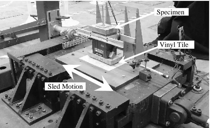
was wooden and four metal slides were mounted to it, see figure 2.4. The slides are similar to those found in commercial applications such as tables and desks, and these slid directly on the vinyl tile during testing. The total weight of each assembly was approximately 35 lbs and both were approximately 10 inches tall. The specimens were designed with a wide base and a low center of gravity to limit the possibility of rocking or slide-rocking. A pair of thin aluminum guide rails was mounted to the sides of the specimen. These rails, guiding the specimen between rows of roller bearings, constrained the specimens to uniaxial motion. The clearance between the rails and bearings was adjusted to ensure that the bearing had a negligible impact on the sliding.
The specimen and tile were placed on the sled of an ANCO shake table which was driven by a 20 kip hydraulic actuator, see figure 2.5. The actuator, which is managed by a Gardner Systems controller, receives an analog signal from a desktop computer using LABVIEW software. This system allows any displacement within +/- 3 inches and a velocity of up to 40 inches/sec. The tile(s) were glued to the top of the sled.
44
specimen behaved so differently, they will be treated separately in what follows. Following the sections on tests to obtain the frictional characteristics, a series of seismic tests will be described.
Figure 2.3 Test Specimen One, Metal base
Figure 2.4 Test Specimen Two, Metal slides
Wood Base Slides Guide Rails
Guide Rails
45
Figure 2.5 Specimen Two on the Shake Table
2.4 Specimen One Frictional Measurements
The first specimen slid atop the vinyl tile directly on its steel base, see figure 2.3. The base was machined flat and the bottom edges were chamfered to prevent them from cutting into the tile. The first step was to measure the static coefficient of friction. This task can be done in a number of ways. One is to use a set of weights hanging on a cord which goes over a pulley and is attached to the specimen. When the force from the weights exceeds the critical value, µsFn, (where Fn is the normal forces) the specimen will begin to move. One may also tilt the base of the body until sliding begins. The angle at which sliding occurs can
Specimen
Vinyl Tile
46
be used to determine µs, i.e. µs = tanΘ. Another technique used a hand cranked screw actuator to move the body across the tile. A load cell mounted between the actuator and the body measures the force continuously as the hand crank is turned. A fourth technique which we have used is an adaptation of the previous method. The entire frictional system, specimen and tile, is placed on the shake table sled as in a seismic test. The screw actuator is mounted to an external fixed frame which is independent of the sled movements. A series of very small displacements (around 0.1”) are sent to the sled in regular intervals (approximately 1 sec.). The body, which is fixed to the screw actuator and load cell, is restrained from moving relative to the fixed external reference frame as the sled displaces underneath it. As the sled moves, the frictional force between the body and the tile is recorded continuously. The static coefficient of friction is determined by dividing the force measured at the initiation of sliding by the weight of the body. A fifth technique uses a sinusoidal displacement of the sled to shake the unrestrained specimen until it slips. The acceleration of the body is measured continuously and µs and µk can be determined from this response. These techniques all work well at representing µs as long as it is constant (or nearly so). The fourth method is
47
Based on the above testing regime, µs appeared, in fact, to vary significantly. The observed variation was sometimes extreme and the test methods described above were not useful in deciphering any patterns. Only after examining the behavior of the rigid body under seismic excitation did a pattern emerge.
This variation is clearly evident in the acceleration record from the seismic test in figure 2.6. When the body is not moving relative to its base, the acceleration of the body and sled should be identical. As soon as the base acceleration exceeds a critical value, µsg, the curves diverge (located by the black circles on figure 2.6). The value of acceleration at which this divergence begins is a measure of µs. In this test, the first slippage occurs at approximately 1.40g’s, which corresponds to a µs of 1.40 (yes, greater than 1.0). The second slip occurs at an acceleration of 0.50g’s (µs = 0.50). Clearly, the value of µs is not constant. Recognizing this, it is necessary to first determine what the characteristics of the motion µs depends upon, and then determine the relationship between the coefficient and these
48
To determine the relationship between µs and rest time, a new test was devised. The specimen was placed on the sled and subjected to series of short, strong “steps”. The actual signal is a series of very short duration (approximately 0.01 seconds) stepped displacements. The individual steps are less than a tenth of an inch and the total displacement of the entire signal is nearly an inch. These individual steps were strong enough to ensure slippage, but short enough to limit the total displacement. The steps were temporally spaced from 10 to 0.1 seconds apart and were repeated in the opposite direction. The results from one such test are shown in figure 2.7. There is a clear relationship between µs and the time at rest. This can be reasonably approximated by a log curve using EXCEL solver, see figure 2.7. There was occasionally some dependency of the data on the direction of slip based on our tests. This directional dependency varied daily between tiles and sometimes between tests. Another outcome from this test was that this particular phenomenon is generally repeatable and insensitive to load rate.
49
was treated as such during our analyses. The final results of the seismic tests using Specimen One are discussed in the analysis section.
-1.5
-1
-0.5
0
0.5
1
1.5
33
33.1
33.2
33.3
33.4
Figure 2.6 Acceleration vs. Time
y = 0.058Ln(
∆
t) + 0.6727
0.4
0.5
0.6
0.7
0.8
0.9
0.01
0.10
1.00
10.00
100.00
Figure 2.7 Coefficient of Static Friction vs. Time at Rest
A cc el er at io n ( g ) Time (sec) g
x
&
&
bodyx
&
&
gx
&
&
bodyx
&
&
Time at Rest, ∆t (sec), log scale
µ
s50
2.5 Specimen Two Frictional Measurements
Specimen Two used four chrome plated slides attached to the bottom of the wooden plate (see figure 2.4). They are very similar to those seen on workbenches, office chairs, tables and desks. These slides rested directly on the vinyl tiles. After concluding the study of Specimen One, we sought to determine if µs was variable for this base configuration. Using techniques discussed with respect to Specimen One, it was determined that µs was, in this case, nearly constant. The primary source of variation in µs was usually related to slip direction, although different tiles could also vary slightly as with Specimen one. The principal difference between Specimens one and two is related to the kinetic coefficient of friction, µk. While µk for Specimen One was constant, µk for Specimen Two was not. As seen in figure 2.8, the specimen slips three times in this 0.3 second interval (indicated by the white circles) as indicated by the diverging acceleration curves of the body and the table. The ground acceleration, x&&g, at each divergence is very nearly 0.25g, or µs = 0.25. Note also that the time of rest between slippage varies even as µs remains constant. Another observation: if
µk were constant, the acceleration record of the specimen would remain constant immediately
after initiation of slip, but the specimen acceleration, x&&body, continues to rise as the relative
51
velocity is decreasing and the acceleration of the body is decreasing as well. When the relative velocity is zero, the curves merge until the next slip. From the third divergence, µk appears to vary from 0.25 to 0.35 and it appears to be directly related to the relative velocity between the sled and the specimen.
Figure 2.9 represents a view of the final peak from figure 2.8. The sled and specimen accelerations have been plotted and a curve based on the classical model, x&&body−classical, of the specimen has been plotted. The classical curve remains at -.25g until the relative velocity of the sled and specimen reaches zero. Because this moment in time is later for the classical curve than in reality, the classical model would predict a larger displacement and velocity error. The actual error will vary depending on the magnitude of the ground acceleration, x&&g. For strong earthquakes, using the classical model will probably result in significant
conservatism.