Power Amplifier Linearization Using Multi-Stage Digital Predistortion Based On Indirect Learning Architecture

(1)

Copyright to IJIRSET www.ijirset.com 216

Power Amplifier Linearization Using

Multi-Stage Digital Predistortion Based On Indirect

Learning Architecture

Sreenath S 1, Bibin Jose2, Dr. G Ramachandra Reddy3

Student, SENSE, VIT University, Vellore, Tamil Nadu, India1,

Student, SENSE, VIT University, Vellore, Tamil Nadu, India2, Senior Professor & Dean, SENSE, VIT University, Vellore, Tamil Nadu, India3

ABSTRACT: Power amplifiers (PA) are one of the essential components of communication systems and are nonlinear in nature. The nonlinearity creates in band and out of band distortions. To linearize a PA the cost effective method is use of digital predistortion. In this paper we propose a multi stage algorithm for digital predistortion using QR Decomposition. The coefficients are estimated using Indirect Learning Approach (ILA). In multi stage ILA the predistortion is implemented in two or more stages as compared to the single stage implementation of the conventional ILA approach. The multistage predistorters can achieve the same performance or even better performance than single stage predistorter depending on the power amplifier with lower complexity. The complexity is measured by the number of coefficients required for the identification of the predistorter. The performance of the multistage ILA is evaluated in terms of improvement in spectral regrowth suppression when an OFDM signal is given as input signal. Wiener-Hammerstein model is used for PA modelling.

KEYWORDS: Power amplifiers; Digital predistortion; Wiener-Hammerstein model; Indirect Learning Approach (ILA); Least Squares method; QR Decomposition.

I. INTRODUCTION

Power amplifiers are one of the essential components of a communication system and are inherently nonlinear in nature. This nonlinear nature produces in-band distortion (BER performance deterioration) and out-of-band distortion (Spectral regrowth beyond signal bandwidth) [1, 2]. For low power amplifiers and narrow band input signals, the power amplifiers can be modelled as memoryless nonlinearity [3]. In memoryless PA the current output of PA depends only on current input to PA. With the use of wideband signals such as OFDM or WCDMA in communications the power amplifier tend to exhibit memory effects. The memory effects arise due to the presence of thermal constants of active devices which are having frequency dependent behaviours. Now the current output of PA not only depends on current input to PA but also the past input values to PA. The memory effects further deteriorate the transmitted signals resulting in more out-of-band and in-band distortions.

(2)

of that of PA (see Fig.1.1). Thus the cascaded predistorter-PA system can work as a linear system and PA can be driven more to the high efficiency saturation region without compromising much on linearity.

Fig.1.1 Digital Predistortion

For the realization of DPD we use the indirect learning approach (ILA) which requires only the input and output of PA for estimating the coefficients [7]. In ILA first we estimate a post-distorter and this post-distorter is then used as a predistorter. The memory polynomial model is usually used for the modelling of DPD. The nonlinearity order and memory depth of the memory polynomial PD depends upon the PA nonlinearity to be compensated and varies with the PA. There is always a limitation on the maximum performance that can be achieved by this conventional ILA-DPD approach. Once the ILA-DPD system converges to the best possible solution, there is no substantial improvement in the performance with any subsequent increase in nonlinearity order or memory depth.

In this paper we propose a multi stage ILA for digital predistortion which is having less computational complexity for the parameter estimation, as compared with the conventional ILA approach. The nonlinearity of PA is compensated using two or more than two stages in multistage ILA. Each stage can be modelled using a lower order memory polynomial and thus having low computational complexity. The identification complexity for conventional as well as multi-stage ILA is measured by computing the number of multipliers needed.

The remainder of this paper is organized as follows. Section II gives an overview of Wiener-Hammerstein model and section III gives the brief description related to conventional indirect learning architecture (ILA). Section IV presents the proposed identification algorithm for multi-stage PD. In Section V simulation results for proposed algorithm is presented and discussed. Finally Section VI concludes the paper.

II. WIENER-HAMMERSTEINMODEL

The Wiener-Hammerstein model [8] is a three-box behavioural model. The Wiener-Hammerstein Model is modelled as a LTI system followed by a memoryless nonlinearity, which in turn is followed by another LTI system (see Fig.1.2). This type of configuration is generally used in satellite communication channels, where the power amplifier at the satellite transponder is driven near saturation to exploit the maximum power efficiency for the downlink [9].

Fig.1.2 Wiener-Hammerstein Model

The subsystem model can be described as

(3)

Copyright to IJIRSET www.ijirset.com 218 ( ) = ( )

,

| ( )|

( ) = ( − ) (1)

where, = [ , . . , ]and = [ , . . , ] are the impulse response values of LTI systems before and after memoryless nonlinearity respectively and = [ , , . . , ] are the coefficients of the memoryless nonlinear block.

III. CONVENTIONALINDIRECTLEARNINGARCHITECTURE(ILA)

The single stage PD identification using ILA is given in Fig.2.1. A post inverse of the PA is estimated and used as PD. The feedback path labelled “Predistorter Training” (block A) has ( ) is its input in case of memoryless PA and ( ) in PA with memory, where is the intended power amplifier gain, and ̂( ) as its output. The actual predistorter is an exact copy of the feedback path (copy of A); it has ( ) as its input and ( ) as its output. Ideally, we would like ( ) = ( ),

which renders ( ) = ̂( ) and the error term ( ) = ( )− ̂( ) = 0. Given ( ) and ( ), this structure enables us to find the parameters of block A directly, which yields the predistorter. The algorithm converges when the error energy

|| ( )|| is minimized [6].

Fig.2.1 Conventional Indirect Learning Approach

A. Memory polynomial Predistorter Design

The memory polynomial predistorter [10] in the training branch can be described by

̂( ) = ( − )| ( − )| (2)

(4)

terms gives a rich basis set and can provide good predistortion results without using higher order polynomials [11]. Based on a set of PA input { ( )} and output { ( )} measurements, the solution can be obtained for the predistorter coefficients, = , , … . . Once the coefficients are found then they are plugged into the predistorter:

( ) = ( − )| ( − )| (3)

The memory polynomial predistortion requires generation of a new sequence from power amplifier output which is given as,

( ) = ( − ) ( − ) (4)

at convergence, we should have

= (5)

where

= [ (0), (1), … . , ( −1)] = , , . . . , , … , …

= (0), … … , ( −1)

= , … . . , … , , . . ,

The least squares solution for (5) is given by

= ( ) (6)

where (. ) denotes complex conjugate transpose. But implementing matrix inverse in real time applications is not feasible and the digital signal processor precision may impact the accuracy of the resulting matrix inverse which may reduce the performance of predistorter. For estimating the inverse we go for pseudo inverse methods like Singular Value Decomposition (SVD), QR Decomposition etc. SVD and QR give same results but the computations required to find the predistortion coefficients in SVD is high compared to QR Decomposition since SVD requires the computation of Eigen Values and Eigen vectors.

B. QR Decomposition

Mathematically any matrix A can be written as

= (7) where R is an upper triangular matrix with > 0 and Q is an orthogonal matrix. An orthogonal tensor Q satisfies the necessary and sufficient conditions of = . For a square matrix A, the simultaneous equations = can be solved by the QR decomposition, = as [12].

=

= ( = )

= (8)

Solving the equation 8 using back substitution gives the estimates for .

IV.MULTI-STAGEINDIRECTLEARNINGARCHITECTURE

(5)

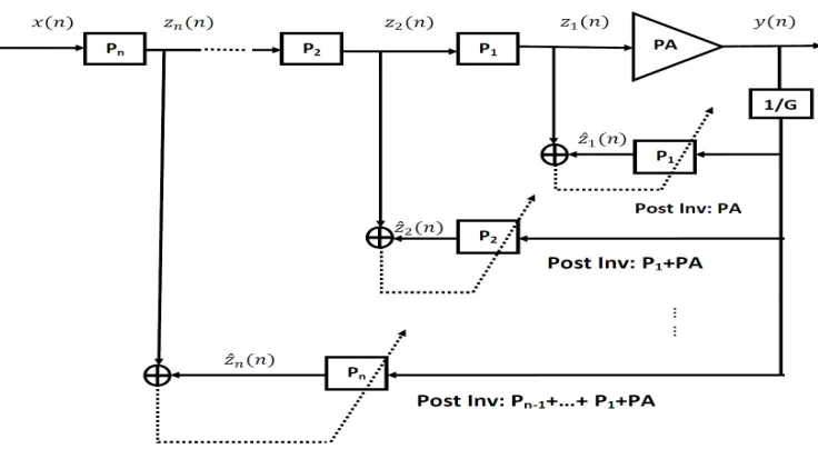
get convergence. The block diagram of the multistage ILA is shown in Fig 4.1. For identification of each stage more than more than one system level iteration is needed. After the convergence of a stage we can proceed with the identification of next stage.

Fig 4.1. Indirect learning architecture of a multi-stage DPD

Fig. 4.2 describes this algorithm for a 3 stage DPD, where the dark boxes represent the stages that are currently being identified. For the first iteration stage 1 is identified. In second iteration, the stage 1 cascade with PA is considered for linearization and estimates the second stage. This process continues and in third iteration stage 3 of DPD is identified.

Fig 4.2. Graphical illustration of Multi-stage ILA algorithm with 3 stage PD.

V. SIMULATIONRESULTS

In this section we present and analyse the simulation results for multi-stage ILA. The two LTI systems in W-H model are given as ( ) = 0.8 + 0.1 and ( ) = .

. where ( ) denotes the LTI block before memoryless nonlinearity and

( ) is the LTI block coming after memoryless nonlinearity. The memoryless nonlinearity is taken as Rapp Model. The Rapp Model is a memoryless power amplifier model developed for solid-state power amplifiers (SSPA). The input output relation of Rapp model is given as

=

1 + | |

/( ) (9)

(6)

64 with 56 subcarriers used for transmitting data. The OFDM is oversampled by a factor 4 and is then passed through a raised cosine filter having a roll off factor = 0.5. For simulations the smoothness factor P of Rapp model is taken as 2 and is taken to be 1V. Table 5.1 shows the results for a PA modelled as Wiener-Hammerstein model. and are highest order of memory polynomial and maximum memory depth respectively. The CC of two-stage ILA has been normalized with respect to conventional ILA.

Table 5.1:Identification of Memory Polynomial Predistorter using different approaches

Parameters Without DPD Conventional ILA Multi-stage ILA

Index array for

Nonlinearity and Memory

NA K=[1,2,3,4,5]

Q=[0 ,1,2,3,4,5,6,7,8,9,10]

Stage 1:

K=[1,2,3,4,5], Q=[0,1,2,3,4] Stage 2:

K=[1,2,3,4,5], Q=[0,1,2] Number of Coefficients NA 55 Stage 1: 20

Stage 2: 15 Normalized Complexity NA 1 Stage 1: 0.3636

Stage 2: 0.2727

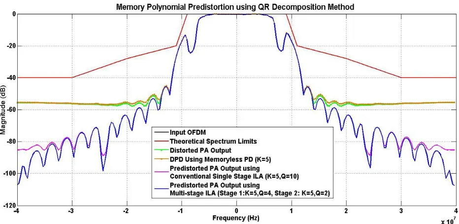
Figure 5.1 and 5.2 shows the spectral regrowth suppression capabilities of single stage memory polynomial PD and multi stage polynomial PD respectively. As observed from the plot, the memory polynomial predistortion can attain achieve sufficient amount of spectral regrowth suppression with single stage or with multi stage. Also it can be inferred from plots that for a PA with memory a memory less predistorter can attain only limited performance as compared with the performance of a memory polynomial predistorter.

(7)

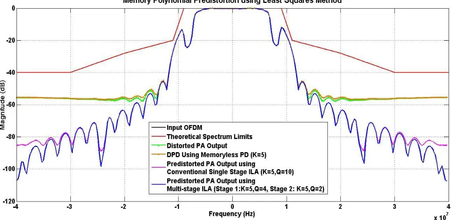
Figure 5.2 Spectrum plot of memory polynomial predistortion using Least Squares.

From the spectrum plots it can be inferred that the spectral regrowth capabilities of the two stage ILA approach is higher than that of conventional single stage approach. The two stage approach can almost suppress all the spectral broadening with less complexity.

VI.CONCLUSION

In this paper we proposed a multi-stage indirect learning architecture (ILA) with low identification complexity. The multi-stage ILA, PD is implemented in two or more stages. The reference PA model used for simulation is Wiener-Hammerstein model. The spectral regrowth suppression capability is considered for analysing the performance of the two approaches. It was shown that this multi-stage ILA was able to achieve same or even better performance than the conventional ILA but with significantly lower identification complexity.

REFERENCES

[1] S. C. Cripps. “RF Power Amplifiers for Wireless Communications,” Artech House, Inc., Norwood, MA, USA, 2006.

[2] T. S. Rappaport. “Wireless Communications: Principles and Practice,” (2nd Edition). Prentice Hall PTR, December 2001.

[3] R. Raich and G. T. Zhou, “On the modelling of memory nonlinear effects of power amplifiers for communication applications,” in Proc. IEEE Digital Signal Processing Workshop, Oct. 2002.

[4] H. S. Black, “Inventing the negative feedback amplifier," IEEE Spectrum, vol. 14, pp. 55-60, Dec. 1977

[5] F. Perez, E. Ballesteros and J. Perez, “Linearization of microwave power amplifiers using active feedback networks,” IEEE Electronics Letters, vol. 21, no. 1, pp. 9-10, Jan. 1985.

[6] L. Ding, et al., "A robust digital baseband predistorter constructed using memory polynomials," IEEE Transactions on Communications, vol.52, no.1, pp. 159-165, Jan. 2004.

[7] C. Eun and E. J. Powers, “A new Volterra predistorter based on the indirect learning architecture,” IEEE Trans. Signal Processing, vol. 45, pp. 223– 227, Jan. 1997.

[8] P. Crama and J. Schouken, “Wiener-Hammerstein system estimator initialization using a random multisine excitation,” 58th ARFTG Conf. Dig., Dec. 2001.

(8)

[10] Z. Ma, M. Zierdt, and J. Pastalan, “Characterization of power amplifier memory effect for digital baseband predistortion.” unpublished work, Jan. 2001

[11] Lei Ding and G. Tong Zhou. “Effects of Even-Order Nonlinear Terms on Power Amplifier Modelling.” IEEE Transactions On Vehicular Technology, Vol. 53, No. 1, January 2004