Fragility analysis methods: Review of existing approaches and application

(1)

Fragility analysis methods: Review of existing approaches and application

Max Gündel1, Irmela Zentner2

1_{Seismic Engineer, Wölfel Beratende Ingenieure, Germany}

2_{R&D Engineer, EDF R&D AMA Analyses Mécaniques et Acoustique, France}

ABSTRACT

In seismic reliability analysis the total failure probability is determined by combining the fragility curve - representing the response of the structure to seismic excitation - with the seismic hazard curve. The determination of fragility curves has a long tradition in the nuclear industry and reaches back to the 1970s. Since the late 1990s also for ordinary buildings seismic reliability analysis became more important and formed the bases for the development of new seismic standards. Several methods are available to build fragility curves relying on different assumptions and restrictions, level of detail and type of failure modes under consideration.

In this paper, different fragility analysis methods are described and their advantages and disadvantages are discussed: (i) the safety factor method, in which the fragility curve is estimated on an existing deterministic quasi-static design; the numerical simulation method, in which the parameters of the fragility curve are obtained by (ii) regression analysis or (iii) maximum likelihood estimation from a set of nonlinear time history analysis at different seismic levels; (iv) the incremental dynamic analysis which is based on numerical simulation and the scaling of accelerograms until failure. These four fragility analysis methods are applied to determine fragility curves for the 3-storey reinforced concrete shear wall building of the SMART2013 benchmark project. Advantages and disadvantages of the methods are illustrated and the impact of the simplifying assumptions (e.g. lognormal curves, scaling) are accessed.

INTRODUCTION

Seismic reliability analysis

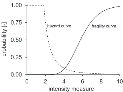
In seismic reliability analysis the structural response is investigated separately from the seismic hazard. The structural response is described by the fragility curve Pf(a) (cumulative distribution function of

capacity) and the hazard by the seismic hazard curve H(a)=k0·a-k both as a function of the seismic

intensity a, Figure 1. Multiplication of fragility curve and hazard curve as well as integration over the seismic intensity leads to the total failure probability Pf,totalof a structure for a given reference period.

( )

ò

¥

× -=

0

, h a P a da

P_f _total _f

(1)

(2)

23rd Conference on Structural Mechanics in Reactor Technology Manchester, United Kingdom - August 10-14, 2015 Division VII

Figure 1. Hazard and fragility curves.

Definition of fragility curve

The fragility curve is the conditional failure probability of a structure, element or component given the seismic intensity. Failure is not necessarily the collapse of the structure but can be described by any threshold value for relevant structural parameters. According to the latter definition, failure occurs when the demand exceeds a defined limit capacity. The fragility curve is usually approximated by a lognormal distribution function, Figure 1 with median Am and lognormal standard deviation b:

÷÷

ø

ö

çç

è

æ

-F

=

b

m f

A

a

P

ln

(2)

Overview of fragility analysis methods

A number of methods are available to build fragility curves, which differ from each other regarding assumptions, restrictions, the level of detail and type of failure modes under consideration.

The scaling method is widely used in nuclear industry practice. The development of the method goes back to the late 1970s and was considerable influenced by Cornell, Kennedy and Ravindra (Kennedy, et al., 1980), (Kennedy, et al., 1984). Starting from an existing deterministic design several sources of conservatism and uncertainties are accessed and considered to determine the mean capacity and its scattering of the structure. The method can be carried out with analytical calculations and do not need time-consuming numerical simulations.

The numerical simulation method was developed nearly in parallel to the scaling method; however, due to its high computational costs the application in practice is limited. A number of time history analyses are carried out using a set of seismic records characteristic for the site as well as a set of random input parameters representative for the main structural properties. The set of simulations is evaluated with respect to a suitable damage indicator (e.g. inter-storey drift) to estimate the mean capacity and scattering of the structure.

The use of incremental dynamic analysis to build fragility curves is more often applied for ordinary building structures and is rather unusual in nuclear industry. The development of this method is closely connected with the work of Cornell (Cornell, et al., 2002) in the 1990s and formed the probabilistic basis of the new deterministic seismic design concept for steel structures in FEMA350. For a set of seismic records a number of time history analyses are carried out, where each record is scaled up until the collapse of the building (i.e. dynamic instability) occur. The fragility curve is estimated on the basis of the fraction of collapses at each seismic level.

Furthermore, pushover analyses (Gündel, et al., 2014) or experimental tests can be used to estimate fragility curves; however, these are not considered in this study.

0.00 0.25 0.50 0.75 1.00

0 2 4 6 8 10

pr

ob

ab

ili

lty

[

-]

intensity measure

(3)

DESCRIPTION OF CASE STUDY

Structure and Numerical model

The fragility analysis methods were applied on a trapezoidal, three-storey reinforced concrete structure, which was design, built and analysed experimentally and numerically within the SMART2013 international benchmark project (Figure 2, left). The structure was a 1:4 scaled mock-up representing a simplified half part of a nuclear electrical building. The dimensions were 3.10 x 2.55 m in plan and the height was 3.65 m. Torsional effects were activated by significant irregularities in plan. To obtain accelerations and stresses similar to the real structure additional masses were fixed on each floor. The total seismic mass was about 45.7 t. The structure was made of concrete strength C30/37 and reinforcement Bst500. The mock-up was anchored at a shaking table; however, in the fragility analysis a numerical model was used, in which the shaking table was replaced by equivalent foundation impedances. The mock-up was designed according to the French nuclear regulation RFS V.2 G and current ASN Guidelines (Richard, et al., 2014). The design spectrum has a peak ground acceleration of 0.2 g and corresponds to a magnitude 5.5 earthquake at a distance of 10 km and (Figure 3, left). The lateral load resisting systems is provided by shear walls with minor and major openings and a thickness of 0.1 m. The main eigenmodes and frequencies (of the numerical model with equivalent foundation impedances) are rocking in x- and y-direction at 5.97 Hz and 5.38 Hz, translation in z-direction at 14.56 Hz and torsion at 15.94 Hz.

Figure 2. Mock-up of SMART2013 benchmark project (Richard, et al., 2014) (left) and its numerical model (right).

The numerical model was built with Abaqus 6.13 (Dassault Systemes, 2014). Walls, floors and downstand beams were modelled by shell elements, the foundation was built by solid elements and for the columns beam elements were used. Foundation impedances were included by connecting the lower surface of the foundation rigidly to a master node, which was supported by translational and rotational springs and dashpot elements. As material model, the concrete damage plasticity model for concrete and the Johnson-Cook model for reinforcement were applied. The material model parameters were chosen as characteristic values given in Eurocode 2 or determined acc. to Model Code 1990 (Rowe, et al., 1993). For the numerical simulation of fragility curves, uncertainty on following model parameters was considered, at which lognormal distribution were supposed (Richard, et al., 2014):

- concrete tensile strength of floor 1, 2 and 3 (mean value = 3 N/mm², COV = 33 %), - foundation stiffness (COV = 1 %) and damping (COV = 2 %),

(4)

where COV designs the coefficient of variation. All random variables were supposed to be uncorrelated excepting the foundation stiffness, which has a coefficient of 0.80. The uncertainty on other material or geometrical parameters as well as on the threshold of the damage criteria was not accounted for.

The maximum Inter-Storey Drift (ISD) was considered as continuous damage indicators, with thresholds of 1% associated with extended damage (Richard, et al., 2014) respectively life safety (FEMA356) and of 2 % associated with collapse (FEMA356). The latter threshold was chosen for comparison the numerical methods with the safety factor method.

Seismic input and seismic indicators

In the numerical simulation method and in the incremental dynamic analysis method sets of synthetic generated horizontal accelerograms were used (Zentner, et al., 2014). 50 pairs of correlated accelerograms were generated with Code_Aster to be compatible with median and +/- 1s spectra. The target spectrum is related to a magnitude 6.5 earthquake at a distance of 9 km, which was chosen to obtain time histories that are likely to damage the structure. Such a scenario is not representative of any French or German site where the seismic hazard level is much lower. The response spectra are shown in Figure 3, right.

The characteristics of accelerograms can be described by different seismic motion indicators. The choice of the indicator has an influence on the scattering of the fragility curve; i.e. suitable chosen indicators can reduce the inherent introduced uncertainties of the seismic action into the fragility curve. However, the effectiveness of the seismic indicator strongly depends on the type of structure and the controlling failure mechanism. The seismic indicators considered in this case study are defined as follows:

- Peak ground acceleration (PGA):

[

t tf

]

a

( )

t t 0,

max

Î

- Pseudo-spectral acceleration (PSA) : S_a(f₀)

- Average Spectral Acceleration (ASA):

_ò

(

_-

)

0

6 . 0

0 0 0.6

) ( f

f

a f df f f

S

were f0 is the fundamental eigenfrequency of the structure. While PGA are only related to the seismic

ground motion, PSA and ASA depend on the dynamic behaviour of the structure. In the numerical analysis, the structure is submitted to 2D horizontal seismic load. This is accounted for by considering the max and the geometric mean (mean in log-space) of the two horizontal indicator values.

Figure 3. Design spectrum for D = 5% (left) and spectra of simulated accelerograms (right). 0.01

0.10 1.00 10.00

0.1 1.0 10.0 100.0

PSA

[g

]

frequency [1/s]

0.01 0.10 1.00 10.00

0.1 1.0 10.0 100.0

PSA

[g

]

frequency [1/s]

median+s median

(5)

SAFETY FACTOR METHOD

Methodology

The starting point of the safety factor method is an existing deterministic seismic design of the structure. On this basis several sources of conservatisms (and unconservatisms) are accessed to estimate a realistic median capacity of the structure. Additionally, uncertainties of each source are assessed to obtain the overall randomness of the capacity. Finally, the capacity of the structure, characterized by the associated peak ground acceleration, is described by the median value ܣ_௠ as well as two lognormal distributed random variables with a median of 1. The random variables represent the total epistemic uncertainty eU

and the total aleatory uncertainty eR.

U R m

A

A= ×

e

×

e

(3)

ܣ௠ represents the best estimate of the actual capacity and is determined by the product of the safe

shutdown earthquake ASSE from the deterministic analysis and the median value of the safety factor F. F is

the product of a number of factors and can be described by following formula (Kennedy, et al., 1980):

RS

S

F

=

×

m

×

(4)

where FS is the strength factor (considering e.g. mean to characteristic material strength, safety factors),

Fm is the dissipation factor (i.e. similar to coefficient R in IBC or q in Eurocode 8) and FRS is the structural

response factor. The latter one can be subdivided in following components:

SS EC MC M SA

RS

F

=

×

_d

×

(5)

where FSA is the spectral shape factor; Fdis the damping factor; FM is the modelling factor; FMC and FEC

are factors for the combination scheme of modal parts respectively horizontal components of the seismic action; FSS is the factor for soil-structure-interaction. For each factor the median value and the epistemic

and aleatory uncertainties has to be estimated. Procedures and indicative values for this purpose can be found in (EPRI, 1994). It is assumed that each source of randomness is lognormal distributed so that the product of all factors is again lognormal distributed and the lognormal standard deviation bR (aleatory)

and bU (epistemic) is the square root of the sum of the squares. The fragility curve is written as follows:

( )

(

)

( )

_÷÷

ø ö ç

ç è

æ ₊ _×_F

F =

-R U m f

Q A

a a

P

b

1

/ ln

(6)

Besides the median fragility curve, where the epistemic uncertainties are zero (i.e. F-1(Q) = 0), fragility curves for any confidence interval can be calculated (e.g. F-1(Q) = -1.65 for 95 %).

Application and results

The SMART2013 benchmark structure was designed according to current nuclear codes for a peak ground acceleration of 0.2 g. (Richard, et al., 2014). Median values and lognormal standard deviations of all factors required to build the fragility curve were determined in line with (EPRI, 1994), Figure 4 left. The strength factor FS was determined by comparing the shear or by bending capacity of each shear wall

with the internal forces obtained in the seismic load combination. The median capacities were determined by formulas provided in (EPRI, 1994) with mean values for yield strength of the reinforcement and concrete strength. The influence of material strength scattering was considered within the aleatory uncertainty, while the epistemic uncertainties were estimated in line with (EPRI, 1994). The governing structural element is the short wall in x-direction under bending. The median value of the dissipation factor Fm was determined as a function of the exploited ductility ratio. The ductility ratio was assumed to

(6)

epistemic uncertainties was determined as a function of the ductility ratio (EPRI, 1994). The median values for all sub-factors required for the structural response factor were chosen to 1.0; it was assumed that the design of the structure is carried out with methods according to the state of the art without significant conservatisms. However, scattering from several sources were considered (e.g. determination of eigenfrequencies, numerical model, soil structure interaction).

The safety factor was obtained as product of FS, Fm and FRS to 6.60, so that the median capacity of the

structure resulted to Am = 13.21 m/s². The aleatory uncertainties lead to a lognormal standard deviation of bR = 0.28, where the main source of randomness was the spectral shape factor. The epistemic

uncertainties were significant higher and lead to a lognormal standard deviation of bU = 0.47. The main

sources of randomness were the strength factor, spectral shape factor and model factor.

Factor Median value

Scattering (aleatory)

Scattering (epistemic)

ܺ෨ bR bU

F 6.60 0.28 0.47

FS 2.74 0.04 0.22

Fm 2.41 0.04 0.14

FRS 1.00 0.27 0.39

FSA 1.00 0.20 0.24

Fd 1.00 0.00 0.00

FM 1.00 0.00 0.25

FMC 1.00 0.15 0.00

FEC 1.00 0.11 0.11

FSS 1.00 0.02 0.13

Figure 4. Median value and lognormal standard deviation for epistemic as well as aleatory uncertainties (left) and fragility curves (right) based on the scaling method (bending failure of shear wall in x-direction)

NUMERICAL SIMULATION USING LINEAR REGRESSION IN LOG SPACE

Methodology

This methodology is based on nonlinear time history analysis in order to obtain a data sample that can be used for the evaluation of (lognormal) fragility curves. For this purpose, the seismic load is characterized by N ground motion histories in agreement with the site-specific hazard (Zentner, et al., 2011). In general Latin hypercube sampling is used to propagate uncertainty in addition to random seismic excitation. The method assume that a sample of N input-output (ai, yi), i = 1,...N, pairs is available. The input is the

ground motion indicator (seismic intensity level ai) and the output variable yi is the continuous damage

measure. The continuous damage measure Y is modelled as lognormal random variable:

h

a

c

b

Y

=

(7)

where h is a lognormal random variable with a median of 1 and a logarithmic standard deviation s . It is supposed that the structure fails or reaches a certain damage level when the variable Y exceeds a threshold

Ycrit such that Pf(a) = P(Y > Ycrit|a)

. The parameters

b, c and scan be conveniently determined by linear

regression:

ε,

+ ) ( c + b =

(Y) ln( ) ln a

ln

(8)

where e = log(h) is a normal random variable and beta is obtained as the standard deviation of the regression error. Moreover, defining Ycrit = b∙acritc we have

0.00 0.25 0.50 0.75 1.00

0 10 20 30

pr

ob

ab

ili

ty

[

-]

PGA [m/s²]

0.5 non-exceedence probability 0.05 and 0.95

non-exceedence probability

composite curve

(7)

úû ù êë é c /b) (Y = A crit m ln

exp

.

₍₉₎

In consequence, the fragility curve is described by a lognormal distribution with a median equal to the seismic capacity Am and the lognormal standard deviation b = s/c:

÷ ø ö ç è æ = ÷ ø ö ç è æ c ) /A ( Φ ) /A ( c )=Φ (

P_f m m

/ ln ln s a s a a

(10)

One major advantage of the linear regression approach is that it can be used even in cases when no failure is observed. It does not require scaling of accelerograms and is quite robust even for small sample sizes.

With the numerical model of the SMART2013 benchmark structure N = 50 time history analyses were carried out. In each run one pair of accelerograms in combination with one set of parameters for uncertain structural properties were used. The damage measure is the maxISD and the seismic indicators are the maximum and geometric mean of the PGAs and the PSAs as well as the maximum ASA (see section

‘Description of the case study_’. Each run was evaluated in terms of damage indicators and seismic indicators to obtain an input-output data sample. For each input-output data sample the median capacity

Am and the lognormal standard deviation b were determined by linear regression using Code_Aster. The

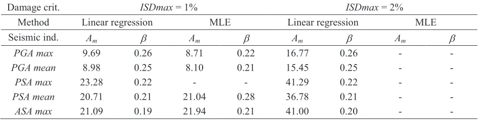
results are summarized in Table1.

Figure 5. Determination of fragility curves by linear regression (damage indicator: ISDmax, damage threshod 1 %).

Table 1: Fragility curve parameters obtained with numerical simulation method using Linear regression and MLE.

Damage crit. ISDmax = 1% ISDmax = 2%

Method Linear regression MLE Linear regression MLE

Seismic ind. Am b Am b Am b Am b

PGA max 9.69 0.26 8.71 0.22 16.77 0.26 - -

PGA mean 8.98 0.25 8.10 0.21 15.45 0.25 - -

PSA max 23.28 0.22 - - 41.29 0.22 - -

PSA mean 20.71 0.21 21.04 0.28 36.78 0.21 - -

ASA max 21.09 0.19 21.94 0.21 41.00 0.20 - -

0.00 0.01 0.02 0.03 0.04

0 10 20 30

ISD

max

[m]

PGAmax[m/s²] Am,1 fitted power law function Ycrit,1 observations Am,2 Ycrit,2 0.00 0.25 0.50 0.75 1.00

0 10 20 30

pr ob ab ili ty [ -]

PGAmax[m/s²] Am

Linear regression MLE

(8)

23rd Conference on Structural Mechanics in Reactor Technology Manchester, United Kingdom - August 10-14, 2015 Division VII NUMERICAL SIMULATION USING MAXIMUM LIKELIHOOD ESTIMATION

Methodology

As for linear regression, the method starts from a sample of N input-output (ai, xi), i = 1,...N, pairs. The

maximum likelihood method however assumes a binary damage measure: xi =1 if damage occurs and 0

otherwise. If the damage measure is continuous, it has to be transformed into binary data according to the failure criterion. The two parameters Am and b are obtained by maximizing the likelihood function L, so

that the most plausible parameter values, given the fragility model and the data, are chosen:

[

] [

i

]

xi

i f x i f N

i

P

a

P

a

L

-=

-P

=

1

(

)

1 (

)

[

]

)

ln(

min

arg

)

,

(

,

L

A

m

A e

m

e

₌

-b

b

(11)

where Pf is as in expression (2). The maximum likelihood estimator allows to determine the most

plausible fragility curve given the discrete data (results from numerical simulation).

For the Maximum Likelihood Estimation the same input-output pairs as for the Linear regression analyses were used. The results obtained for ISDmax = 1% (extended damage) using Code_Aster are shown in Table 3. The MLE method could not be used for the collapse threshold (ISDmax = 2%), as, obviously, the optimization algorithm cannot converge if no failure is observed.

NUMERICAL SIMULATION USING INCREMENTAL DYNAMIC ANALYSIS

Methodology

Incremental dynamic analyses (IDA) are used to obtain fragility curves for building structures associated with their actual collapse. IDAs are performed by means of a number of nonlinear time history analyses with repeatedly scaling an accelerogram until the accelerogram causes collapse of the structure. Often the

PSA is used as scaling factor and scaling with a factor of up to 30 do not introduce significant bias or additional scattering (Pinto, et al., 2004). Uncertainties of the structure are considered by using one set of uncertain parameters in each IDA, which influences the dynamic response and the capacity of the structure.

Using this method each accelerogram has a single intensity measure associated with collapse. By repeating this procedure for a set of N accelerograms, one obtains a set of seismic intensities associated with the onset of collapse. The probability of collapse at a given intensity level a can then be estimated as the fraction of records for which collapse occurs at a level lower than a (Equation 2). These discrete failure probabilities are the empirical fragility curve of the structure. For an analytical description of the fragility curve, e.g. by a lognormal distribution, Linear regression (Porter, et al., 2007) or MLE can be used (Baker, 2011). In opposite to the aforementioned numerical simulation methods the statistical analysis methods in the IDA are used to fit directly the fragility curve to the discrete results.

IDAs with 7 pairs of accelerograms, chosen from the set of 50 accelerograms described before, were carried out using the numerical model of the benchmark structure. The records were scaled up to a PGA

of 34 m/s² with a step size of 2 m/s²; in total 119 time history analyses were carried out. For each suite of IDA another set of uncertain parameters is used. In Figure 6, the roof drifts in x-direction over the PGA

(9)

The IDA was stopped if the time history analysis did not converge and dynamic instability of the structure occurs. This intensity level corresponded to collapse of the structure and was reached for PGAs between 14 m/s² and more than 34 m/s². However, the scattering was very high and rather due to numerical problems than mechanical behaviour. This is why the IDA in conjunction with a failure threshold is preferred. For this reason and to compare the results with the other numerical methods, ISDmax with thresholds of 1% and 2% were evaluated to build the fragility curve. The latter threshold was close to the instability of the structure. Furthermore, the maximum and geometric mean of PGA and PSA were considered as seismic indicator. To fit lognormal distribution to the empirical fragility curve Linear Regression and Maximum Likelihood estimation were used for the 7 seven data points, Table 2.

Figure 6. Incremental dynamic analysis with collapse frequency (left); empirical and fitted fragility curve (damage indicator: ISDmax, damage threshod 1 %) (right)

Table 2: Fragility curve parameters obtained obtained with IDA method.

Damage crit. ISDmax = 1% ISDmax = 2 %

Method IDA Linear regr. IDA MLE IDA Linear regr. IDA MLE

Seismic ind. Am b Am b Am b Am b

PGA max 9.91 0.22 10.03 0.21 13.65 0.23 13.87 0.24

PGA mean 9.52 0.18 9.67 0.18 13.13 0.24 13.31 0.25

PSA max 20.69 0.19 20.97 0.20 29.91 0.27 30.01 0.26

PSA mean 19.82 0.22 20.04 0.20 28.32 0.30 28.57 0.27

SUMMARY AND DISCUSSION

In this paper four fragility analysis procedures, namely the Safety Factor method, the Numerical simulation in conjunction with linear Regression, the Numerical simulation in conjunction with the maximum likelihood estimator (MLE) and the Incremental dynamic analysis method (IDA) were applied to determine fragility curves for a 3 storey reinforced concrete structure. These methods have advantages and disadvantages and their use has to be adapted to the type of data and computational resources available.

The Safety Factor method is a simple and efficient analytical fragility analysis procedure, which requires, though, a number of assumptions based on experience. Both the IDA and the Safety Factor Method are based on scaling of ground motion. The IDA performs the scaling in the time domain to allow for nonlinear structural analysis. IDA analysis allows directly the assessment of collapse of the structure;

0.00 0.05 0.10 0.15 0.20

0 10 20 30

maxi

mum roo

f drift X

[m]

PGAmax[m/s²] roof drift 2 %

0.00 0.25 0.50 0.75 1.00

0 10 20 30

pr

ob

ab

ili

ty

[

-]

PGAmax[m/s²] fitted fragility curve by MLE

discrete values

(10)

however, this is at the cost of a number of time consuming nonlinear analyses near collapse (109 vs. 50 for the other simulation methods).

Both, the Simulation Method with MLE and the IDA method can be used in conjunction with other probability distribution than lognormal while the linear regression method is linked to the hypothesis of a lognormally distributed damage measure. Nevertheless, in opposite to the other methods, the linear regression approach can be used even in cases when no failure is observed, is quite robust even for small sample sizes and the log-standard deviation does not depend on the failure threshold.

The main conclusions of the applications to the 3 storey reinforced concrete structure can be summarized as follow:

- The median capacity of the fragility curves at a threshold of maxISD = 1% is close for all simulation methods. At a threshold of maxISD = 2% the IDA leads to smaller values; however, 7 sets of accelerograms for IDA might be too few to propagate uncertainty in the framework of Monte Carlo simulation.

- The lognormal standard deviation of the fragility curves at a threshold of maxISD = 1% is rather smaller for IDA in respect to the Regression method and at maxISD = 2% rather higher.

- The differences between the performances of the damage indicator under consideration are minor. - The 2% maxISD threshold correlates well with onset of collapse identified in the IDA.

- The median capacity of the fragility curves obtained by the Safety Factor method correlates well with the other methods using a threshold maxISD = 2%. The lognormal standard deviation of the fragility curves in the Safety Factor method, which corresponds to the aleatory scattering, is similar to the scattering from the other methods. However, additional epistemic uncertainties are accounted for in the Safety Factor method.

Confidence intervals should be evaluated for the simulation-based methods including IDA, in order to further evaluate and compare the performance of the different approaches.

REFERENCES

Baker, J. W. 2011. Fitting Fragility Functions to Structural Analysis Data Using Maximum Likelihood Estimation. 2011.

Code_Aster. R4.05.05 Génération de signaux sismiques and U2.08.05 Propagation des incertitudes et calcul de courbes de fragilité.

Cornell, C. Allin, et al. 2002. Probabilistic Basis for 2000 SAC Federal Emergency Management Agency Steel Moment Frame Guidelines. Journal of Structural Engineering. 2002, Bd. 128, 4, S. 526-533.

Dassault Systemes. 2014. Abaqus User Manual. 2014.

EPRI. 1994. Methodology for Developing Seismic Fragilities. s.l. : Electrical Power Research Institute, 1994. Gündel, Max and Hoffmeister, Benno. 2014. Stochastic seismic load model for push-over analyses. [book auth.] A. Cunha, et al. Proceedings of Eurodyn 2014. Porto : s.n., 2014.

Kennedy, R.P. and Ravindra, M.K. 1984. Seismic fragilities for nuclear power plant risk studies. Nuclear

Engineering and Design. 1984, Vol. 79, pp. 47-68.

Kennedy, R.P., et al. 1980. Probabilistic seismic safety study of an existing nuclear power plant. Nuclear

Engineering and Design. 1980, Vol. 59, pp. 315-338.

Pinto, P.E., Giannini, R. and Franchin, P. 2004. Seismic Reliability Analysis of Structures. Pavia : IUSS Press, 2004. Porter, K., Kennedy, R. and Bachman, R. 2007. Creating Fragility Functions for Performance-Based Earthquake Engineering. Earthquake Spectra. 2007, Vol. 23, 2, pp. 471-489.

Richard, Benjamin and Chaudat, Thierry. 2014. Presentation of the SMART2013 International Benchmark. 2014. SEMT/EMSI/ST/12-017 H.

Rowe, Roy E. and Walther, René. 1993. CEB-FIP Model Code 90. London : Thomas Telford, 1993.

Zentner, I., et al. 2011. Numerical methods for seismic fragility analysis of structures and components in nuclear industry - Application to a reactor coolant system. Georisk. 2011, Vol. 2, 5, pp. 99-109.

Zentner, Irmela, et al. 2014. Generation of spectrum compatible ground motion and its use in regulatory and performance based seismic analysis. [book auth.] A. Cunha, et al. Proceedings of the 9th International Conference