Division VII
METHOD FOR DETECTING OPTIMAL SEISMIC INTENSITY INDEX
UTILIZED FOR GROUND MOTION GENERATION IN SEISMIC PRA
Sayaka Igarashi1, Shigehiro Sakamoto2, Tekeshi Ugata3, Akemi Nishida4, Ken Muramatsu5, and Tsuyoshi Takada6
1 Research Engineer, Technology Center, Taisei Corporation, Japan
2 Executive Chief Research Engineer, Technology Center, Taisei Corporation, Japan
3 General Manager, Nuclear Facilities Division, Taisei Corporation, Japan
4 Principal Researcher, Japan Atomic Energy Agency, Japan
5 Visiting Researcher, Japan Atomic Energy Agency, Japan
6 Professor, Department of Architecture, The University of Tokyo, Japan
ABSTRACT
For the purpose of improving the precision of probabilistic seismic risk assessment (seismic PRA) for Nuclear Power Plants (NPPs), Nishida et al. (2013, 2016) developed the methodology for generating hazard-consistent ground motions (HCGMs) based on stochastic fault models which include seismic-source uncertainties by Monte Carlo Simulation. The authors also demonstrated the advantage of the PRA method based on HCGMs by examining the differences between the damage probabilities of equipment system due to HCGMs and those due to other ground motions sets (Igarashi et al., 2015). On the other hand, seismic PRA with HCGMs would require a lot of computer power. The optimization of ground-motions generations is one of the most important subjects for practical applications of this PRA method.
For efficient ground-motions generations, seismic sources for the ground-motion generations should be selected effectively, and this can be achieved by utilizing optimal seismic intensity index in the hazard analysis. In this study, the method for detecting the optimal seismic intensity index which corresponds with damage probabilities of the target equipment system is developed. This method is based on the examination of the discrepancies of generated ground-motions order which are sorted by the damage probabilities of the system or by their seismic intensity indices.
In order to validate the method, the optimal index detections were attempted for some cases of an equipment system, which has different weak equipment component depending on the cases. As a result, the smallest discrepancy was obtained with the expected seismic intensity index for each case, and the validity of the proposed method was confirmed.
INTRODUCTION
In preceding studies by Nishida et al.(2013, 2016), a next-generation methodology of seismic PRA has been developed for the purpose of improving the precision and the reliability of probabilistic seismic risk assessment (seismic PRA) of Nuclear Power Plans (NPPs). The proposed seismic PRA is conducted based on time-history response analyses utilizing a lot of ground motions simulated with stochastic fault models, where their stochastic characteristics are simulated by Monte Carlo simulations (MCS). Seismic sources where stochastic faults are settled are selected according to the contribution to the hazard at the target site, however, there still remain a lot of seismic sources that should be taken into account. In order to conduct such seismic PRA, a large computer power would be required, especially to generate ground motions. Some efficient evaluation methods for generating ground motions should be adopted for the practical applications of the next-generation seismic PRA.
facilities where systems with arbitrary response characteristics is installed. The proposed method enables us the effective selection of seismic sources which contribute the seismic risk (for instance, a building functional loss due to the damages of components in the system), therefore, the reduction of the sampling number of generated ground motions would be expected. The advanced seismic PRA utilizing ground motions simulated with fault models can be conducted more effectively.
EFFICIENT METHOD FOR SEISMIC PRA UTILIZING GROUND MOTIONS WITH FAULT MODELS
The seismic PRA methodology by Nishida et al. (2013, 2016) is the time-history-analysis based risk assessment scheme. The ground motions input for the seismic PRA are generated with a lot of fault models. The fault models are settled on seismic sources which contribute to the hazard at the target site so as to include the uncertainties of seismic-source characteristics by MCS. The ground-motion time histories are evaluated based on the ground motion generation method such as a stochastic Green’s function method. The distinct advantage of the proposed methodology is that the seismic risk can be continuously evaluated without eliminating rich information of ground motions. Another advantage is that complicated behaviours of non-liner structural response can be calculated by dynamic response analyses and they are included into the result of risk assessment. Therefore, the advanced method utilizing ground motions with fault models can be expected for the more realistic and reliable seismic PRA.
On the other hand, there are some issues about utilizing the ground motions with fault models for seismic PRA. For example, a lot of ground motions are required because they should represent the seismic hazard of the target site. In the study of Nishida et al. (2013, 2016), the ground motions were generated from several seismic sources which contribute to the hazard of a maximum acceleration on the free rock surface. It is because they are attempt to be utilized for the risk evaluation of an NPP facility, which has nuclear equipment systems whose damages correlate with short-period seismic intensity. In the case where damages do not correlate with short-period seismic intensity, another intensity that correlate well with damages should be found for the appropriate hazard analysis and for the effective seismic source selection. In this study, an efficient method for detecting an optimal seismic intensity in order to generate ground motions from risk-contributed seismic sources.
Seismic intensity Frequency
10-5
y
Seismic source
Target site
x
【Efficient evaluation method】
Damage probability evaluation of equipment system
1. Seismic hazard analysis
Seismic sources selection
2. Settlement of fault models in seismic sources
Fault models with stochastic characteristics
Ground motions generation
Ground motions consistent with hazard based on the intensity y 3. Extraction of ground motions
5. Evaluation of building functional loss
Tank Tank P omp
P ipe P ipe P ipe P ipe Tank
Equipment system
4. Time history response analysis Ground motions
Reconsideration of optimal seismic intensity index for building functional loss
Structural model
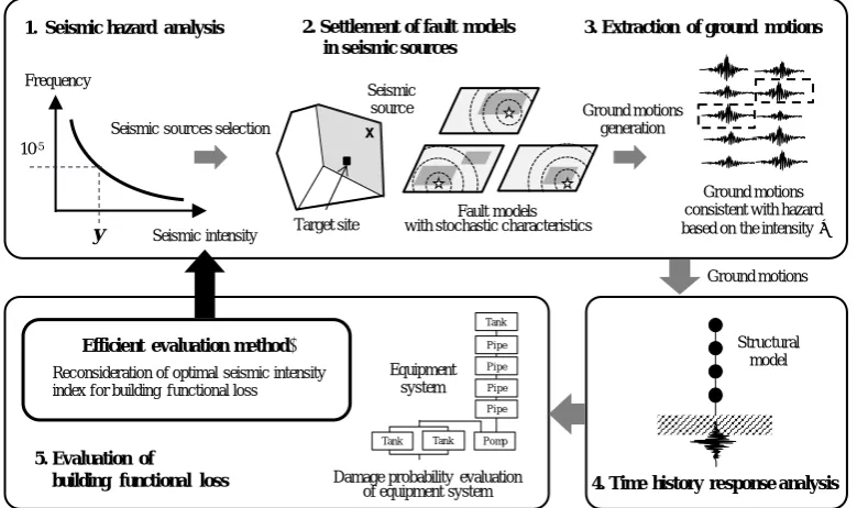
Figure 1 shows the schematic diagram of seismic PRA adopting the proposed efficient method. Firstly, the seismic hazard analysis is conducted to clarify the hazard contributions of seismic sources around the target site. At this step, the seismic intensity index for the hazard analysis can be the commonly used one such as the maximum acceleration. The ground motions are generated with fault models of seismic sources which show a high contribution to the seismic hazard, so as to incorporate the uncertainties of seismic-source characteristics by MCS. Then, intensity indices of generated ground motions are evaluated as well as the risk such as a building functional loss due to them. Evaluated indices are compared with each other for detecting the optimal index that correspond with the risk.
If the detected index is not the same index that was used for the previous hazard analysis, hazard analysis and ground motion generation should be conducted again with the detected index. If the detected index is the one for the previous hazard analysis, the detected index can be settled as the optimal index. Once the optimal index is settled as a seismic intensity index for seismic hazard evaluation, the seismic sources which contribute to seismic risk can be obtained effectively, and the ground motions focused on the seismic risk can be generated.
METHOD FOR DETECTING OPTIMAL SEISMIC INDEX
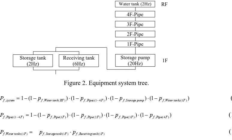
In this chapter, the method of detecting an optimal seismic intensity index, which has the best correlation with the seismic risk of target facility, will be proposed. Here, the “seismic risk” is defined as a building functional loss due to the seismic damage of system in Figure 2. The equipment system assumes a water supply system, the same system with that in the study by Igarashi et al.(2015). It consists of some equipment components such as water tanks, pumps and pipes. The damage probability of the entire system was evaluated based on the fault tree analyses. Concretely, the damage probability of
equipment system in Figure 2 Pf,system was calculated by Eqs.(1)~(1-2).
Figure 2. Equipment system tree.
) 1
( ) 1
( ) 1
( ) 1
(
1 , ( ) , (1~4 ) , , (1 )
,system fWatertankRF f Pipes F fStoragepump fWatertanks F
f p p p p
P (1)
) 1
( ) 1
( ) 1
( ) 1
(
1 , (1 ) , (2 ) , (3 ) , (4 )
) 4 ~ 1 (
,Pipes F fPipe F fPipe F fPipe F f Pipe F
f p p p p
P (1-1)
) 1 ( ,
) 1 ( , ) 1 (
,Watertanks F f Storagetank F fReceivingtank F
f p p
P (1-2)
The proposed method intends to detect the most appropriate seismic intensity index for hazard analysis in seismic PRA. The optimal index is selected from some candidate indices calculated with ground-motion time history. The selected index is the optimal one that can represent the building functional loss the most properly, in other words, the selected index has the best correlation with the seismic damage of equipment system.
RF
1F 4F-Pipe
3F-Pipe
2F-Pipe
1F-Pipe
Storage pump (20Hz) Storage tank
(2Hz)
Receiving tank (6Hz)
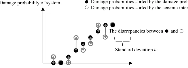
Figure 3 shows a schematic drawing of the proposed method for detecting seismic intensity index which correlate with the building functional loss. The plots in Figure 3 shows the distribution of damage probabilities by each ground motion. The black plots show the damage probabilities of the system arranged in the order of themselves, that is to say, the distribution shows the correct order of damage probabilities by ground motions with fault models. On the other hand, the grey plots show the damage probabilities arranged in the order of a seismic intensity calculated from ground-motion time histories. The volume of discrepancies between the black ones and the grey ones indicates the degree of correlation between the damage probability of equipment system and the seismic intensity. Therefore, if a seismic intensity index shows the smallest discrepancies of all candidate indices, it might have the best correlation
with the seismic risk. In this study, the volume of discrepancies of each seismic intensity index i is
compared by evaluating a standard deviation i calculated from Eq.(2), and then the index which has the
smallest i is detected as an optimal seismic intensity of all candidate indices.
Figure 3. Schematic drawing of proposed method for detecting an optimal index.
1
)
( 2
) (
| , .) (
| ,
N P P
N
i index Intensity Seismic Rank System f prob Damage Rank System f
i
, i1~M (2)
where, i : the index of candidate seismic intensity indices (i=1~M), Pf,System | Rank(Damage prob.) : the
damage probabilities ranked by the order of damage probabilities by ground motions, Pf,System | Rank(Seismic
Intensity index i) : the damage probabilities ranked by the order of seismic intensity index i of ground motions.
VALIDATION OF THE PROPOSED METHOD
The evaluations of standard deviation were conducted to validate whether the optimal index can
be detected based on the proposed method. Some cases of equipment system which has different weak equipment component depending on cases were examined for the validations. The time history structural responses and the building functional loss were evaluated based on dynamic response analyses with 2736 waves of ground motions generated by Takada et al. (2013). In each system case, it was examined whether the detected index is the one that indicates the damage of the component which contributes to the system damage.
The Conditions of Validation
Table 1 shows the strength of each equipment component in the original system used in the study of Igarashi et al.(2015). The strength of each component was assumed to obey the natural logarithmic
Damage probabilities sorted by the damage probability Damage probabilities sorted by the seismic intensity
Standard deviation σ Damage probability of system
normal distribution. The median strengths were settled according to the guideline of seismic design of equipment in Japan. The natural log-standard deviations of strength were settled based on the seismic PRA standard by AESJ.
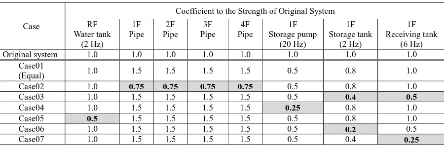
The values indicated in the Table 2 show coefficients to the median strength of the original system. Each case of system has relatively weak equipment components in the system, therefore, the functional loss would be occurred with various patterns depending on system cases. The coefficients of Case01 were adjusted so that each equipment component has the same contribution to the damage of entire system. The systems of Case02~Case07 have relatively weak components compared with that of Case01. The weak equipment components of each system case are shaded in Table 2.
In the evaluation of building functional loss, the damage probability of each component was calculated by comparing their structural responses of their location with their strength. Concretely, the damage probabilities of tanks and pump were evaluated based on the acceleration floor response (1% damping) corresponding to their natural frequency, which are listed as “Damage index” in Table 1. Those of pipes were evaluated based on the story drift angle of their location.
Table 1: The strength and the damage index for each equipment of an original system
Equipment Location Damage index Strength
Median Log-standard deviation (loge)
Water tank RF Acc. Response 2Hz 3500 (cm/s2) 0.15
Pipes 1~4F Drift Angle 1/150 (rad.) 0.20
Storage pump 1F Acc. Response 20Hz 1400 (cm/s2) 0.15
Storage tank 1F Acc. Response 2 Hz 1400 (cm/s2) 0.15
Receiving tank 1F Acc. Response 6 Hz 2200 (cm/s2) 0.15
Table 2 : System cases and their coefficient for each equipment.
Case
Coefficient to the Strength of Original System RF
Water tank (2 Hz)
1F Pipe
2F Pipe
3F Pipe
4F Pipe
1F Storage pump
(20 Hz)
1F Storage tank
(2 Hz)
1F Receiving tank
(6 Hz)
Original system 1.0 1.0 1.0 1.0 1.0 1.0 1.0 1.0
Case01
(Equal) 1.0 1.5 1.5 1.5 1.5 0.5 0.8 1.0
Case02 1.0 0.75 0.75 0.75 0.75 0.5 0.8 1.0
Case03 1.0 1.5 1.5 1.5 1.5 0.5 0.4 0.5
Case04 1.0 1.5 1.5 1.5 1.5 0.25 0.8 1.0
Case05 0.5 1.5 1.5 1.5 1.5 0.5 0.8 1.0
Case06 1.0 1.5 1.5 1.5 1.5 0.5 0.2 0.5
Case07 1.0 1.5 1.5 1.5 1.5 0.5 0.4 0.25
The 4th story of reinforced concrete structure was assumed as a target building, which is the same with Igarashi et al (2015). The structure was modelled as multi-mass shear system, where the elastic natural frequency was 4.3Hz. The basement of the structure was fixed on the engineering bedrock. For the non-liner characteristics of shear spring, tri-liner characteristics was applied.
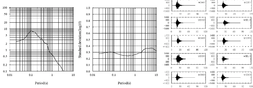
The input ground motions of 2736 waves were generated from a seismic source “Minami-Kanto” region, which is one of the seismic sources contribute to hazard at the target site, Oarai in Japan. The magnitude is 7.1, the distance is 45~65km. The uncertainties of seismic-source characteristics are considered based on the logic tree and Monte Carlo simulation. The maximum acceleration of 2736
waves distributes from 20 to 1600 cm/s2. Figure 4 shows the median response spectra (5% damping),
liner analyses (SHAKE). As for the details, see the preceding study by Nishida et al. (2013, 2016), Takada et al. and Igarashi et al.(2015).
Table 3 shows the candidate seismic intensity indices in this study. These indices are generally used for representing the fragility curve of structure or equipment (Oi et al., 2003), and they can be evaluated from each ground-motion time history. The proposed method is applied for each system case to confirm whether the optimal seismic intensity indices can be properly detected based on the proposed method.
Figure 4. Stochastic values of acceleration response of 2736 waves and examples of time history.
Table 3: Candidate seismic intensity index.
Candidate seismic intensity indices Equations Reference
ACC Maximum acceleration ACCmaxa(t) -
CAV Cumulative absolute velocity
n
i t t
i
i
dt t a CAV
1
1
)
( EPRI(1991),Ochiai(2014)
VEL Maximum velocity VELmaxv(t) -
E Incident energy density
0 2
) (tdt v V
E s Hirai and Sawada(2012)
S.I. Spectrum intensity
2.51 .
0 ,0.05( )
.
.I S T dT
S V Housner(1965)
M.S.I. Modified spectrum intensity
0.51 .
0 ,0.05( )
. .
.SI S T dT
M A Kobayashi et al.(1978)
Ajma JMA effective acceleration 10Ijma0.94/2
jma
A Tong and Yamazaki(1996)
RSP f f Hz response acceleration 1% Damping -
The Results of Validation
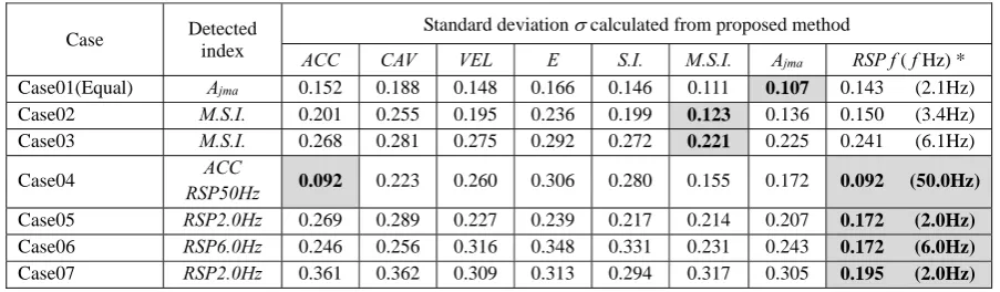
Table 4 shows the standard deviation of the discrepancies for each candidate seismic intensity
index. In each case, the index shaded its indicates the optimal seismic indices detected according to the
proposed method.
The index detected with Case01 is Ajma, JMA effective acceleration. There was no specific
equipment components which especially contribute to the damage of system of Case01, therefore, it is
selected. The index detected with Case02 where the pipes on the 1~4th floor are contribute to the damage
of system is M.S.I., the modified spectrum intensity. This is because the story drift angles involve the
effects of non-linear characteristics of the structure, it is considered that the index M.S.I. which contains
the response components of lower 4.3Hz (upper 0.233s) has good correlation with the damage of pipes.
Similarly, the index detected with Case03 is M.S.I. which involves the response of 2.0Hz and 6.0Hz. As
for Case04, The indices ACC and RSP50Hz were detected. It was expected that the index RSP20Hz might
be selected because the damage of pump which is the weakest component in the system can be indicated by the acceleration response of 20Hz. It is considered that the soil characteristics from free rock to basement of structure affected the periodical differences of detected index. As for Case05~Case07, the indices which represent the damage of entire system were properly detected. For example, Case05 and Case06 where the one of the components in parallel system on 1st floor is weak, the index which indicates the damage of the other component in parallel system was detected. Case07 where the one of the component in series system is weak, the index which indicates the damage of the weak component was detected. According to these results, it was confirmed that the optimal seismic intensity index can be properly detected based on the proposed method.
Table 4 : The optimal indices detected by the proposed method.
Case Detected
index
Standard deviation calculated from proposed method
ACC CAV VEL E S.I. M.S.I. Ajma RSP f ( f Hz) *
Case01(Equal) Ajma 0.152 0.188 0.148 0.166 0.146 0.111 0.107 0.143 (2.1Hz)
Case02 M.S.I. 0.201 0.255 0.195 0.236 0.199 0.123 0.136 0.150 (3.4Hz)
Case03 M.S.I. 0.268 0.281 0.275 0.292 0.272 0.221 0.225 0.241 (6.1Hz)
Case04 RSP50Hz ACC 0.092 0.223 0.260 0.306 0.280 0.155 0.172 0.092 (50.0Hz)
Case05 RSP2.0Hz 0.269 0.289 0.227 0.239 0.217 0.214 0.207 0.172 (2.0Hz)
Case06 RSP6.0Hz 0.246 0.256 0.316 0.348 0.331 0.231 0.243 0.172 (6.0Hz)
Case07 RSP2.0Hz 0.361 0.362 0.309 0.313 0.294 0.317 0.305 0.195 (2.0Hz)
* Standard deviation of response spectrum at the frequency f where the spectra show the minimum for the frequency 0.1~50Hz.
NUMBER OF GROUND MOTIONS FOR SELECTING OPTIMAL SEISMIC INDEX
In previous chapter, the optimal seismic intensity indices were detected based on the results of damage probabilities of 2736 waves. However, it is desired that optimal seismic intensity index can be detected based on smaller sampling numbers of waves as possible. In this chapter, it was investigate how many waves are needed for detecting the optimal seismic intensity index.
Firstly, the results of the damage probabilities of system due to N waves (N=3~300) were
randomly selected from the results due to 2736 waves of ground motions, and then the optimal seismic
intensity index is detected based on the results of N waves. If the detected index with N waves was the
same with that with 2736 waves, it can be said that the sampling number N is enough to evaluate an
optimal seismic intensity index based on the proposed method.
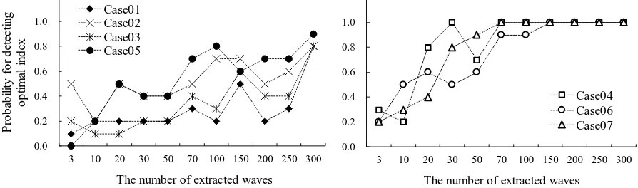
Here, the hitting probabilities of detecting optimal index which is the same with 2736 waves were
examined by 10 times of trial of selecting an optimal indices using N waves.
The results of each case were shown in Figure 5. The results of Case04, 06, 07 indicate that several tens of waves are needed to obtain about 80~90 % of hitting probability. On the other hand, the results of Case01, 02, 03, 05 indicate that several hundred waves are needed to obtain appropriate indices.
Table 5 shows the results of “index A” which shows the smallest of all candidate indices and
the “index B” which shows the 2nd smallest in each case. Their differences of and the number of
of waves tend to be selected the similar indices with index A and index B (e.g. M.S.I. and Ajma), therefore
their differences of are relatively small. This is because large numbers of ground motions are needed to
classify the standard deviation of these similar indices. In any system cases, it was indicates that if there
were several tens or hundreds of ground motions, relatively reasonable seismic intensity index can be detected based on the proposed method. However, in order to select an optimal index from smaller number of waves, the candidate indices is recommended to be prepared some indices with dissimilar characteristics instead of indices with similar characteristics.
0.0 0.2 0.4 0.6 0.8 1.0
3 10 20 30 50 70 100 150 200 250 300
P
roba
bi
lit
y
f
o
r
de
te
ct
in
g
opt
im
al
i
n
de
x
The number of extracted waves Case01
Case02 Case03 Case05
0.0 0.2 0.4 0.6 0.8 1.0
3 10 20 30 50 70 100 150 200 250 300
The number of extracted waves Case04 Case06 Case07
Figure 5. Hitting probabilities of detecting expected optimal index.
Table 5. Required number of waves derived from the differences of for two optimal indices.
Case Index A ( the smallest ) Index B ( the 2nd smallest ) |A-B|
The number of waves when prob. exceeds 80 %
Case01 Ajma = 0.107 M.S.I. = 0.111 0.004 100 waves
Case02 M.S.I. = 0.123 Ajma = 0.136 0.013 upper 300 waves
Case03 M.S.I. = 0.221 Ajma = 0.225 0.004 upper 300 waves
Case04 ACC RSP50Hz = 0.092 M.S.I. = 0.155 0.063 20 waves
Case05 RSP2.0Hz = 0.172 Ajma = 0.207 0.035 upper 300 waves
Case06 RSP6.0Hz = 0.172 M.S.I. = 0.231 0.059 70 waves
Case07 RSP2.0Hz = 0.195 Ajma = 0.305 0.099 30 waves
EFFICIENT WORKFLOW OF RISK ASSESSMENT BASED ON GROUND MOTIONS WITH FAULT MODELS
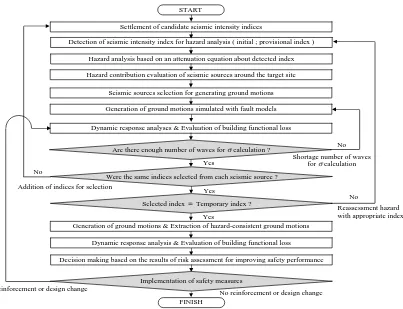
Figure 6 shows the workflow of seismic risk assessment of structure utilizing ground motions based on fault models. In the first half of the Figure 6, the selecting flow of optimal seismic intensity index based on the proposed method is shown. The general seismic intensity index such as a maximum acceleration or a maximum velocity can be adopted as an initial index for seismic hazard analysis. Starting the ground-motion generation for the seismic sources which contribute to the seismic hazard based on the provisional index, the time-history response analyses input these motions are also conducted. Then, the damage probabilities of the equipment system is evaluated comparing the strength of each component of the system with the maximum responses of them. After generating about several tens or
hundreds waves, the seismic intensity index which has the smallest is detected as an optimal indices
based on proposed method.
indicated building functional loss, the ground motions are generated from the hazard-contributed seismic sources, and then the building functional loss was evaluated with these ground motions.
In the second half of the Figure 6, the decision making flow of safety measures such as a reinforcement or a design change of building is shown. If some safety measures would be conducted based on the result of the building functional loss, the effects of the safety measures can be validated by comparing renewed models of structure and equipment system with the previous models.
Figure 6. Workflow of efficient seismic PRA utilizing ground motions with fault models.
CONCLUSION
In this paper, an efficient evaluation method for seismic PRA utilizing ground-motion time histories simulated with fault models was proposed. The proposed method can detect an optimal seismic intensity index which has the best correlation with a seismic risk of a facility. This enables us to reduce the sampling number of ground motions because the ground-motion generations can be conducted focusing on the risk-contributed seismic sources. In this study, a building functional loss due to seismic
damages of equipment system was defined as a seismic risk. The standard deviations , that are the
discrepancies between the damage probabilities of the system according to the order of themselves and those according to the order of candidate seismic intensity indices, were evaluated, and then the seismic
intensity index which shows the smallest was detected as an optimal index.
In order to validate the applicability of the proposed method, some cases of equipment system were examined. Each case of the system has relatively weak equipment component which contributes to the damage of the entire system. The proposed method was adopted to these system cases, and it was confirmed that the proposed method can properly select the optimal index. It was also estimated how
Hazard analysis based on an attenuation equation about detected index
Generation of ground motions simulated with fault models Hazard contribution evaluation of seismic sources around the target site
START
No reinforcement or design change FINISH
Implementation of safety measures Addition of indices for selection
Reassessment hazard with appropriate index Shortage number of waves
for calculation
Dynamic response analysis & Evaluation of building functional loss Selected index = Temporary index ?
Were the same indices selected from each seismic source ? Settlement of candidate seismic intensity indices
Detection of seismic intensity index for hazard analysis ( initial ; provisional index )
Seismic sources selection for generating ground motions
Dynamic response analyses & Evaluation of building functional loss
Are there enough number of waves for calculation ?
Generation of ground motions & Extraction of hazard-consistent ground motions
Decision making based on the results of risk assessment for improving safety performance
Reinforcement or design change
Yes
No
Yes No
Yes
many ground motions are required to detect an optimal seismic intensity index. It was clarified that about several tens or hundreds of ground motions are required, and that the number of ground motions depends on the differences of characteristics of the candidate indices.
Finally, an efficient workflow of seismic risk assessment for a general facility utilizing ground motions simulated with fault models was presented.
ACKNOWLAGEMENT
The data of ground motions in this paper were provided from Japan Atomic Energy Agency. The author shows gratitude for kindly supports.
REFERENCES
Atomic Energy Society of Japan, (2007), “A standard for Procedure of Seismic probabilistic Safety Assessment (PSA) for nuclear power plants”
Electric Power Research Institute., (1991). “Standardization of the Cumulative Absolute Velocity”, EPRI TR-100082
Hirai and Sawada, (2012). “Validation of Predicted Strong Ground Motion Based on Energy Index of Seismic Wave”, Journal of JAEE, 31-42
Housner, G., W.,(1965). “Intensity of Earthquake Ground Shaking Near the Causative Fault”, Proc. of 3rd WCEE, 94-115
Igarashi, S., Sakamoto, S., Nishida, A., Muramatsu, K., and Takada, T. (2015), “Structural Response by Ground Motions From Sources with Stochastic Characteristics,” Proc. of ICONE-23
Igarashi, S., Sakamoto, S., Nishida, A., Muramatsu, K., and Takada, T. (2015), “Effects of Source Characteristics Uncertainties on Seismic Intensity and Structural Response (in Japanese),” Journal of AIJ, Vol.81, No.721, 425-435
Igarashi, S., Sakamoto, S., Uchiyama, Y., Yamamoto, Y., Nishida, A., Muramatsu, K. and Takada, T. (2015) “Seismic Damage Probability by Ground Motions Consistent with Seismic Hazard ”, Proc. of SMiRT-23
Kobayashi et al.,(1978). “ Study on Spectrum Intensity on Seismic Bedrock Around Seismic Sources (in Japanese)”, AIJ, 553-554
Nishida, A., Igarashi, S., Sakamoto, S., Uchiyama, Y., Yamamoto, Y., Muramatsu, K., and Takada, T. (2013). “Characteristics of Simulated Ground Motions Consistent with Seismic Hazard, ” Proc. of SMiRT-22
Nishida, A., Igarashi, S., Sakamoto, S., Uchiyama, Y., Yamamoto, Y., Muramatsu, K., and Takada, T. (2015). “Characteristics of Simulated Ground Motions Consistent with Seismic Hazard,”, Elsevier, UK
Ochiai, K., (2014). “Capacity of NPPs against Earthquake & Proposals to Prepare for Post-Earthquake Electric Supply(in Japanese)”, Journal of the Atomic Energy Society Japan, Vol.56, No.2, 70-74 Oi, M., (2003). “Study on Probabilistic Estimation Method of Seismic Damage for Structures (in
Japanese)”, Technical Note of the National Research Institute fir Earth Science and Disaster Prevention, No.237
Sugawara et al. ,(1999). “The study of the relation between measured seismic intensity and the other indexes(in Japanese)”, AIJ, 175-176
Takada, T., et al. (2014). “Comparison with Ground Motions Generated by Different Methods Considering Source Uncertainties (in Japanese)”, AIJ, 1-2.
The Building Center of Japan, (2014), “A Guideline of Seismic Design and Construction for Building Facility (in Japanese)”