Temperature Distribution Measurement by Michelson Interferometer

Temperature Distribution Measurement by

Michelson Interferometer

Anooplal B

, Binoy Baby

Dept. of Mechanical Engineering, SJCET, Pala, Kerala, India1,2

ABSTRACT: Interferometry is a non-intrusive technique becoming increasingly popular in engineeringmeasurement.

Michelson interferometry is one among those aligned to detect the measurement of air temperature around a flame by non-intrusive technique. The temperature of air at a reference point is recorded by a single thermocouple placed at a distance from the heat source. Interference pattern obtained are analyzed by using a camera and image processing in MATLAB software. From the observation results, it clearly shown that the change of air temperature in one arm of the interferometer will result in the fringe deformation of the interference pattern. Comparison of initial and deformed fringe patterns using image processing technique, the temperature around the heat source can be measured in the medium surrounded by the flame. Using this technique temperature distribution of a region and temperature at any point in the region can be determined from the temperature profiles. This is achieved even without disturbing the flow of the medium and performance of the device being studied. Thus equipment can be tested efficiently and measure the proper dissipation of heat in the devices.

KEYWORDS: interferometry, image processing, heat dissipation

I. INTRODUCTION

Interferometry is a family of techniques in which waves, usually electromagnetic are superimposed in order to extract information about the waves. The principle of superposition to combine waves in a way that will cause the result of their combination to have some meaningful property that is diagnostic of the original state of the waves. When two or more propagating waves of same type are incident on the same point, the total displacement at that point is equal to the point wise sum of the displacements of the individual waves. The resultant waves are constructive interference or destructive interference depends on the point of contact.

Recent advances in microelectronic field have made it necessary to develop effective new methods capable of thermal management of compact heat producing devices. Due to their compact and restricted surface area, it produces high heat flux. Shoban C.B and Peterson, G.P,[1] explained micro scale and nano scale heat transfer in engineering measurements. For a wide class of applications, where temperature differences are not abnormally large, interferometry appears to be a versatile tool for accurate measurement of three-dimensional unsteady temperature fields, and with some modification for velocity fields by Mehandale et.al [2]. Rammohan et.al [3] describes the natural heat transfer by Mach-Zehnder Interferometer and Differential interferometer. Differential Interferometer shows fairly good heat transfer and temperature than the other. According to Binoy et.al [4], forced convection in compact mini-channel with apparent rectangular shape is analysed with finite element method and calculation is validate using Michelson Interferometry. Binoy and Soban [5] did forced convection in a meso-channel with irregular cross section by finite difference solution. The numerical results are compared with the analytical results obtained by Mach-Zehder Interferometry. Minnett et.al [6] measures the radiometric marine air temperature by Marine-Atmospheric Emitted Radiance Interferometer. This approach deployed in wide range of conditions and helped to determine some of the errors characteristics of the standard measurement.

II. EXPERIMENTALSTUDY

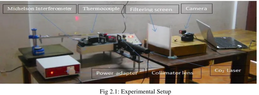
As the experimental set up shown in the fig. 2.1, Osaw carbon dioxide laser unit and an adapter were connected to the electric power socket. After switching on, the carbon dioxide laser beams were passed through a collimator lens which further increase the intensity of the beam and make it more precise. A beam splitter splits the beam into two parts namely transmitted beam and reflected beam. These beams hit the mirrors at the two extremes thro ugh lenses provided in between them. The returning beams are recombined and a converging lens is provided. A light filtering arrangement is provided for adjusting the brightness to make it easier for image to be captured on a camera at a better quality. A laptop was provided to operate the camera remotely since manual operation of the camera can lead to small miss-alignment of same pixels in consequent pictures taken. The fringes are obtained by adjusting the course screws. It takes a very high time for adjusting both these screws as even a minute disturbance could lead to the distortion of the fringe pattern. The fans were switched off in the room which was closed to prevent the disturbances that affect the medium in order to obtain a clear fringe. The screws are then adjusted to obtain different types of fringes namely horizontal, inclined and vertical.

Fig 2.1: Experimental Setup

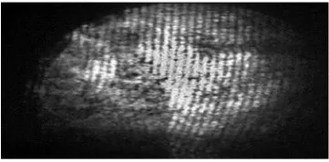
The heat source used in this experiment is a lighted candle. The images were captured by using a camera with and without lighting the heat source. The laser light source is made to pass through a collimator lens to increase its intensity and it hits a beam splitter which splits the beam into two half, a reflected beam and a transmitted beam, which hit the mirrors and recombines at the beam splitter to give an interference fringe pattern on the screen. During the experiment, it was found that the interference pattern obtained on the screen was much brighter than expected. So the camera could not capture the image in detail. This led to create a filter paper onto which the interference pattern was directed to fall dark and bright bands that could be obtained clearly through it by properly adjusting the filter paper and thus reducing the intensity. For processing the images using the MATLAB software, the images must be identical in the sense that pixels for which the position of the image processer should not be changed and for that we have connected the camera with a laptop in order to capture the image remotely without shaking. The images were captured with and without the heat source for horizontal, inclined and vertical fringe settings. The obtained images are respectively shown below.

Fig.2.4: Inclined fringe without heat source Fig.2.5: Candle flame in the inclined fringe setting

Fig. 2.6: Vertical fringe without heat source Fig. 2.7: Candle flame in the vertical fringe setting

III.ANALYSIS

From the experimentation, a pair of images from each type of fringe was obtained. Within the software, the data contained in the images were converted to matrix format. These images contained constant temperature lines between the heat source and thermocouple called isotherms. The intensity profile of the resultant image was drawn over the distance between the centre of the candle and the thermocouple. Image containing the heat source (lighted candle) and a slip gauge used to know its length was taken and this image was processed by the software to determine the width of the flame. The pixel coordinates at the two extremes of the gauge and the pixel coordinates of the lighted candle flame were taken. Since the dimension of the gauge is known from the pixel coordinates, the known dimension of the slip gauge determined the length of one pixel. With this pixel length, it is easy to determine the width of the flame. This width is to be used in equation to determine the temperature distribution. To find temperatures at each isotherm by using MS Excel software, a graph plotted and polynomial was fitted. The obtained polynomial is shown below



 



With reference the Lawrence-Lawrence relation is used to find the temperature at isotherms.

r

polynomial (T ) 1

polynomial (T) [1 (a s)] (2)

T r : Reference temperature, T : Temperature to be measured, s : Isotherm number

2

r

n 1 1

a

C L polynomial(T )

n 1

 

  



 (3)

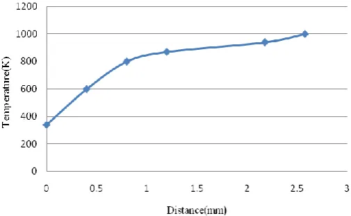
The pixel coordinates of each fringe were determined. By considering the pixel at thermocouple to be reference zero, the relative pixel distances to the isotherms were determined. As the length of the pixel found earlier, it can be used for finding out the distance of different isotherm (in mm) from the thermocouple located as the point at which reference temperature is taken. Using the length and temperature observed above, the graph is plotted.

.

IV.RESULTS

IV.I Horizontal

The images obtained from the experiment conducted using horizontal fringes were compared in MATLAB to obtain fig 4.1. It contains dark and light bands above the horizontal fringes. The narrow dark bands among them are called isotherms since they are constant temperature regions. The intensity profile drawn between the centre of heat source and thermocouple is shown in fig 4.2. By analyzing this intensity plot neglecting its sharp fluctuations, it can be seen the crust indicating high brightness of light bands and the troughs represent the isotherms. Fig 4.3 is a plot between temperatures of isotherm and their distance from the reference point. Lowest temperature is the reference temperature and highest is that of the isotherm nearest to the heat source.

Fig 4.1: Isotherms formed on horizontal fringes

Fig 4.2: Intensity profile for horizontal fringes Fig 4.3: Temperature profile for horizontal fringes

Distance (Pixel)

In

ten

sit

y

(c

d

IV.II Inclined

As same as in the case of horizontal fringes, the fig 4.4 is obtained by minus operation of the pair of images (taken in presence and absence of heat source) from the experiment. But the numbers of fringes obtained are different from those of horizontal. Fig 4.5 is smoother compared to the intensity profile from horizontal fringe.

The crust and trough are easily distinguishable. The distance considered for intensity plot was between the point at which reference temperature is taken and the center of heat source. The reference temperature was higher, but the source temperature obtained was close to that in other type of fringe since the reference length varied. These data were used to plot fig 4.6

Fig 4.5: Intensity profile for inclined fringe

IV.III Vertical

Figure 4.7 is the resultant image that shows isotherms in vertical fringe setting. Figure 4.8 contains equal number of troughs as that of isotherms in. Intensity profile with greater accuracy is obtained when using an image in grey scale rather than using an image in colour. From Lorenz-Lorentz relation, temperatures and data cursor position of isotherms were determined. This data was used to draw fig 4.9. This figure shows a continuous variation (increase) in temperature from reference point to heat source. From this plot, it can be conveniently found the temperature at any point within the given distance limit.

Distance (pixels)

In

ten

sit

y

(Cd

Fig 4.7: Isotherms formed on vertical fringe

V.CONCLUSION

A simple Michelson interferometry was aligned to detect the measurement of air temperature. Using a single thermocouple, temperature of a point far from the heat source is only needed here. Thus, non-intrusive measurement is made possible without disturbing the medium. The interference pattern containing the data regarding the heat distribution was captured as an image. This was analyzed on MATLAB to obtain an intensity plot and a resultant image. The resultant image shows the positions of isotherms. Lawrence-Lawrence relation was used to determine the temperatures at these isotherms. Positions of the isotherms were determined using data cursor on MATLAB. From the temperature and position, temperature plots were drawn. The temperature of any point between reference and heat source can be determined using the temperature plot. Thus temperature distribution is measured without affecting the medium. Images are obtained from experiment conducted by vertical, horizontal and inclined fringes. Measured temperature is almost same for these different fringes alignments. Therefore, any of these fringe settings can be used. This technique can be used to measure the heat dissipation capacity of any equipment without the measuring equipment itself interfering with the performance of the equipment being studied.

REFERENCES

[1]Sobhan, C. B., and Peterson, G. P., Microscale and Nanoscale Heat Transfer-Fundamentals and EngineeringApplications, Taylor and Francis, New York, 2008, pp.

125–190.

[2]Mehendale, S. S., Jacobi, A. M., and Shah, R. K., “Fluid Flow and Heat Transfer at Micro- andMeso-Scales with Application in Heat Exchanger Design,”Applied

Mechanics Reviews, Vol. 53, No. 7, 2000, pp. 105–116. doi: 10.1115/1.3097347 .

[3] Rao,V. R., Sobhan, C. B., and Venkateshan, S. P., “DifferentialInterferometry in HeatTransfer,”Sadhana, Vol. 15, No. 2, 1990, pp. 105–128.

doi:10.1007/BF02760470.

[4] Binoy Baby, Choondal. L, B. Soban, Investigation on Forced convection in Compact Passage with Surface Iregularities,Taylor and Francis ,Heat Transfer

Engineering, 2012,pp.1105-1119.

[5] Binoy Baby, C.B Sobhan, Numerical and Experimental investigation on forced convection in meso-channel with irregular geometryof cross-section, International

journal of Heat and Mass Transfer vol. 70 , 2014, pp. 276-288.

[6] J. Minnett, K. A. Maillet, J. A. Hanafin, and B. J. Osborne, Infrared Interferometric Measurements of the Near-Surface Air Temperature over the Oceans. J. Atmos.