A new approach in building parallel finite field multipliers

University of Windsor University of Windsor

Scholarship at UWindsor

Scholarship at UWindsor

Electronic Theses and Dissertations Theses, Dissertations, and Major Papers

2009

A new approach in building parallel finite field multipliers

A new approach in building parallel finite field multipliers

Mohammadali Sharifan

University of Windsor

Follow this and additional works at: https://scholar.uwindsor.ca/etd

Recommended Citation Recommended Citation

Sharifan, Mohammadali, "A new approach in building parallel finite field multipliers" (2009). Electronic Theses and Dissertations. 8128.

https://scholar.uwindsor.ca/etd/8128

NOTE TO USERS

This reproduction is the best copy available.

A NEW APPROACH IN BUILDING PARALLEL FINITE

FIELD MULTIPLIERS

by

Mohammadali Sharifan

A Thesis

Submitted to the Faculty of Graduate Studies

through the Department of Electrical and Computer Engineering

in Partial Fulfillment of the Requirements for

the Degree of Master of Applied Science at the

University of Windsor

Windsor, Ontario, Canada

2009

1*1

Published Heritage Branch

395 Wellington Street OttawaONK1A0N4 Canada

Bibliotheque et Archives Canada Direction du

Patrimoine de I'edition

395, rue Wellington OttawaONK1A0N4 Canada

Your file Votre r$f6rence ISBN: 978-0-494-57623-6 Our file Notre reference ISBN: 978-0-494-57623-6

NOTICE:

AVIS:

The author has granted a

non-exclusive license allowing Library and Archives Canada to reproduce, publish, archive, preserve, conserve, communicate to the public by

telecommunication or on the Internet, loan, distribute and sell theses

worldwide, for commercial or non-commercial purposes, in microform, paper, electronic and/or any other formats.

L'auteur a accorde une licence non exclusive permettant a la Bibliotheque et Archives Canada de reproduire, publier, archiver, sauvegarder, conserver, transmettre au public par telecommunication ou par ['Internet, preter, distribuer et vendre des theses partout dans le monde, a des fins commerciales ou autres, sur support microforme, papier, electronique et/ou autres formats.

The author retains copyright ownership and moral rights in this thesis. Neither the thesis nor substantial extracts from it may be printed or otherwise reproduced without the author's permission.

L'auteur conserve la propriete du droit d'auteur et des droits moraux qui protege cette these. Ni la these ni des extra its substantiels de celle-ci ne doivent etre imprimes ou autrement

reproduits sans son autorisation.

In compliance with the Canadian Privacy Act some supporting forms may have been removed from this thesis.

Conformement a la loi canadienne sur la protection de la vie privee, quelques

formulaires secondaires ont ete enleves de cette these.

While these forms may be included in the document page count, their removal does not represent any loss of content from the thesis.

Bien que ces formulaires aient inclus dans la pagination, il n'y aura aucun contenu manquant.

1+1

Author's Declaration of Originality

I hereby certify that I am the sole author of this thesis and that no part of this thesis has

been published or submitted for publication.

I certify that, to the best of my knowledge, my thesis does not infringe upon anyone's

copyright nor violate any proprietary rights and that any ideas, techniques, quotations, or

any other material from the work of other people included in my thesis, published or

otherwise, are fully acknowledged in accordance with the standard referencing practices.

Furthermore, to the extent that I have included copyrighted material that surpasses the

bounds of fair dealing within the meaning of the Canada Copyright Act, I certify that I

have obtained a written permission from the copyright owner(s) to include such

material(s) in my thesis and have included copies of such copyright clearances to my

appendix.

I declare that this is a true copy of my thesis, including any final revisions, as approved

by my thesis committee and the Graduate Studies office, and that this thesis has not been

Abstract

A new method for building bit-parallel polynomial basis finite field multipliers is

proposed in this thesis. Among the different approaches to build such multipliers,

Mastrovito multipliers based on a trinomial, an all-one-polynomial, or an

equally-spaced-polynomial have the lowest complexities. The next best in this category is a conventional

multiplier based on a pentanomial. Any newly presented method should have complexity

results which are at least better than those of a pentanomial based multiplier. By applying

our method to certain classes of finite fields we have gained a space complexity as

n2 + H - 4 and a time complexity as TA + ([ log2(n-l) ]+3)rx which are better than the

lowest space and time complexities of a pentanomial based multiplier found in literature.

Therefore this multiplier can serve as an alternative in those finite fields in which no

Acknowledgments

T would like to thank Dr. Huapeng Wu for all the help and support that he gave me as my

supervisor, and for always encouraging me through the hard times that I had during this

research project.

I also want to thank Dr. Henry Hu for precisely reviewing my work and Dr. Sazzadur

Chowdhury for his valuable advice and comments.

I cannot be grateful enough to my parents for all the sacrifices they made to give me

whatever I need to gain my goals.

Table of Contents

Abstract iv

Dedication.. v

Acknowledgments vi

List of Tables ix

List of Figures x

1 Introduction 1

1.1 Motivation 1

1.2 Thesis Outline 3

2 Mathematical Background 5

2.1 Fundamental Concepts 5

2.2 Modular Arithmetic 8

2.3 Finite Fields 11

2.4 Polynomials and Finite Fields 12

2.5 Extension Finite Fields 16

2.6 Basis in Finite Fields 19

2.7 Finite Field Multiplication in Polynomial Basis 20

2.8 Multiplier Architecture and Complexity 24

3 An Overview of Finite Field Multipliers 26

3.1 Parallel Finite Field Multipliers 27

3.2 Serial Finite Field Multipliers 50

4 New Finite Field Multiplier 57

4.1 Introduction 57

4.2 Multiplier Architecture 59

4.3 Applying the New Method to Classes of Finite Fields 68

4.3.1 Review of Three Classes of Finite Fields 69

4.3.2 Results Related to Type I Polynomials 75

4.3.3 Results Related to Type II Polynomials 78

4.3.4 Results Related to Type III Polynomials 80

4.4 Comparisons 81

5 Conclusion 82

5.1 Summary of contributions 82

5.2 Future Work 83

References 84

List of Tables

Table 2.1 Addition in GF(23) 18

Table 2.2 Multiplication in GF(23) 18

Table 2.3 Multiplicative Inverse Elements in GF(2 ) 19

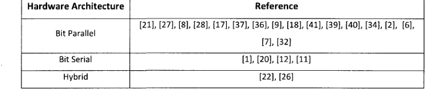
Table 3.1 Finite Field Multipliers Based on Hardware Architecture 54

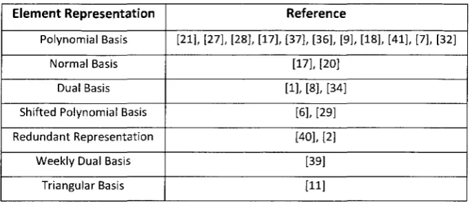
Table 3.2 Finite Field Multipliers Based on Element Representation 55

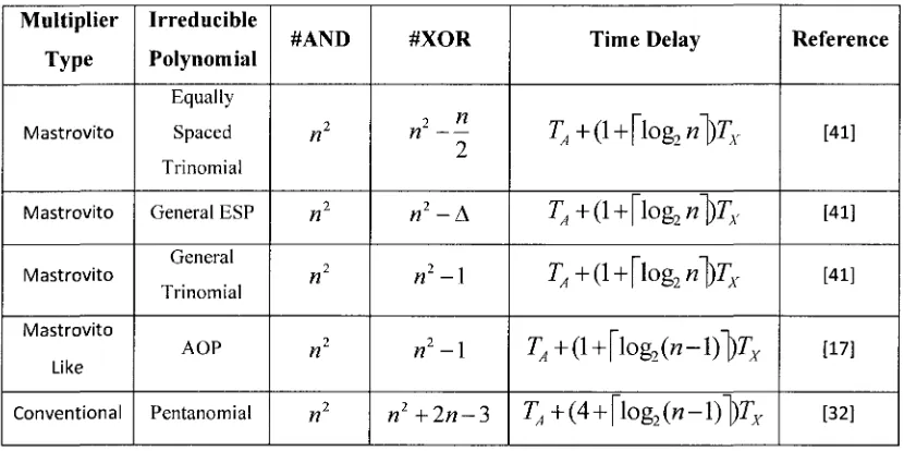
Table 3.3 Best Complexities of Different Finite Field Multipliers 56

Table 4.1 Complexity Results of a Type I Multiplier 78

Table 4.2 Complexity Results of a Type II Multiplier 79

Table 4.3 Complexity Results of a Type III Multiplier 81

List of Figures

Figure 2.1 Arithmetic Operations in Z6 10

Figure 2.2 Arithmetic Operations in GF(5) 12

Figure 3.1 Reduction Array for a General Trinomial 36

Figure 3.2 Reduction Array for x" + xm+1 + xm +x + 1 43

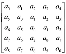
Figure 3.3 A 5 * 5 Toeplitz Matrix 49

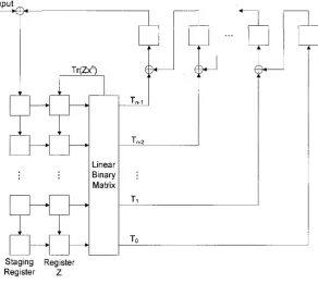
Figure 3.4 Berlekamp Multiplier 51

Figure 3.5 Massey-Omura Serial Multiplier 54

Figure 4.1 V Matrices of GF(25) with f(x) = x5 + x2 +1 65

Figure 4.2 Proposed Multiplier Architecture 67

Figure 4.3 Transfer Matrix of a Type I Polynomial 71

Figure 4.4 T Matrix of a Type II Polynomial 72

Figure 4.5 T Matrix of a Type III Polynomial 75

1 Introduction

1.1 Motivation

In the current age of information technology, while the internet is growing very fast in

almost every aspect of life; electronic communication of very private and important data

is a common task. Consequently, network security has become a primary demand for IT

service providers and users. No matter what the application is, from sharing family

pictures in a social network to sending important customer lists through a business email

or checking your bank account balance online, information transaction should be done

with a very high level of confidentiality. Secure transactions are even more vital when it

comes to e-commerce, online money transactions or governmental information

transactions such as social insurance numbers or tax returns. Almost all required network

security services can be achieved by Cryptography [35].

Encryption is one common cryptography algorithm which means scrambling the data in a

way that only authorized users with proper authorization (a necessary key) can

unscramble it. Cryptography algorithms fall into two main categories: symmetric key and

public key.

Symmetric key cryptosystems rely on a key distribution center which provides a special

required keys for a network grows very fast by increasing the number of users. Therefore,

in large systems symmetric key cryptosystems encounter key management and key

distribution problems. This problem led to the introduction of the public key cryptography

by Diffie and Hellman in 1976 [3].

In a public key network, each user is assigned two special keys. One key is kept private

while the other is known to all the other users in the network. Any message addressed to

the user is scrambled with the user's public key. However, in order to unscramble this

data, only the user's private key is applicable. Different methods have been introduced

for public key. In 1978 Rivest, Shamir and Adleman [33] introduced the so-called RSA

algorithm which is by far the most popular public key algorithm. About a decade later in

1985 El-Gamal [4] introduced another technique in cryptography named after himself. At

the same time Koblitz [16] and Miller [24] independently introduced the elliptic curve

cryptography (ECC) where finite fields came into play. This method is based on the

group of points on an elliptic curve (EC) over a finite field.

Despite the fact that the vast majority of the products and standards that use public key

cryptography for encryption use the RSA method, ECC is more efficient compared to

RSA. This is because ECC can offer equal security with a far smaller key size, hence

reducing processing overhead. Since the RSA standard key length has recently greatly

increased, the issue of the key length has come more into attention, especially that the

increase in key length has put a burden on e-commerce sites that conduct large number of

secure transactions. This is leading to a vast replacement of RSA by ECC in many

different security products in hardware and software.

Elliptic curve cryptography (ECC) is based on the elliptic curve discrete logarithm

problem [10]. EC calculation over a finite field is based on finite field addition,

subtraction, multiplication, squaring and division amongst which multiplication is the

Although implementing cryptography algorithms in the software level is much easier,

they are considerably slower compared to hardware implementations. This will

effectively slow down its processing and increase the consumption of the valuable time of

the main processor of the hosting system. On the other hand, the hardware

implementation of a cryptosystem will result in faster processors and the opportunity to

have larger key lengths. The advantages of these characteristics can be clearly seen where

there is a large volume of secure transactions. Hence hardware implemented

crypto-processors result in a higher level of security with a better performance.

Efficient hardware implementation of ECC systems highly depends on the efficiency of

finite field multiplication. This is due to the fact that when calculating the speed of an

elliptic curve processor, finite field multiplication is considered to be the most time

consuming operation. Finite field addition (and in some systems squaring) is considered

to be almost free compared to multiplication [5]. The importance of improving finite field

multiplication algorithms provides the main motivation of this research.

In this thesis a new efficient parallel finite field multiplier is proposed which can be used

as an alternative for present methods of multiplication in hardware implementation of

elliptic curve cryptosystems.

Application of finite field multipliers is not restricted to elliptic curve cryptography.

Before the introduction of ECC, finite fields had come into attention in coding theory and

error detecting codes especially in Reed-Solomon encoders [30]. Finite field arithmetic is

also used in combinatorial designs [38], and computer algebra [19]. This shows the

extensive application of finite field multiplication algorithms. Nevertheless this thesis

mainly focuses on the application of finite field in public key cryptography.

1.2 Thesis Outline

Chapter 2 gives an introduction to finite fields and the arithmetic within these fields. It

explains different methods of multiplication. Various classes of finite fields are

introduced and different methods of representing elements in finite fields are reviewed.

Chapter 3 provides a comprehensive survey on the state-of-art technologies on building

finite field multipliers. It explains different types of implementations of finite field

multipliers and compares pros and cons of each method. It also provides different types

of fields used in finite field multipliers and since this thesis proposes a parallel

polynomial basis finite field multiplier all the similar existing multipliers are provided

with their exact space and speed complexities.

Chapter 4 introduces the new method of finite field multiplication. It provides complete

hardware architecture for this multiplier. Also some recently introduced types of finite

fields are reviewed and the new architecture of multiplier is applied to these fields.

Finally it provides the results of this multiplier for those fields in terms of space and time

complexity of the hardware.

In the end, Chapter 5 presents the concluding remarks surrounding our proposed method,

2 Mathematical Background

2.1 Fundamental Concepts

Groups, rings and fields are the fundamental elements of a branch of mathematics called

abstract algebra. In this branch we deal with certain sets and their elements on which we

can operate algebraically; meaning that by combining two elements of the set in several

ways a third element of the set can be obtained. There are certain rules which control

these operations. It is important to note that although the notations of these operations are

usually similar to addition or multiplication; in abstract algebra we are not limited to

ordinary arithmetical operations.

Groups

Definition 2.1 A group G; here denoted by {g, *}, is a set G together with a binary

operation * on G such that the following properties hold:

1. Closure; that is, for all a, b in G, a * b is in G

2. Associativity; that is, for all a, b, c in G, a * (b * c) = (a * b) * c

3. Unity element; there is an element e in G such that for all a in G, a * e = e * a = a

It is important to note that "*" is not necessarily "x" although it could be "x" or "+".

Commutative Group

If the group also satisfies

5. For all a, b in G, a * b = b * a

Then the group is called commutative or abelian.

Finite Group

If the group contains finite number of elements then it is called & finite group. The order

of a group is the number of elements in the group.

Cyclic Group

Exponentiation in the group is defined as repeated application of the group operator. Here

if a fixed element a exists in G in a way that every element in G is a power ak, then the

group is called cyclic and element a is called the generator of the group.

If the operation of the group is "+ " then the group is called additive and the unity

element is represented as "0". If the operation of the group is "x", then the group is called

multiplicative and the unity element is represented by " 1 " .

Rings

Definition 2.2 A ring R; here denoted by {R,+, x}, is a set R and two binary operations

addition and multiplication in a way that the following properties are satisfied:

2. Closure for "x"; that is, for all a, b in R, a x b is also in R

3. Associativity of "x"; that is, for all a, b, c m R, a x (b x c) = (a x b) xc

4. Distributive laws for "x" over "+"; that is, for all a, b, c in R,

ax(b + c) = a x b + a x c and (a + b)xc = axc + bxc

Commutative Ring

If the ring also satisfies

5. For all a, b in R, a x b = b x a

Then the ring is considered commutative.

Integral Domain

If a commutative ring satisfies the following axioms:

6. Unity element for "x"; there is an element " 1 " in R such that for all a in R,

a x 1 = lx a = a

7. No zero divisors; if a, b in R and a x b = 0 then either a = 0 or b = 0

Then it is called an integral domain.

Fields

Definition 2.3 A field F, which we denote by {F,+, x}, is a set of elements with two

binary operations addition and multiplication such that the following properties are hold:

1. F is an integral domain

2. Multiplicative inverse; for all a in F there is an element a'1 in F such that

In other words, a field is a set in which addition, subtraction, multiplication and division

is possible without leaving the set. Division is defined as a / b = a x (b'1) and subtraction

is defined as a- b = a + (-b) in which -b is defined as additive inverse of b.

Finite Field

If the number of elements of the field is finite then it is called a finite field.

2.2 Modular Arithmetic

Dividing any integer a by any positive integer n will result in an integer quotient q and a

remainder r, which is a positive integer. This relationship is demonstrated as:

a = qn + r where 0 < r < n and q = [a/nj (2.1)

In which [x\ is the largest integer less than or equal to x. The remainder r is often referred

to as residue.

"mod" Operator

For an integer a, and a positive integer n; a modn is defined as the residue of a/n.

Congruent Modulo

Two integers a, b are congruent modulo n if a mod n = b mod n and it is written as:

a = b mod n.

Divisor

Residue Class

A Residue class is the set of all integers which are congruent modulo n. Each class is

represented by the smallest non-negative integer in the class. Consider a set Z„ which

contains all non-negative integers less than n. This set contains all the residue classes

modulo n. For example Z3 = {0, 1, 2} shows all residue classes of n = 3. These classes

are:

[0] = {..., -9, -6, -3, 0, 3, 6, 9, ...}

[1] = {...,-8,-5,-2, 1,4,7, 10, ...}

[2] = {...,-7,-4,-1,2, 5, 8, 11,...}

Reducing modulo n

For each integer k, finding the smallest non-negative integer to which k is congruent

modulo n is called reduction modulo n.

By definition, the "mod n" operator maps all integers into Z„. This suggests the idea of

performing arithmetic operations within the confines of this set. This type of arithmetic is

called modular arithmetic and it has the following basic properties:

1. [(a mod n) + (b mod n)] mod n = (a + b) mod n

2. [(a mod n) x (b mod n)] mod n = (a x b) mod n

If we perform this modular arithmetic only on integers in Z„, with the following

properties, it can be seen that Zn is a commutative ring with an identity element for

multiplication:

1. Commutative laws:

i. (a + b) mod n = (b + a) mod n

2. Associative laws:

i. [(a + b) + c] mod n = [a + (b + c)] mod n

ii. [(a x b) x c] mod n = [a x (b x c)] mod n

3. Distributive laws:

i. [a x (b + c)] mod n = [(a x b) + (a * c)] mod n

ii. [a + (b x c)] mod n = [(a + b) x (a + c)] mod n

4. Unity elements:

i. (0 + a) mod n = (a + 0) mod n = a mod n

ii. (1 x a) mod n = (a x ]) mod n = a mod n

5. Additive inverse:

i. For each a in Zn there exists b in Zn such that a + b = 0 mod n

An example would clarify this better. Considering Z<>, the elements of this field are:

{0, 1, 2, 3, 4, 5}. Figure (2.1) shows the arithmetic operations in Z^:

0 0 1 1 2 2 2 3 4 3 3 4 5 0 4 4 5 0 1 2 5 5 0 1 2 3 4 X 0 1 2 3 4 5 0 0 1 0 1 2 0 2 4 3 0 3 0 3 4 0 4 2 0 4 5 0 5 4 3 2 1 a 0 1 2 3 4 5 -a 0 5 4 3 2 1 a-i 1 —_ 5

Figure 2.1 Arithmetic Operations in Zf,

It can be seen that multiplicative inverse doesn't exist for all elements of Z„. The reason

behind that comes from a concept called relatively prime. Two integers are considered to

be relatively prime {co-prime) if their only common positive integer factor is 1. For all a

above example 1 and 5 had a multiplicative inverse in Ze but 2, 3 and 4 didn't because

they have common factors other than 1 with 6 which are 2, 3 and 2 respectively.

It can be concluded from the above concept that in order to have a multiplicative inverse

for all elements of Z„, n should be co-prime to all numbers in the set. This leads to the

conclusion that n should be a prime number. So for a prime number/?, all elements of Zp

have a multiplicative inverse within the set. This is the basic concept of finite fields.

2.3 Finite Fields

In early 19th century, French mathematician Evariste Galois introduced finite fields,

however they did not come into attention until 1960's when coding methods were

developed. But the introduction of elliptic curve cryptography in 1985 made finite fields

very popular. Finite fields play a crucial role in many cryptographic algorithms especially

in ECC.

It can be shown that the order of a finite field must be a power of a prime/*", where p is a

prime number and n is a positive integer. The finite field of the order p" is usually

denoted as GF(pn); GF stands for Galois field in honour of the French mathematician.

There are two different types of finite fields:

• Ground Fields, GF(p); where n = 1

• Extension Fields, GF(pn)

We will talk about the ground fields in this section. Extension fields will be discussed in

section 2.5.

As mentioned before a set Z„ together with modular operations is a commutative ring. We

also saw that if n is a prime number then all the non-zero elements in the set Z„ have a

together with modular arithmetic operations makes a field. Since the number of elements

in this field is finite, Zp is a finite filed:

GFfp) = Zp (2.2)

As an example, arithmetic operations GF(5) are depicted in figure (2.2):

+ 0 1 2 3 4 0 0 1 1 2 2 2 3 4 3 3 4 0 1 4 4 0 1 2 3 X 0 1 2 3 4 0 0 1 0 1 2 0 2 4 3 0 3 1 4 4 0 4 3 2 1 a 0 1 2 3 4 -a 0 4 3 2 1 a-i — 1 3 2 4

Figure 2.2 Arithmetic Operations in GF(5)

The simplest finite field is GF(2). This field has particular importance since it is used to

built extension fields GF(2"), with n as a positive integer. Extension fields of form

GF(2n) are very important in implementing cryptographic algorithms in computer

hardware. Arithmetic operations in field GF(2) are summarized as follows:

+ 0 1 0 0 1 1 1 0 X 0 1 0 0 0 1 0 1 a 0 1 -a 0 1

It can be seen that addition in this field is equivalent to the XOR operation, and

multiplication is equivalent to the AND operation. Another important property is that

since the additive inverse of each element in this field is the element itself, subtraction is

equivalent to addition. In other words for all a, b in GF(2), a-b = a + (-b) = a + b.

2.4 Polynomials and Finite Fields

fix) = y atxl = anxn + an_1xn~1 + —h a-^x1 + a0

1=0

Here, n is the degree of the polynomial, ais are coefficients, and x is viewed as a variable.

Since we are usually not interested in evaluating a polynomial for a particular value of x

in abstract algebra, we refer to it as the Indeterminate.

Constant Polynomial

When n = 0, the polynomial is called a constant polynomial which is actually only a

coefficient ao.

Monic Polynomial

For a polynomial of degree n, when a„ = 1, the polynomial is called a monic polynomial.

In general, coefficients of a polynomial belong to a specific set. If this set is a ring, then it

can be shown that the polynomials over this ring form a polynomial ring. Basic

polynomial arithmetic includes the operations of addition, subtraction and multiplication.

Addition in this polynomial ring is defined as:

A(x) = y atxl and B{x) = y biX1

i=Q i=o n n

CO) = A(x) + B(x) = V q x ' = J'fai+bdx

(2.3)

i = 0 i=0

Note that even if A(x) and B(x) are not of the same degree, this formulation is correct

considering that the polynomial with the smaller degree would be filled with 0

coefficients.

IL III

A(x) = y atxl and B(x) = y btxl

i=o i=o

n+m

C(x) = A(x) x B(x) = V ckxk

(2.4)

fe = 0

where

2^

i

J

ck =

i+j=k (2.5)

0<i<n;0<;'<77i

Subtraction in this ring is defined like addition using the additive inverse of the

coefficients. Division can also be defined in this polynomial ring if the set of coefficients

is a field instead of a ring. Note that this division will result in both quotient and

remainder, and since there isn't a multiplicative inverse for any polynomial in this ring,

these polynomials do not form a field:

it in A(x) = y atxl and B(x) = y btxl

i=0 i=0

A(x) r(x) (2.6)

Considering n>m, the degree of q(x) is m - n, and the degree of r(x) is less than or equal

to m — 1.

Polynomials over Zp

As mentioned in the previous section set Zp forms a finite field, so division can be defined

for polynomials over Zp or generally speaking over prime finite fields. This is the basis of

forming extension finite fields GF(p"). For cryptographic applications, polynomials over

GF(2) are of most interest. As we will show later these polynomials can be easily stored

polynomials is easily implemented by logical XOR, and AND gates. Here is an example

of these polynomials. Note that the coefficients here are either 0 or 1:

A{x) = xs + x3 + x2 + 1

B{x) = x4 + x2 + 1

Addition:

A(x) + B(x) = xs + x4 + x3 + x2 + x2 + 1 + 1 = x5 + x4 + x3

Subtraction:

A(x) - B{x) = xs - x4 + x3 + x2 - x2 + 1 - 1 = xs + x4 + x3

Multiplication:

A(x) x B{x) = x9 + x7 + x6 + x4 + x7 + xs + x4 + x2 + x5 + x3 + x2 + 1

= x9 + x6 + x5 + x3 + 1

Division:

A(x) _ xs + x3 + x2 + 1 _ x2 + x + 1

B{x) ~ x4 + x2 + 1 ~X x4 + x2 + 1

Irreducible Polynomial

A polynomial P(x) over a field is considered irreducible if P(x) = A(x) x B(x) implies that

either A(x) or B(x) is a constant polynomial. In other words P(x) is irreducible if it cannot

be expressed as a product of two other polynomials over the same field and only allows

trivial factorizations. Irreducible polynomials are also called prime polynomials as an

analogy to prime numbers.

7 7

2.5 Extension Finite Fields

Let F be a field. A subset K of F which is a field under the operations of F is called a

subfield of F. In this context, F is called an extension field of K. For example the set of

complex numbers is an extension field for the set of real numbers. With the help of

polynomial arithmetic and irreducible polynomials, extension fields exist for finite fields

as well.

Earlier in this chapter, we mentioned that the order of a finite field must be of the form

p", in which p is a prime and n is a positive integer. We found that when n = 1 we have a

prime finite field which is the set Zp and with all the operations performed modulo p, all

the axioms for a field is satisfied. But as we know, set Zpn with operations modulo p"

does not make a field because, as we mentioned before, since p" is not a prime number

we cannot find a multiplicative inverse for all elements of the field.

Modular Polynomial Arithmetic

As mentioned before, the set of all polynomials over a field develops a ring which allows

division within the set. Considering the set S of all polynomials of degree n-1 or less over

the finite field GF(p), each polynomial has the form

7 1

f(x) — y a.iXl = anxn + an_xxn~x + —h arxx + a0

i=o

Where

at £ { 0 , l , - , p - l }

The total number of distinct polynomials within this set is p". Based on the following

1. Arithmetic on coefficients is performed modulo p.

2. Arithmetic on polynomials is performed modulo some irreducible polynomial

P(x) of degree n.

It is important to note that this polynomial modular operation only happens when

multiplying. When performing addition, the degree of the result will never exceed n -1 so

there is no need for reducing modulo P(x). However in the case of multiplying, the result

can have a degree of at most 2n - 2. Hence, for the results that have a degree more than

n- 1, reduction is necessary.

It can be shown that the set of residues modulo P(x) of degree n consists of p" elements

which are all polynomials of degree n - 1 or less. So with analogy to integers we can

write S = Zp(Xj. This set satisfies all the axioms of a finite field so as an extension finite

field we have:

GF(pn) = S = ZpW (2.7)

When implementing encryption algorithms in computer hardware, we usually deal with

finite fields of form GF(2"). The reason is that any polynomial in this field can uniquely

be represented with a binary number, because the coefficients of the polynomials in this

field are either 0 or 1. Also each polynomial here represents an integer number within the

range 0 to 2" - 1. From now on we only refer to finite fields of form GF(2n) because of

their application in cryptographic hardware.

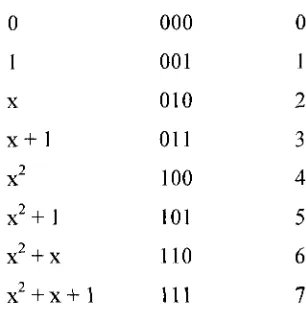
Consider GF(23) with Irreducible polynomial P(x) = x3 + x2 + 1. This field has 8

0

1

X

x + 1

x2

x2+ l

x2 + x

x2 + x + 1

000 001 010 Oil 100 101 110 111 0 1 2 3 4 5 6 7

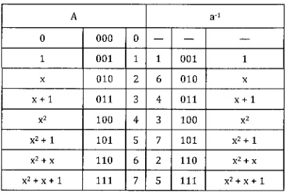
Addition and multiplication in this field is illustrated in the following tables:

0

1 X x + 1

X2

X2 + l

x2 + x

X2 + X + 1

000 0 0 1 010 O i l 100 101 110 111 0 000 0 1 001 1 010 2

x + 1 O i l

3

xz 100 4

x2 + l 101

5

X2 + X X2 + X + 1

110 111 6 7 0 1

0 2 3 0 3 2 1 0 4 5 6 7 0 5 4 7 6 1 0 6 7 4 5 2 3 0 7 6 5 4 3 2 1 0

Table 2.1 Addition in GF(23)

x2+ 1 X2 + X X2 + X + 1

X

000 0

001 010 O i l 100 101 110 111 0 000 0 1 0 0 1

1

010 2

x + 1 O i l 3

x2 100

4

Table 2.2 Multiplication in GF(23)

x2+ 1 1 0 1

5

X2 + X Xz + X + 1

110 111 6 7 0 0

A

0

1

X

x + 1

X2 x2 + l X2 + X

X2 + X + 1

000 001 010 Oil 100 101 110 111 0 1 2 3 4 5 6 7 a-1 — 1 6 4 3 7 2 5 — 001 010 Oil 100 101 110 111 — 1 X

X + 1

X2 x2 + l x2 + x X2 + X + 1

Table 2.3 Multiplicative Inverse Elements in GF(23)

2.6 Basis in Finite Fields

In the previous example we represented field elements as a polynomial of degree less

than or equal to 2. But there are other ways to represent the field elements. In general,

any element a of a finite field GF(2") can be represented as:

a = a0/?0 + a1/?1 + - + an_1/?n_1 (2.8)

where at 6 GF(1) and fa E GF(2") for 0 < i < n - 1

The set {/?», Pi, ..., /?„./} which contains n linear independent elements is the basis of the

field [23]. There are different types of basis for finite fields. Some of the most important

types are:

• Polynomial Basis

• Normal Basis [31]

• Dual Basis [25]

• Triangular Basis [11]

• Weakly Dual Basis [39]

• Redundant Representation [40]

In the previous example, elements of the finite field were represented in polynomial

basis. Here we give a brief review to polynomial basis. Some of the other bases are

discussed in the next chapter.

Polynomial Basis

Consider a finite field GF(2") with an irreducible polynomial f(x). If a be a root of this

irreducible polynomial, then the set {1, a, a2, ..., an"'} forms a polynomial basis. In

polynomial basis representation, any element a of the field is represented as:

n - l

a = an_1a11~1 + an_2an _ 2 H 1- ata + a0 — J atal

(2.9) 1 = 0

It should be noted that since we are not interested in evaluating a for a specific value of a,

other variable symbols can be used instead of a too. As you have mentioned in the

previous example we represented the elements of GF(23) as aix2 + ajx + ao, but by x we

mean the root of the irreducible polynomial.

2.7 Finite Field Multiplication in Polynomial Basis

Consider a Finite field GF(2") with the irreducible polynomial/*) as:

n - l

f(x) = x

+ Y

f

x

+ l

where/; E GF{2)

(2.10)

i = i

Consider a and b as two elements of this field. By employing polynomial basis we have:

n - l n - l

A(x) = y atxl and B(x) y btxl

The multiplication operation is then defined as:

n - 1

C(x) = A(x)B(x)modf(x) = V q x '

i=0

(2.12)

This operation is performed in two steps:

1. Polynomial multiplication

2. Reduction modulo irreducible polynomial

Step 1:

In this step A(x) is multiplied by B(x) resulting in D(x), considering the polynomial

multiplication rules mentioned in section (2.4):

2n-2

D(x) = A(x)B(x) = V dtx1

1 = 0

(2.13)

The coefficients ofD(x) are calculated as follows:

( _L

dt = {

y cijbi-j for 0 < i < n - 1

;'=0 n - l

2 ^ ajbi_j fc for n < i < 2n — 2

yj=i-n+l

This polynomial operation can be represented in a matrix form as:

(2.14)

Where D is the coefficient column vector of D(x), B is the coefficient column vector of

B(x), and M is the Multiplication Matrix which contains coefficients of A(x) with the

following form:

% - 2

n-l

d„

l*1„_->

a.

a n-l

0

0

0

0 0

an

a„ "*n-l

0 0 0 an 0 0 0 0 0 o0 a. a. 2. a? a„-i 0 0 " 0 0 0 a0 a. 1 a2 a„-2 an-\_ X

h

L" n~i _

(2.16)

Step 2

The result of the previous step was the polynomial Dfx) which obviously has a degree

bigger than n — 1. Therefore it needs reduction. By reduction, we want to reduce the

degree ofD(x) from 2n - 2 to n - 1. This reduction process is defined as follows:

C(x) = D(x)mod f(x)

n-l

= y dtxl mod f{x)

i=0

n-l n-2

(2.17)

y dtxl+y dk+nxk+n mod f(x)

! = 0 fe=0

It is clear from the above equation that the reduction step is only performed on the

elements of D(x) which have a power greater than n.

" x" '

x"+l

x2-3

_x2-2_

= Tx

V ~

n-2 X

X

1

(2.18)

k+n

Clearly the role of this matrix is to find the residue of each x ", for 0 < k < n-2, modulo

f(x).The entries of this matrix are either " 1 " or "0", and the form of this matrix directly

depends on the irreducible polynomial. As an example, consider finite field GF(25) with

the irreducible polynomial/^ = x5 + x2 + 1. Consider a as a root off(x). We have:

ab + a1 + 1 = 0 => a5 = a1 + 1 (2.19)

Note that since we are in finite field GF(2n), -a5 = a . Multiplying both sides of (2.19) by

a consequently, will result in:

(ab — as + a

la7 =

a

a

(a8 = a5 + a3 = a2 + 1 + a3

(2.20)

And matrix T is built as:

0 0 1 0 1

0 1 0 1 0

1 0 1 0 0

0 1 1 0 1

So by using (2.18) we can write:

x*+"mod/(x) = 5 X X "y

-7=0

And by substituting (2.21) in (2.17) we have:

n - l n - 2 n - 1

C(x) = ^ diX

+ ^ d

]T t^-J-

i=0 fe=0 ;'=0

n - l n - l n - 2 (2.22)

"•n+ktk,n-j-lx

i=0 ;'=0 k=0

Hence, the final result is calculated.

2.8 Multiplier Architecture and Complexity

Hardware realization of (2.16) and (2.22) leads us to an actual circuit which is capable of

performing finite filed multiplication. This circuit will receive coefficients of two

elements of the finite field, a and b, at the input and gives the coefficients of c at the

output. Since our finite field is of the form GF(2"), the operations on the coefficients are

performed in GF(2). Therefore the multiplication operation is realized as a 2-input AND

gate, while the addition operation is realized with a 2-input XOR gate.

In different hardware architectures for finite field multipliers, the important factor is to

minimize the complexities. By complexity we mean two things:

• Space Complexity

• Time Complexity

Space complexity is the total number of gates used in the hardware realization of the

multiplier. Since we just use two types of gates; i.e. 2-input AND gates, and 2-input XOR

gates, space complexity is expressed in terms of the total number of these two gates.

Time complexity is the actual delay of the circuit. In other words, if the two inputs a, b be

circuit is the delay of the gates used in circuit. Again, since we just have two types of

gates in the circuit, time complexity is expressed in terms of the delay of a 2-input AND

gate, TA, and the delay of a 2-input XOR gate, Tx.

When realizing the circuit for (2.16), due to the shape of matrix M we need n AND gates

and (n - 1)' XOR gates. All of the AND operations can be done in parallel so the total

delay of the AND gates would be one TA. The biggest XOR chain happens when

realizing (ao a; ... a„.i) (bob/ ... b„.i) . This operation needs n - 1 XOR gates. By using a

binary tree structure, the total delay of this operation would be \ l o g2« - l |. Space and

time complexity of realization of (2.22) directly depends on the form of the irreducible

3 An Overview of Finite Field Multipliers

In this chapter we give a brief overview of the state of the art research in the field of finite

field multiplication.

Finite field multipliers can be categorized based on their hardware architecture into three

types:

• Parallel Multipliers

• Serial Multipliers

• Hybrid Multipliers

Bit parallel (or full parallel) finite field multipliers are the main subject of this thesis. In

these multipliers, inputs and outputs are presented at the input ports in parallel at once.

The output of the multiplier is ready at the output port after some delay. But no clock

cycle is needed for performing multiplication operation.

On the other hand, bit serial multipliers receive the input bits in serial, and also perform

the multiplication operation serially. So the output will be ready after some clock cycles,

bit by bit. Hybrid multipliers can receive the inputs serially, but they may perform the

In this chapter we first thoroughly review the best bit parallel finite field multipliers.

Then we will briefly review some serial multiplier architectures.

3.1 Parallel Finite Field Multipliers

One of the most important contributions to this field of research is the work of Mastrovito

in [21]. In the previous chapter we showed the actual multiplication of two elements in a

finite field of form GF(2n) regarding the polynomial basis. That method is called

conventional multiplication and has two steps: the first step is multiplying two

polynomials and the second step is reducing the result of the polynomial multiplication

by the irreducible polynomial. On the other hand, Mastrovito has introduced another

method in [21] which has been called mastrovito multiplier in literature. Mastrovito

multiplier combines those two steps in just one matrix multiplication. The whole concept

of mastrovito multiplier is to find a matrix M (later called matrix Z) which satisfies the

following equation:

C = MB (3.1)

where

M =

J0,0 ' " J0,n-1

/ n - 1 , 0 ••" V n - l , n - l

(3.2)

The entries of matrix M depend on the coefficients ofA(x) and on the coefficients of the

T matrix as follows:

rat for v' = 0 and 0 < i < n — 1

l,J ' u(i — j)at^j + y tj_1_kian^1_k for 1 < j < n — 1 and 1 < i < n — 1

fe = 0

In the above formula u is a step function defined as:

u ( t )

= to t < o

-

It is important to note that although mastrovito multiplier is referred to as a one step

multiplication method considering the conventional two step method, but it also has two

steps itself. The first step is to build up the M matrix, and the second step is to perform

the matrix multiplication. Mastrovito multiplier has been used as the base of many

efficient finite field multiplication methods since it was presented.

Another important contribution in this field was the work of Paar in [27]. Paar combined

the conventional multiplier with Karatsuba-Ofman algorithm (KOA) in order to gain

more reductions in space complexity. KOA was first introduced in [14] as a method for

multiplying large integers. KOA is a divide and conquer form algorithm that divides the

operands into two parts with less number of digits (half number of digits) and forms the

final result with the help of the product of these parts. A good explanation of KOA

algorithm can be found in [15]. This idea can directly be applied on polynomial basis

representation of finite fields since each element can be represented by the coefficients

which are in the field of GF(2); i.e. {0,1}. Therefore the representation of the field's

elements would be a string of bits.

Regarding the conventional method of multiplication, KOA is a method for improving

the first step. Applying KOA to polynomial multiplication would be recursive if the

degree of the polynomials is n - 1 and n is a power of 2. Let's consider two elements a

and b in a finite field GF(2n):

A(x) = an^xxn~1 + —I- atx + a0

B(x) = bn^x71'1 + --- + b1x + b0

- / - - 1 \ / - - 1 \

-A(x) = x2 I an_1x2 H h am\ I + I a<n_\x2 +—\-atx + a0\ — x2AH + AL

— I —-1 \ / —-1 \ 21 B(x) = X2 \bn_xX2 + ••• + brn\ J + \btn_ NX2 + ••• + fc1X + fe0J = X 2 SH + SL

(3.5)

Therefore with this new notation, we can change the method of multiplying those two

polynomials, from the conventional multiplication method, which involves multiplying

each element in A(x) to all the elements in B(x), to a new method as below:

A(x)B(x) = (xn2AH + AL) (xn2BH + BL)

(3-6) = xnAHBH + X2{(AH + AL)(BH + BL) - (AHBH + ALBL)} + ALBL

It is obvious that subtraction in the second term is the same as addition since we are using

the fields of characteristic 2. The gate complexities for conventional method as

mentioned in chapter 2 are:

(#AND=n2

\#XOR= ( n - 1 )2 ( '

But the corresponding complexities for the new method are:

#AND = -n2

3 (3-8)

l#XOR = - n 2 + n - l

4

Further reductions can be gained by applying the same method on the polynomial

multiplications: AHBH, Ajfiu a nd (AH + AL)(BH + BL). It is obvious that this procedure of

splitting polynomials can be applied recursively in i steps, where /' = log2 n. It has been

mentioned in [27] that the total space complexity would be:

The method of Parr in [27] was widely used later for building sub-quadratic space

complexity multipliers.

Fenn et al presented a parallel dual basis finite field multiplier in [8]. First we have to

define dual basis: A set of n elements {/?«, Pi, ..., /?„_/} forms a basis for GF(2") if the PJS

are linearly independent over the field GF(2). Letf(x) be an irreducible polynomial of

degree n, then as we mentioned in chapter 2, the polynomial basis of the field would be

{], a, a2, ..., a"'1}, considering a as a root offfx). The trace of /? G GF(2n) relative to the

subfield GF(2) is defined as:

n - l

7 Y ( / ? ) = ^ / ?2 i

(3.10) 1=0

This trace function is a linear mapping from the finite field GF(2") onto the finite field

GF(2). Let {a0, a/, ..., an-i} and {/?& Pi, .... /?«./} be any two bases for GF(2n) and also let

Y 6 GF(2n) with y ^ 0. Then these two bases are said to be dual with respect to y if:

Tf y is a fixed non-zero element of the field, and if {p0, Pi, ..., pn-i) is a dual basis of the

polynomial basis, {1, a, a2, ..., a"'1}, then

polynomial basis or dual basis as follows:

polynomial basis, {1, a, a2, ..., a"'1}, then any element a of the field can be expressed as

n-X n - l

j=o i=o (3.12)

In order to find aj*s we use (3.11):

n - l \ n - l

Tr(

aU) = Tr

a

] T a*ft = £ a\Tr{ya^i) = a*

i=o / i=o

Now consider two elements a, b in the field. We want to find c = a x b mod/fx). Here a

is represented over dual basis and b is represented over polynomial basis as:

n - l

i=o

n - l

V

bi a

b

(3.14)

Then c can be obtained as follows:

<x, a,

a. a.,

tf„ i a„

a n-l *

<2„ _(3.15)

In the above formula a\s for n<i< 2n-2 are recursively calculated as follows:

n - l

*n+fc / a fjaj+k

;=0

/ o r 0 < fc < n - 2

(3.16)

In which, j^s are the coefficients of the irreducible polynomial of the field. From (3.15)

we have:

c0 = a*0b0 + a{bx + ••• + c d ^ . i

c1 = alb0 + a*2bx + — h a*nbn_t

<cn-l = an-1^0 + an ^ l + l~ a2n-2^n-l

(3.17)

From the above equations it can be seen that the n product bits are generated by n

identical functions of the form:

h(a, b) = a*kb0 + a*^^ + ••• + a ^ ^ ^

Therefore a bit-parallel dual basis multiplier for GF(2") can be constructed out of n GF(2)

inner product modules that implement (3.18), and one other module that generates the

an+k for 0 <k< n-2 from (3.16).

Koc and Sunar presented two new finite field multipliers for all one polynomials (AOP)

in [17]. The first multiplier was a polynomial basis multiplier based on the mastrovito

multiplier with a slight change, and the second one was a normal basis multiplier.

An AOP over the finite field of GF(2") is a degree-n polynomial with all the coefficients

as 1; \.Q.f(x) = x" + x n-l + x + 1. According to (3.2) and (3.3) the mastrovito matrix

of an AOP of degree n would be as follows:

an-i

an + a„

an-t+a„_2 an_2+an_3

*n-2 «„-l+«„-3

an_2 a^ + a^ an_4 + an_2 an_5+a,^

«„_! « „ - 2 + " „ - l a„ - 3 + « „ - 2 a„

a2 +a{

o, +a.

an + a.

(3.19)

This matrix can be decomposed into matrices Z\ and Z2 as Z = Zi + Z2:

a0

« i

°n-2

-Qn-\

0

a0

a„ -3

an-2

an-\

0

a„-4

an-3

an-2 •

a„-\ •

an-5 •

«„-4 '

•• a2

•• a.

•• 0

• v

Z2 =

"0 0 0 0 «„-! °n-\

an-\

an->

a„-2 a„-2

an-2

a„-2

a„-3 •

an-3 •

a»-3 •

an-3 •

•• a .

•• a.

• • a\

• a ,

(3.20)

Now in order to compute C = ZB = (Z] +Z2)B, first we compute D = ZiB and E = Z2B in

parallel, and then we compute the result C = D + E. By using this method, time delay of

Before reviewing the second multiplier presented in [17] we have to explain normal

basis. A set N of the form N = {^yS2,/?22,---,/?2""1} in a finite field GF(2") forms a

normal basis, where /? is the root of the irreducible polynomial. Since the irreducible

polynomial of the field is an AOP we have:

Pn+X = 1 (3.21)

Further more if 2 is primitive in Zn+i then we have:

N = {fi,p

,p

,-,p

} (3.22)

Set N in (3.22) is also a basis. It is actually a shifted version of the polynomial basis. Any

element a of GF(2") represented with normal basis can easily be converted to this shifted

polynomial basis (SPB) representation as follows:

n - l n - 1

i=0 i=0

(3.23)

The coefficients of the shifted polynomial basis can be obtained as:

S w(n+i ) = ^ f°r 0<i<n-l (3.24)

In this multiplier, the two inputs a and b are first converted from normal basis to shifted

polynomial basis, then a regular polynomial basis multiplication is performed. At the end

of this computation the result is obtained as g = ab/p~:

g= gn-iPn~1+ -+ giP + g0

= (dn_i + e)/?""1 + - + (dj + e)P + (d0 + e) (3.25)

Note that dk = Z,(k, :)B for 0 < k < n - 1 and e = Z2(0, :)B = Z2(l, :)B = ... = Z2(n-1, :)B,

Then we have to multiply g by /? :

h = (dn_i + e)/?n + 1 + (dn_2 + e)(ln + •••+ (d± + e)/?3 + (d0 + e) /?2 (3.26)

Since / ?n + 1 = /? + /?2 + ••• + /?n, the coefficient (</„./ + e) is added to all the other

coefficients. Therefore we can write h in shifted polynomial basis as:

h = (dn_2 + dn^Wn + - + (dj + dn.t)p3 + (d0 + dn_ 0 /?2 + (dn_! + e)/? (3.27)

In order to convert h in SPB to the final result, c, in normal basis we just apply the

reverse of (3.23).

When mastrovito multiplier was introduced in [21], it was only analyzed for trinomials of

type x" + x + 1. The space complexity of this multiplier was: n2 AND gates, and n2 - 1

XOR gates. Sunar and Koc presented a new formulation of the multiplication matrix in

[37]. With the help of this formulation, new multiplier architecture was presented for

mastrovito multiplier, in which the XOR complexity was n2 - 1 for all trinomials of type

x" + x' + 1 for 0 < t < n and rf ^ 2t. Furthermore it was proved that if n = 2t, then the

XOR complexity would be n - n/2.

As we explained in chapter 2, in a finite field GF(2") with f(x) as the irreducible

polynomial in polynomial basis, in order to find c = ab mod f(x) we first find d = ab;

D(x) is a polynomial of degree 2n - 2. Tn the next step Dfx) is reduced by thef(x) to C(x)

which is a polynomial of degree n - 1. Matrix representation of the first step as described

d.

" n - 2 d„-l

d„ d. n+\

*2n-2. 0 0 0 0 0 0 0 0 "*H-4 0 0 0 0 0 a0 at a2 a. a, 0 0 0 0 a0 a, a.

n-\ an-2

K-2

It is important to note that, not all the elements of d need reduction in the second step, but

only the elements of d that have a power of x bigger than n - 1. The number of reductions

for a specific element depends on the degree of the element and on the value of the

middle term of the irreducible trinomial; i.e. /. The maximum number of reductions is

performed on the highest order element d2„-2- Let k be the number of reductions required

for this element. This integer k has the property 2n - 2 - k(n - t) < n, which implies

k > . Therefore, we have:

n-t '

n-2

n-t + 1 (3.28)

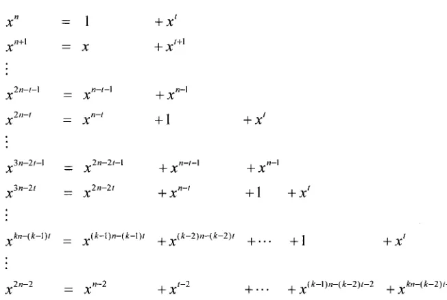
The objective of [37] is to obtain the matrix Zn x n by systematically reducing the last

n - 1 rows of the matrix M(2n-i) x n using a general trinomial. In order to accomplish this

x" = 1

x"+l = x _{+ x"}

2n-t-\ n-l-i X = X

+ x

x3"-2' = x2"-2' +X-1 _{+ 1 +x'}

*n-(*-l)< _ x(k-\)n-(k-\)l (A-2)n-(*-2)< +, , _ + 1

+ X

K - 2 .1-2 _| + <*-l)n-(*-2)'-2 + *»-(*-2)(-2

X + X '

Figure 3.1 Reduction Array for a General Trinomial

The columns of the reduction array have the following properties:

The first column on the right-hand side is the sequence 1, x, x2, ..., x"'1;

n-l

The second column contains two sequences: The sequence x, x'+l, ..., x

followed by the sequence 1, ..., x"'''1, x"~', ..., x"'2;

For 3 <i < n-l, the i'th column is obtained by shifting down the (i - l)'th column

m-t positions;

It is also seen that the reduction array can be divided into k partitions, and each partition

has n-t terms except for the last partition which may have less terms. Tf the partitions are

enumerated in increasing order, beginning from the topmost as the Oth partition, the i'th

partition will consist of the rows starting with the term x"^"'^ and ending with the term

n+(i+l)(m-t)-l

In the reduction process the rows defined by the reduction array are added to the rows of

matrix M in order to eliminate the last n-l rows of M. The exponent on the left-hand

side provides the index to the source row, and the exponents on the right-hand side

In order to construct the Z matrix the following formulation is used:

Z = X + Y (3.29)

Where matrix X is the upper n rows of matrix M (destination rows) and matrix Y is the

contribution of the n- 1 lower rows of matrix M (source rows):

X =

ao

ai

a2

an-2

_an-X

0

a0

« i

a„-3 an-2

0 •

0 •

a0 •

a„-A •

an-3 •

•• 0 •• 0 •• 0

•• a0

• a . 0 0 0 0 a0 (3.30)

Since we have two types of sequences on the right hand side columns: those of form

1, x, x, ...,x"~~ or 1,..., x"''~J, x"~', ..., x'2, and those of form x', x'+l, ...,xn~', we can write:

Y = T + U (3.31)

Where T is the contribution of the first type of sequences, and U is the contribution of the

second type of sequences. The first column is the sequence 1, x, x2, ...,x"~2. So we have to

add the rows M(n, :), M(n+1, :), ..., M(2n-2, :) to Z(0, :), Z(l, :), ..., Z(n-2, :). This

contribution of the first column is shown in the matrix below:

T = "0 0 0 0 0 «m-,

0

0

0

0

am-i •

<*m-\ •

0 •

0 •

0

a2

•• a3

•• am_x

The second sequence in the second column is 1, ..., x"~'~, x"'1, ..., x1'2. So we add the rows

M(2n-t, :), M(2n-t+l, :), ..., M(2n-2, :) to Z(0, :), Z(l, :), ..., Z(t-2, :). This can be shown

by shifting up matrix To n -1 rows: Ti = To[|(n-t)]. By similarity we have:

T

= T

_

[Hn-t)]=T

[U(n-t)]

fc-1

T = T0 + T1 + - + Tk_± = ] T T0 [T i(n - t)]

(3.33)

i = 0

The first sequence in the second column is the sequence x, x'+l, ...,xn']. So we have to add

the rows M(n, :), M(n+1, :), ..., M(2n-2, :) to the rows Z(t, :), Z(t+1, :), ..., Z(n-1, :).

This is done with the help of matrix UQ:

U0 =

0 0 0

0 0 0

0 0 a.,

0 0 0 0

0 0

0 0

a, a.

CY^ C » T

t-\ t t + \

n-\

(3.34)

The first sequence in the third column is x', xt+l, ...,xn~''. So we add the rows M(2n-t, :),

M(2n-t+l, :), ..., M(2n-2, :) to the rows Z(t, :), Z(t+1, :), ..., Z(n-1, :). This can be shown

by shifting right matrix Uo n -1 columns: Ui = Uo[—*(n-t)]. By similarity we have:

Ui = U i - i h in - t)] - f /0h Kn - t)]

fc-i

U = U0 + U1 + - + l/k_! = ^ U0 [-> i(n - t)]

(3.35)

1 = 0

Z = X + Y

=X+T+U (3.36)

fc-1 fc-1

= X + £ 70 [T i(n - t)] + ^ "o [-» i(n - 0 ]

i=o i=o

Mastrovito multiplier did not show promising results for finite fields defined by high

hamming weight (the number of nonzero coefficients) irreducible polynomials. As a

solution, Song and Parhi presented a modified mastrovito multiplier in [36]. With this

architecture, it is possible to build finite field multipliers for GF(2") with XOR

complexity proportional to n — 1 - pwt, in which pwt is the hamming weight of the

irreducible polynomial.

Tn order to compute c = ab in finite field GF(2n) with modified mastrovito multiplier, first

a modified mastrovito matrix U is built and D = UB is computed as follows:

TT R —

,0 n-\ 0

• • « " " , ' "

n-\

•• Un-2

- <~X

•• u"_;1

' K"

K\

X,"

dn-7

d0 . < _

= D (3.37)

The coefficients of matrix U are calculated as follows:

ru° — a

o

u \

U - i = i ^ - i

for 0 < i < n - 1

/ o r 0 < i , k<n — 1 (3.38)

/ o r 0 < ik < n - 1

whereas are the coefficients of the irreducible polynomial. Then c = ab can be obtained

dn_x+dc

dn_2 + dc

d0 + dc

(3.39)

Detailed proof of (3.39) can be found in [36].

Following the work of Sunar and Koc in [37], Halbutogullari and Koc tried to find a

general formulation for mastrovito multiplier with any type of irreducible polynomial in

[9]. Although this formulation covers all the polynomials of the form:

fix) = xnk + x"*-1 + ••• + xni + xn°

where n = nk > tin > ... > ni > no = 0, but it does not offer a practical way of hardware

implementation of the multiplier. However it analyzes the mastrovito multiplier for an

equally spaced polynomial (ESP) and shows very promising complexities for this type of

irreducible polynomials. In a finite field GF(2n) an irreducible ESP has the following

form:

/ ( * ) = *** + x(*-i)A + -..+ 1 (3.40)

where kA = n. the space complexity of the mastrovito multiplier for such polynomial

would be:

(#AND = n2

UXOR = n

- A

(3.41)

A special case of ESP is the trinomial of the form xn + x~z + 1. The complexity of XOR

gates for a multiplier with this polynomial would be #XOR = n" — n/2. To the best of our

knowledge, so far this is the lowest complexity of a finite field multiplier in literature. It

has been proved in [9] that a mastrovito multiplier cannot have space complexity better

(#AND = n2

{#XOR=n*-\ (

'

)

Although [9] provided a general formulation for mastrovito multiplier, a systematic

method of designing this multiplier was not available until Zhang and Parhi presented an

explicit algorithm for efficiently designing that in [41].

Considering finite field GF(2n) with a general irreducible polynomial f(x) we have:

7(x) = x

+ A*""

+ - + A* + /„

J ft G {0,1} for 0 < i < n - 1 (3.43) J o = l

(3.43) can also be written as:

(f(x) = xn + xks + x^-1 + ••• + xkl + 1

[ n> ks> fcs_j > ••• > kt > 1

(3.44)

Now a set N can be built with the following algorithm from [41 ]:

Input: The parameters of irreducible polynomial: n, k/, ..., ks

Output: set N c {0,1, • • • , « - 2} Procedure:

Step 1: Generate a weighted tree D according to the following properties:

• Each node dj in D has at most s child nodes and each edge has the weight WG{(n-k,)\\<i<s}

• Let dj denote the root andh(dj, dj denote the weight of path from d/ to dj, where h(dj, d/) = 0; for all djS, if 3r e {{n — kl. | 1 < / < s} and