First Principles Investigation of Technologically and Environmentally Important Nano-Structured Materials and Devices

ABSTRACT

PAUL, SUJATA. First Principles Investigation of Technologically and Environmentally Important Nano-structured Materials and Devices. (Under the direction of Marco Buongiorno Nardelli).

In the course of my PhD I have worked on a broad range of problems using simulations from first principles: from catalysis and chemical reactions at surfaces and on nanostructures, characterization of carbon-based systems and devices, and surface and interface physics. My research activities focused on the application of ab-initio electronic structure techniques to the theoretical study of important aspects of the physics and chemistry of materials for energy and environmental applications and nano-electronic devices. A common theme of my research is the computational study of chemical reactions of environmentally important molecules (CO, CO2) using high performance simulations. In particular, my principal aim was to design novel nano-structured functional catalytic surfaces and interfaces for environmentally relevant remediation and recycling reactions, with particular attention to the management of carbon dioxide.

the carbon-mediated partial sequestration and selective oxidation of CO in a hydrogen atmosphere.

We have elucidated the atomic scale mechanisms of activation and reduction of carbon dioxide on specifically designed catalytic surfaces via the rational manipulation of the surface properties that can be achieved by combining transition metal thin films on oxide substrates. We have analyzed the mechanisms of the molecular reactions on the class of catalytic surfaces so designed in an effort to optimize materials parameters in the search of optimal catalytic materials. All these studies are likely to bring new perspectives and substantial advancement in the field of high-performance simulations in catalysis and the characterization of nanostructures for energy and environmental applications.

Moving to novel materials for electronics applications, I have studied the structural and vibrational properties of mono and bi-layer graphene. I have characterized the lattice thermal conductivity of ideal monolayer and bi-layer graphene, demonstrating that their behavior is similar to that observed in graphite and indicating that the intra-layer coupling does not affect significantly the thermal conductance. I have also calculated the electron-phonon interaction in monolayer graphene and obtained electron scattering rates associated with all phonon modes and the intrinsic resistivity/mobility of monolayer graphene is estimated as a function of temperature.

On another project, I have worked on ab initio molecular dynamic studies of novel Phase Change Materials (PCM) for memory and 3D-integration.

an engineering transport model of the component electrochemical cell. To support that model, we have proposed a reaction kinetics expression for the REDOX (reduction-oxidation) reaction at the porous positive electrode. We validate the kinetics expression with electrochemical measurements.

First Principles Investigations of Technologically and Environmentally Important Nano-structured Materials and Devices

by Sujata Paul

A dissertation submitted to the Graduate Faculty of North Carolina State University

in partial fulfillment of the requirements for the degree of

Doctor of Philosophy

Physics

Raleigh, North Carolina 2010

APPROVED BY:

_______________________________ _____________________________

Jerry Bernholc Lubos Mitas

________________________________ ______________________________

Thomas P. Pearl Gregory Parsons

DEDICATION

BIOGRAPHY

Education

2005 - 2010: PhD in Physics, Department of Physics, North Carolina State University, Raleigh, NC 27695, USA

2000 – 2003: Senior Research Fellow (SRF) at S. N. Bose National Center for Basic Sciences, Kolkata, India

1998 – 2000: MSc in Physics (Specialization: Electronics) at Kalyani University, West Bengal, India

1995 – 1998: BSc in Physics at Kalyani University, West Bengal, India

Professional Experience

May - August 2009: Summer Intern @ IBM SRDC, Albany Nanotech, Albany, NY May - August 2008: Summer Intern @ Polymer and Chemical Technologies Division, General Electric Global Research Center, GE, Niskayuna, NY

ACKNOWLEDGMENTS

I would like to acknowledge my advisor Prof. Marco Boungiorno Nardelli for his constant support and encouragement throughout the course of my stay in North Carolina State University. I would also like to thank my committee members for taking time out of their busy schedules to critique this work.

I had an opportunity to do three industrial internships at IBM and General Electric during my tenure as a PhD student. I had the good fortune of participating in vibrant research projects at these corporate research labs in areas as diverse as Phase Change memories, electrochemistry and advanced device design for 15 nm technology nodes. For this, I’d like to acknowledge Dr. Glen J Martyna (IBM), Dr. Michael Vallance (GE), Dr. Glen Merfeld (GE) and Dr. Huiming Bu (IBM) for mentoring my progress during the summers of 2007, 2008 and 2009.

I would like to thank my parents and my husband, Kingsuk Maitra for helping me reaching my goal; friends and near ones like Nancy, Frisco, Jeff, and Cecillia made my stay at North Carolina a very memorable one. Nancy and Cecillia were always there when I needed them most.

My adopted family members at North Carolina Jill and Alan (and their siblings) offered me a home far away from home. Thank you Jill.

TABLE OF CONTENTS

List of Tables...x

List of Figures ...xi

Chapter 1 ...1

1.1 Introduction...1

1.2 Density Functional Theory (DFT)...3

1.2.1 Exchange and correlation functional for DFT... 8

1.2.2 Plane wave basis set ...10

1.2.3 Pseudopotential ...11

1.2.4 Computation with DFT ...13

1.3 Post-Processing: Tools and Capabilities...16

1.4 Nudged Elastic Band Method (NEB)... 20

1.5 Density Functional Perturbation Theory (DFPT)...22

1.6 Ab Initio Molecular Dynamics (AIMD)...25

1.7 Partition Functions of Molecules and Solids (ParFuMS)...28

1.8 Organization of The Thesis...29

Figures...32

References...37

Chapter 2: Sequestration and selective oxidation of carbon monoxide on graphene edges...40

2.1 Introduction...40

2.2 Methods...42

2.3 Results and Discussion...44

2.3.2 Interaction of CO with armchair graphene edge ...48

2.3.3 Interaction of CO+H2 with armchair graphene edge ...52

2.4 Concluding Remarks...55

Figures...57

References...68

Chapter 3: Activation of CO2 on transition metal surfaces and oxide supported metal thin films... ...70

3.1 Introduction...70

3.2 Computational details...75

3.3 Theoretical results...78

3.3.1 Activation of CO2 on Pd (001)...78

3.3.2 Activation of CO2 on Pt (001)...81

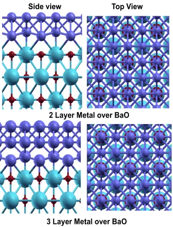
3.3.3 Oxide Supported metal thin film...83

3.3.4 Activation of CO2 on 1LPd/BaO (001)...84

3.3.5 Activation of CO2 on 1LPt/BaO (001)...89

3.3.6 Activation of CO2 on 2LPd/BaO (001) and 2L Pt/BaO(001)...92

3.3.7 Activation of CO2 on 3LPd/BaO (001) and 3L Pt/BaO (001)...94

3.4 Conclusion...96

Tables...96

Figures...102

References...134

Chapter 4: First principles calculations of structural, vibrational properties of mono and bi-layer graphene...135

4.2 Computational Details...136

4.3 Band structure...137

4.4 Phonon dispersions...139

4.5 Electron phonon interaction...141

4.5 Conclusion...142

Figures...143

References...151

Chapter 5: Ab initio molecular dynamic studies of Novel Phase Change Materials for memory and 3D-integration ...153

5.1 Introduction...153

5.2 Methods...158

5.3 Liquid GST systems...160

5.3.1 Liquid Ge0.15Te0.85: The Eutectic Alloy ...160

5.3.2 Liquid GeTe ...161

5.3.3 Liquid Ge1Sb2Te4...161

5.4 Pressure induced transformation of Ge2Sb2Te5...162

5.5 Pressure induced transformation of GeSb...163

5.6 Conclusion...165

Figures...166

References...181

Chapter 6: Na / NiCl2 Cell Positive Electrode REDOX Kinetics: Model development and verification ...183

6.1 Introduction...183

6.2 Previous models of Sodium/metal chloride cells...185

6.3.1 Oxidation...187

6.3.2 Reduction... 191

6.3.3 Relationship between NiCl2 volume fraction and passivation area density during oxidation... ...193

6.3.3.1 Homogeneous, invariant oxidation...194

6.3.4 Relationship between NiCl2 volume fraction and passivation area density during reduction... ...195

6.3.4.1 Homogeneous, Invariant Reduction...196

6.3.5 Verification of Kinetics Model with Smooth Electrode REDOX ...197

6.3.5.1 Oxidation... ...197

6.3.5.2 Reduction... ...199

6.4 Materials and Electrochemical Methods...201

6.4.1 Working Electrode... ...201

6.4.2 Reference Electrode... ...202

6.4.3 Auxiliary Electrode... ...202

6.4.4 Electrolyte... ...202

6.4.5 Electrochemical characterization...202

6.5 Results and Analysis...205

6.5.1 Electrochemical Data... ...205

6.5.2 Finite Element Analysis (FEM).... ... 206

6.5.3 Oxidative Charge Capacity... ...210

6.5.4 Verification of Kinetic Model... ...212

6.6 Conclusion...214

List of symbols...215

References...219

Chapter 7: Extraction of effective oxide thickness for SOI FINFETs with

high-κ/metal gates using the body effect ...234

7.1 Introduction ...234

7.2 Theory and experiment...238

7.3 Discussion ...242

Figures...244

References...252

Chapter 8: Summary... ...254

Summary...254

LIST OF TABLES

Chapter 3: Activation of CO2 on transition metal surfaces and oxide

supported metal thin films......70

LIST OF FIGURES

Chapter 1: Introduction

Figure 1.1 Modeling a physical phenomenon from a broad range of

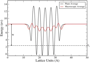
perspectives, from the atomistic to the macroscopic end ...32 Figure 1.2 Plane average and macroscopic average of 5 layer Pt (001) Surface ...33

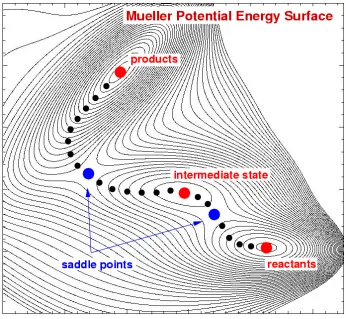
Figure 1.3 Activation energy barrier (EA), saddle point in a chemical reaction. ...34 Figure 1.4 Potential energy surface, minimum energy path is depicted along

with the saddle point (transition state) between reactants and products of a chemical reaction ...35 Figure 1.5 Car-Parrinello Molecular Dynamics algorithm ...36

Chapter 2: Sequestration and selective oxidation of carbon monoxide on graphene edges

Figure 2.1 Equilibrium energetics for a zigzag graphene edge interacting with CO molecules at high CO concentration ...57

Figure 2.2 Activation energy barrier for the reaction of an oxygen atom with CO to yield CO2 at the zigzag graphene edge...58

Figure 2.3 Activation energy barrier for the reaction of an oxygen atom with CO to yield CO2 when the oxygen atoms are bonded to 7-5-7 carbon rings at the zigzag graphene edge ...59

Figure 2.5 Energetics for the interaction of an armchair graphene edge with gas phase CO molecules. Table II (inset): the reactions at different steps and the corresponding reaction energies in kcal/mol...61

Figure 2.6 Activation energy barrier for the reaction of an oxygen atom with CO to yield CO2 at the armchair graphene edge ...62

Figure 2.7 Van’t Hoff plot for the two main steps in the deposition of carbon on an armchair graphene edge in a CO atmosphere ...63

Figure 2.8 Energetics for the competition between CO and hydrogen for the active sites on the advancing graphene edge ...64

Figure 2.9 Plots of equilibrium constants vs temperature for the main reactions In Figure 2.8...65

Figure 2.10 Representative chemical reactions of CO and H2 at the armchair graphene edge involving hydroxyl and carboxyl groups...66

Figure 2.11 Van’t Hoff plot for the reactions involving hydroxyl and carboxyl groups at the armchair graphene edge...67

Chapter 3: Activation of CO2 on transition metal surfaces and oxide supported

metal thin films

Figure 3.1 Adsorption geometries of CO2 on different sites of Pd (001) Surface ...102

Figure 3.2 Relative energy diagram of “CO2 dissociation” of Pd (001) Surface ...103

Figure 3.3 Surface LDOS of Pd (001) with adsorbed CO2 at different sites ...104

Figure 3.6 Adsorption geometries of CO2 on different sites of Pt (001) surface... ...107 Figure 3.7 Relative energy diagram of “CO2 dissociation” of Pt (001)

surface... ...108 Figure 3.8 Surface LDOS of Pt (001) with adsorbed CO2 at different sites ... ...109

Figure 3.9 LDOS of CO2 on Pt (001) surfaces...110 Figure 3.10 The charge density difference plot of “adsorptions of CO2 on Pt (001) surface... ...111 Figure 3.11 Barium oxide supported metal thin films: site A is supported over O atom and Site B is supported over Ba ...112

Figure 3.12 Activation of CO2 on 1LPd/BaO (001) surface...113 Figure 3.13 (a) Relative energy diagram of “CO2 dissociation” on 1LPd/BaO (001) surface... ...114 (b) Optimized structures of dissociation: the energetics are given in Figure 3.13(a)... ...115 Figure 3.14 Surface LDOS of 1LPd/BaO (001) with adsorbed CO2 at different sites... ...116

Figure 3.15 LDOS of CO2 on 1LPd/BaO (001) ...117 Figure 3.16 Adsorption geometries of CO2 on different sites of Pt (001) surface... ...118

Figure 3.19 Surface LDOS of 1LPt/BaO (001) with adsorbed CO2 at different

sites... ...122

Figure 3.20 LDOS of CO2 on 1LPt/BaO (001) ...123

Figure 3.21 The charge density difference plot of “adsorptions of CO2 on 1LPt/BaO (001) surface “...124

Figure 3.22 Barium oxide supported metal thin films...125

Figure 3.23 Activation of CO2 on 2LPd/BaO (001) surface...126

Figure 3.24 Activation of CO2 on 2LPt/BaO (001) surface...127

Figure 3.25 Activation of CO2 on 3LPd/BaO (001) surface...128

Figure 3.26 Activation of CO2 on 3LPt/BaO (001) surface...129

Figure 3.27 Binding energies of CO2 on different surfaces of Pd and Pd/BaO. ...130

Figure 3.28 Binding energies of CO2 on different surfaces of Pt and Pt/BaO ...131

Figure 3.29 Dissociation energy of CO2 [CO2 ⇔ CO + O] on different surfaces. Chemisorption energy at top site is considered as reference to calculate to dissociation energy...132

Figure 3.30 Dissociation of CO2 to CO and O atom over 2LMetal/BaO and 3LMetal/BaO. The dissociation energies are plotted in Figure 3.29...133

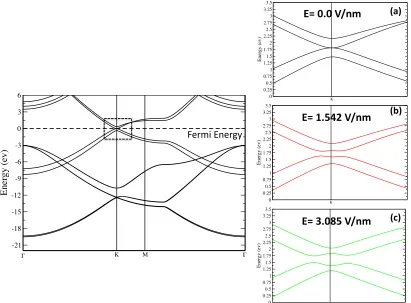
Figure 4.2 Left panel: electronic band structure of bi-layer graphene in the Along ΓKMΓ direction of Brillouin zone. Right panel: (a) band structure at zero gate field (b) band gap energy for the same system for an electric field with a potential energy U=0.5 V and (c) with potential energy U=1.0 V ...144

Figure 4.3 Phonon dispersion of monolayer graphene along the high Symmetry direction. Following the convention, the symbol Z denotes the out of plane vibration...145

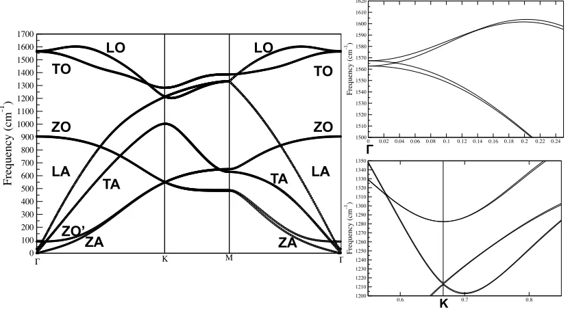
Figure 4.4 Left panel: phonon dispersion of bilayer graphene with A-B stacking along the high-symmetry directions. Following the convention, the symbol Z denotes the out of plane vibration; Right Panel: optical phonon dispersion near Γ and near Κ

...146 Figure 4.5 Effect of bias on the phonon modes (at K points) of monolayer graphene...147

Figure 4.6 Phonon density of states for monolayer graphene ...148 Figure 4.7 Electron phonon spectral (Eliashberg Function) function for monolayer graphene...149

Figure 4.8 Phonon linewidth for monolayer graphene ...150

Chapter 5: Ab initio molecular dynamic studies of Novel Phase Change Materials for memory and 3D-integration

Figure 5.1 The operation principle of a memory device based on phase changes ...166

Figure 5.3 Fragments of the local structure of GST around Ge atoms in the crystalline (left) and amorphous (right) state ...168

Figure 5.4 Total g(r) of Ge0.15Te0.85 calculated at T=943 K with 20ps

production run (left panel) is compared with the total g(r) calculated by Bichara et.al. [14] is given in the (right panel)...169

Figure 5.5 Experimental (right ) and calculated (left) total Structure factor at T=943K of Ge0.15Te0.85...170

Figure 5.6 Calculated pair correlation function g(r) at T=1000 K (left) and experimental g(r) of GeTe...171

Figure 5.7 Calculated structure factor S(q) at T=1000 K (left) and experimental S(q) (right) of GeTe liquid ...172 Figure 5.8 Calculated total pair correlation function at T= 973 K (left) for Ge1Sb2Te4 in comparison to experimental g(r) (right: blue curve) ...173

Figure 5.9 Calculated partial pair correlation function (left) for Ge1Sb2Te4. Partial pair correlation function calculated at ρ = 0.0297 Å3

(black curve) in reference [19] ...174 Figure 5.10 Calculated (left) and Experimental (right: blue curve) total Structure factor S(q) at T=973 K for Ge1Sb2Te4...175 Figure 5.11 Pressure induced transformation of Ge2Sb2Te5 : crystal to

Amorphous ...176 Figure 5.12 Total energy of 225 GST system with total run time of MD

Figure 5.15 A comparison of experimental and simulation structure factors for

amorphous phase ...180

Chapter 6: Na / NiCl2 Cell Positive Electrode REDOX Kinetics: Model development and verification Figure 6.1 Idealized geometry of the electrode...221

Figure 6.2 Cell Schematic...221

Figure 6.3 Chronopotentiographs for oxidation at T=300°C ...222

Figure 6.4 Chronopotentiographs for oxidation at T=325°C ...222

Figure 6.5 Chronopotentiographs for oxidation at T=350°C ...223

Figure 6.6 Chronopotentiographs for reduction at T=300°C...223

Figure 6.7 Chronopotentiographs for reduction at T=325°C...224

Figure 6.8 Chronopotentiographs for reduction at T=350°C...224

Figure 6.9 FEM Model of Cell...225

Figure 6.10 FEM Analysis for I = -0.009 A and tcf = 3.82 s. Left panel is electrolyte potential. Right panel is chloride ion concentration normalized by equilibrium concentration. ...225

Figure 6.11 Chloride ion concentration predictions at T=300°C versus reduced time at current densities 3.35 (oxidation) and –3.35 (reduction) A/m2. Terminal oxidation and reduction times were 1708.3s And 163.6 s, respectively...226

Figure 6.12 Effective resistance in equation 5.8. ...226

Figure 6.13 ΔU corresponding to a typical discharge chronopotentiograph (300°C, -0.0005 A) ...227

Figure 6.15 Parameters for equation 5.10 ...229

Figure 6.16 Linear relationship between ia (|ic|) and _η ...229

Figure 6.17 Comparison of predicted _η to measurement at T=300°C...230

Figure 6.18 Comparison of predicted η to measurement at T=325°C... 231

Figure 6.19 Comparison of predicted _η to measurement at T=350°C...232

Figure 6.20 Model parameters as functions of temperature ...233

Chapter 7: Extraction of effective oxide thickness for SOI FINFETs with high κ/metal gates using the body effect Figure 7.1 (a) A bulk planar MOSFET (b) Double gate SOI (silicon on insulator) MOSFET ...244

Figure 7.2 Cross section of FINFET. The fin is connected to source and drain. ...244

Figure 7.3 Equivalent circuit model and TEM cross-section of fin...246

Figure 7.4 Upper panel: Is-Vg sweeps for different back biases both for n and pFET, Lower panel: The close look of Is-Vg to show the effect of VBB. Also, the IV’s have been color coded to emphasize the “forward bias” regime...247

Figure 7.5 Evolution of threshold voltages as a function of back gate voltage. The closed symbol (square: pFET, circle: nFET) represents |VT| vs back bias voltage calculated from Figure 4. Both pFET and nFET “forward bias” curves, with the different straight line fits used to extract the slopes for estimating Tinv’s...248

Figure 7.6 Representative CV sweeps for nFET and pFET...249

Figure 7.8 Simulation study illustrating the evolution of the location of the charge centroid relative to the gate oxide/Si interface as a function of gate voltage for DC- and AC-type measurements (representative cuts are taken @ Vg = 0.5 & 0.9 V to illustrate the difference

between the value of charge centroid for low and high gate voltages respectively under DC and AC measurement condition)...251

Chapter 8: Summary

Chapter 1

1.1 Introduction

In this dissertation we have addressed the modeling of material properties such as

structure, electronic behavior, dynamics, etc. using Density Functional Theory (DFT)

as our basis. We also studied the integration with other atomistic simulation

techniques, such as Molecular Dynamics (MD) and advanced applications of DFT to

modern outstanding problems such as chemical reactions on catalytic surfaces.

In Figure 1.1, we have shown the multi-scale modeling a physical phenomenon from

a broad range of perspectives, from the atomistic to the macroscopic end. The

ab-initio methods calculate material properties from first principles, solving the

quantum-mechanical Schrödinger (or Dirac) equation numerically. These methods give

information on both the electronic and structural/mechanical behavior; can handle

processes that involve bond breaking/formation, or electronic rearrangement (e.g.

chemical reactions); can (in principle) obtain essentially exact properties without any

input but the atoms conforming the system. There are some disadvantages; ab-initio

can only study fast processes, usually O(10) ps. There are some substantial gaps

exist between the dimensions of the largest systems accessible to ab-initio DFT

simulations and between the maximum time span of MD simulations and the time

and length scales of laboratory experiments. To bridges the gaps, strategies for

multi-scale simulations are being developed over the years.

We actively worked on a broad range of problems in first principles simulations of

catalysis and chemical reactions, characterization of carbon nanostructures, and

surface and interface physics. The research activities were aligned on the

application of ab-initio electronic structure techniques to the theoretical study of

important aspects of the physics and chemistry of catalytic reactions in

nano-structured media. The focus of our work is the computational study of chemical

reactions of environmentally important molecules (CO, CO2) using high performance

simulations. In particular, our aim is to design novel nano-structured functional

catalytic surfaces and interfaces for environmentally relevant remediation and

recycling reactions, with particular attention to the management of carbon dioxide.

We have also studied the electronic structure, vibrational and dynamical properties

of graphene.

Moreover we have also studied the electronic structure of phase change materials

The dissertation also contains experimental studies on two real-life systems: 1.

Ni/NiCl2 electrochemical cell; 2. ultra scaled FINFETS.

1.2 Density Functional Theory (DFT)

Density functional theory is one of the most popular and successful quantum

mechanical approaches to matter. DFT has proved to be highly successful in

describing structural and electronic properties in a vast class of materials, ranging

from simple crystalline solids to more complex solids (including glasses and liquids)

and molecules. This is a remarkable theory that allows one to replace the

complicated N electron wave function

€

Ψ

₍

₎

Thomas and Fermi in the 1920’s. Countless modifications and improvements of the

Thomas-Fermi theory have been made over the years1. However it starts with

approximations that are too crude, missing essential physics and chemistry. The

situation changed in 1964 with the publication of the landmark paper by Hohenberg

and Kohn2. The modern formulation of DFT originated from the classic work of Kohn

and Sham3. The collection of nuclei and electrons in a piece of a material is a

formidable many-body problem, because of the intricate motion of the particles in the

The Hamiltonian for a system of electrons (

€

r_{i j}

{ }

€

Rij

{ }

€

H =−  2

2m_e ∇i 2

i

∑

2

r_i −R_I

i,I

∑

2

e2

r_i−r_j

i≠j

∑

2

2M_I ∇I 2

I

∑

2

Z_IZ_Je2

R_I −R_J

I≠J

∑

According to Born-Oppenheimer approximation4, we can drop the kinetic energy of

the nuclei (4th _{term in eqn.(1)) due to the large difference between electron and}

nuclear masses. The fundamental Hamiltonian for the theory of electronic structure

is,

€

H=T+Vext+Vint+EII (2)

Where,

€

T= 

2

2m_e ∇i 2

i

∑

€

V_ext = 1

2

∑

(

)

€

V_int = 1

2

e2

r_i−r_j i≠j

∑

€

EII, is the

classical interaction of nuclei with one another, plus any other terms that contribute

to the total energy of the system but are not germane to the problem of describing

electrons. The systems of electrons in the external potential of atoms are described

by the many body wave function,

€

Ψ(r). This wave function is a solution of

Schrödinger equation,

€

HΨ=EΨ. Knowing

€

Ψ allow us to evaluate all the

fundamental properties of the system. For example, a quantity of great relevance is

€

n

_{( )}

∫

∗

r1,r2....,rN

(

)

(

)

The main quantity is the ground state density, which is the expectation value of

€

H,

€

E = H = T + Vint +

∫

The ground state wave function

€

Ψ0 is the state with lowest energy. This can be

determined by minimizing the total energy with respect to all the parameters in

€

Ψ

_{( )}

with the constraints that

€

Ψ must obey the particle symmetry and any conservation.

This is the variational principle. Solving for

€

Ψ is a formidable problem because

electron-electron interactions (long range Coulomb force) induce correlations that

are impossible to treat.

The approach of Hohenberg and Kohn2 is to formulate DFT as an exact theory of

many-body system. This is based upon two theorem: there is only one external

potential

€

V_ext

_{( )}

€

n

_{( )}

very simple and uses a “proof by contradiction” argument2_{. A straightforward}

consequences of the first HK theorem is that the ground state energy,

€

E is also

uniquely determined by the ground state density

€

n

_{( )}

€

E(HK)

_[

_{( )}

_]

_{[ ]}

_{[ ]}

_[

_{( )}

_]

_[

_{( )}

_]

_∫

_{( )}

_{( )}

= F_HK

_{[ ]}

∫

_{( )}

_{( )}

The functional

€

functional is not known explicitly. So it would be rather useless if not for the clever

ansatz by Kohn and Sham, which provides a way to define useful approximate

functional for real systems of many electrons.

The Kohn-Sham3 approach is to replace the difficult many-body system obeying the

Hamiltonian in eqn.(1) with a different auxiliary system that can be solved more

easily. Kohn-Sham ansatz1 rests upon two assumptions: 1.the exact ground state

density can be represented by the ground state density of an auxiliary system of

non-interacting particles, i.e. the non-interacting electrons assumed to have the

same density as the true interacting system. 2.The Kohn-Sham Hamiltonian is

chosen to have the usual kinetic operator and an effective potential

€

H_effσ =− 

2

2m_e∇

2

+Vσ_{(r) acting on an electron of spin}

σ and point r. The ground state

density

€

n r

_{( )}

€

n

_{( )}

₍

₎

∑

σ

N

∑

σ

∑

The Kohn-Sham approach to the full interacting many body problem is to write the

Hohenberg-Kohn expression for the ground state energy functional (5) in the for

€

EKS =TS

[

( )

]

[

( )

]

∫

( )

( )

[

( )

]

€

TS

[ ]

σ − 

2

2me ∇2Ψiσ σ

∑

=−  2

2me

∇Ψi σ

σ

∑

(8)

The second term (called the Hartree energy1_{) contains the electrostatic interactions}

between clouds of charge,

€

E_Hartree = 1

2 dr

3_dr'3

∫

( )

( )

The third term, called the exchange-correlation energy. All the many body effects of

exchange and correlation are grouped into this term. So far the theory is still exact,

provided we can find an “exact” expression for exchange and correlation term.

Solution of the Kohn-Sham auxiliary system for the ground state1 can be found by

minimizing with respect to the independent electron wave function

€

Ψ_i

_{( )}

€

δE_KS δΨi

σ*

r

( )

σ*

r

( )

δ

_[

_]

₍

₎

δn

(

)

σ*

r

( )

€

with, Ψi

σ Ψi

σ

=δi,jδσ,σ'

The Lagrange multiplier method leads to the Kohn-Sham Schrödinger-like equation

€

H_KSσ −ε_iσ

(

)

_{( )}

(11)

where εi are the eigenvalues and HKS is the effective Hamiltonian

HKS

σ _r

( )

2

2m_e∇

2

+V_KSσ _r

( )

We notice that the KS equations are standard differential equations with effective

potential ; any difficulty in the procedure has been confined to a reasonable guess of

the exchange correlation function.

1.2.1 Exchange and correlation functional for DFT

The exact form of the exchange and correlation energy

€

E_xc

_[

_{( )}

_]

Sham equations would give exactly the same ground state answer, as the many

body Schrödinger equation is not known and approximations must be used.

In the local density approximation (LDA), the local exchange-correlation energy

density is taken to be the same as in a uniform electron gas of the same density5,6_.

LDA has turned out to be much more successful than expected. It yields results in

atoms, molecules and even highly inhomogeneous systems for which an

approximations based on the homogeneous electron gas would hardly look

appropriate. Structural and vibrational properties of solids are in general accurately

describe: the correct crystal structure is usually found to have the lowest energy,

bond length, bulk moduli and phonon frequencies are accurate within few percent.

gaps in insulators. LDA tends to badly overestimates (~20% and more) cohesive

energies in molecules and solids. As a general rule, LDA tends to over-bind. This

has some interesting consequences in systems bound by van der Waals (dispersive)

forces. The van der Waals interaction is absent from LDA by construction: it is due to

charge fluctuations, not to charge overlap.

LDA however overestimates the attractive potential coming from the overlap of the

tails of the charge density, thus yielding apparently good results for the binding

energy ( but wrong dependence on the separation distance, of course), for the

wrong reason. In finite systems the presence of self interaction ( the interaction of an

electron with the field it generates) is reflected in an incorrect long range behavior of

the potential felt by an electron. For an atom, we should have Vxc(r)  -1/r for r∞,

but LDA yields instead a potential that decays exponentially.

The generalized gradient approximation (GGA) introduces a dependence of Exc on

the local gradient of the electron density

€

∇n r

_{( )}

. Many different forms of GGA

functionals are available in literature1, but for material simulations, it is good practice

to use parameter-free functional derived from known expansion coefficients and sum

molecular quantum chemistry9. LDA and GGA are by far the most commonly used

functionals today. Quite generally, GGA calculations represent a systematic

improvements, compared with the LDA. The study of reasons for the good

performance and failures of LDA and GGA, as well as search for better functionals,

is still a very active field.

1.2.2 Plane wave basis set

The effective one-electron Kohn-Sham equations are practically nonlinear partial

differential equations that are iteratively solved by representing the electronic wave

functions by a linear combination of a set of basis functions. Basis sets falls into two

classes: plane-wave (PW) basis sets and local basis sets. Basis set convergence is

crucial for the accuracy of the calculations, in particular for the prediction of

pressure, stresses and forces.

In the following we will assume that our system is a crystal with lattice vectors R and

reciprocal lattice vectors G. It is not relevant whether the cell is a real unit cell or real

periodic crystal or it is a supercell describing an aperiodic system. The Kohn-Sham

wave functions are classified by a band index and a Bloch vector k in the Brillouin

Zone (BZ). A PW basis set is defined as

€

r k+G = 1

V e

i(k+G).r_,  2

2m k+G 2

where V is the crystal volume, Ecut is a cutoff on the kinetic energy of PW’s. PW’s

have many attractive features: they are simple to use (matrix elements of the

Hamiltonian have very simple form), orthonormal by construction, unbiased (there is

no freedom in choosing PW’s, the basis is fixed by the crystal structure and by the

energy cutoff) and it is very simple to check for convergence (by increasing the

cutoff). Unfortunately the extended character of PW’s makes it very difficult to

accurately reproduce localized functionals such as the charge density around a

nucleus or even worse, the orthogonalization wiggles of inner (core) states.

1.2.3 Pseudopotential

Core states prevent the use of the PW’s. However they don’t contribute in a

significant manner to chemical bonding and to solid-state properties. Only outer

electrons (valence) do, while core electrons are “frozen” in their atomic states. This

suggests that one can safely ignore changes in core states (frozen core

approximations)10. The idea of replacing the full atom with a much simpler

pseudoatom with valence electrons only arises naturally. In plane-wave calculations,

the electron-ion interactions must be described by pseudopotential11, eliminating the

need of an explicit treatment of the strongly bound and chemically inert electrons.

The theory of pseudopotential is mature, but the practice of constructing transferable

pseudopotentials by Troullier and Martins12 (conserving the norm of the wave

function) and the ultrasoft pseudopotentials introduced by Vanderbilt13 (which have

the merit of making calculations for d and f electron metals feasible at an acceptable

computational core). The Norm-conserving pseudopotentials are atomic potentials

which are devised so as to mimic the scattering properties of the true atom. For a

given reference atomic configurations, a norm-conserving pseudopotetials must fulfill

the following condition: (1) all-electron and pseudo-wavefunctions must have the

same energy and (2) they must be the same beyond and a given “core-radius” rc,

which is usually located around the outermost maximum of the atomic wave

function; (3) the pseudo charge and the true charge contained in the region r<rc,

must be the same11. More complex Ultrasoft pseudopotentials have been devised

are much softer than ordinary norm-conserving pseudopotentials, at the price of a

considerable additional complexity.

The criterion for the quality of a pseudopotential is not how well the calculation

matches experiments, but how well it reproduces the result of accurate all-electron

calculations. A certain drawback of pseudopotential calculations is that because of

the nonlinearity of the exchange interaction between valence and core electrons,

elaborate nonlinear core corrections are required in all systems where the overlap

between the valence and core electrons densities is not completely negligible. All

1.2.4 Computation with DFT

A variety of mature DFT codes are available nowadays to the community15. Some of

them are accessible through general public licenses, whereas others are proprietary.

The codes are based on different choices of basis sets, potentials,

exchange-correlation functionals and algorithm for solving the Schrödinger equation. We

primarily used QUANTUM ESPRESSO19 for the understanding of the

nano-structured materials in this thesis. Quantum Espresso/PWSCF, is an integrated

consortium of computer codes for electronic-structure calculations and materials

modeling based on density-functional theory, plane waves basis sets and

pseudopotentials to represent electron–ion interactions. This is free, open-source

software distributed under the terms of the GNU General Public License (GPL)

[http://www.gnu.org/licenses/]. The basic computations/simulations that can be

performed using PWSCF include14:

• calculation of the Kohn–Sham (KS) orbitals and energies for isolated or

extended/periodic systems, and of their ground-state energies;

• complete structural optimizations of the microscopic (atomic coordinates) and

macroscopic (unit cell) degrees of freedom, using Hellmann–Feynman forces and

stresses;

and noncollinear magnetism;

• ab initio molecular dynamics (MD), using either the Car–Parrinello Lagrangian or

the Hellmann–Feynman forces calculated on the Born–Oppenheimer (BO) surface,

in a variety of thermodynamical ensembles, including NPT variable-cell MD;

• density-functional perturbation theory (DFPT), to calculate second and third

derivatives of the total energy at any arbitrary wavelength, providing phonon

dispersions, electron–phonon and phonon–phonon interactions, and static response

functions (dielectric tensors, Born effective charges, infrared spectra, Raman

tensors). We will discuss this in details in section 1.5;

• location of saddle points and transition states via transition-path optimization using

the nudged elastic band (NEB) method. We will come back to this part of the

discussion in section 1.4;

• ballistic conductance within the Landauer–Büttiker theory using the scattering

approach;

• generation of maximally localized Wannier functions and related quantities;

• calculation of nuclear magnetic resonance (NMR) and electronic paramagnetic

resonance (EPR) parameters;

• calculation of K-edge x-ray absorption spectra.

There are more advanced and specialized tools and capabilities are implemented in

the PWSCF software package, which are described in section 1.3.

unit cell. For many interesting physical systems, however, perfect periodicity is

absent, but the system is either approximately periodic or periodic in one or two

directions or periodic except for a small part. Examples of such systems include

surfaces, point defects in crystals, substitutional alloys, heterostructures

(superlattices and quantum well). In all such cases it is convenient to simulate the

system with a periodically repeated fictitious supercell. The form and the size of the

supercell depend on the physical system being studied. The study of point defects

requires that a defect does not interact with its periodic replica in order to accurately

simulate a truly isolated defect. For disordered solids, the supercell must be large

enough to guarantee a significant sampling of the configuration space. For surfaces,

one uses a crystal slab alternated with a slab of empty space, both large enough to

ensure that the bulk behavior is recovered inside the crystal slab and that the

surface behavior is unaffected by the presence of the periodic replica of the crystal

slab. Even finite syatems (molecules, clusters) can be studied using supercells.

Enough empty space between the periodic replicas of the finite system must be left

so that the interactions between them are weak. The molecule has to be put in a big

unit cell, making sure the separation is big enough to avoid the artificial interactions .

The use of supercells for the simulation of molecular or completely aperiodic

systems ( liquids, amorphous systems ) has become quite common in recent years,

in connection with first principles simulations ( especially molecular dynamics

1.3 Post-Processing: Tools and Capabilities

For many applications in condensed matter science, the availability of a basic code

for solving Schrödinger equation is not sufficient; the resulting energies, wave

functions and electron (spin) densities are merely the starting point for the

calculations of many different materials properties. Much current code

development14 is focused on the routines for the post-processing of DFT results to

yield a comprehensive description of materials. There are a number of auxiliary

codes performing post-processing tasks such as plotting, averaging, and so on, on

the various quantities are implemented in Quantum Espresso as well as in other

advanced ab-initio electronic structure calculation codes15.

The main post-processing code (pp.x) in Quantum Espresso reads data file(s),

extracts or calculates the selected quantity, writes it into a format that is suitable for

plotting. Quantities that can be read or calculated are: charge density, spin

polarization, various potentials, local density of states at Fermi level (EF), local

density of electronic entropy, STM (Scanning Tunneling Microscope) images16,

selected squared wave function, ELF (electron localization function)17, planar

averages an integrated local density of states etc. Various types of plotting (along a

cube format) can be specified. The output files can be directly read by the free

plotting system Gnuplot18 (1D or 2D plots), or by code (plotrho.x) that comes with

PWscf19 _{(2D plots), or by advanced plotting software XCrySDen}20_{, VMD}21 _and

gOpenMol22 (3D plots).

The code (bands.x) reads data file(s), extracts eigenvalues, regroups them into

bands (the algorithm used to order bands and to resolve crossings may not work in

all circumstances, though). The output is written to a file in a simple format that can

be directly read by plotting program (plotband.x). Unpredictable plots may results if

k-points are not in sequence along lines.

The calculation of Fermi surface can be performed using the codes (kvecs_FS.x)

and (bands_FS.x). The resulting file is in “xsf” format which can be read and plotted

using Xcrysden20. There are examples available for these calculations in PWSCF

software package.

The code (projwfc.x) calculates projections of wave functions over atomic orbitals.

The atomic wavefunctions are those contained in the pseudopotential file(s). The

Löwdin population analysis23 (similar to Mulliken analysis) is presently implemented.

The projected DOS (or PDOS: the DOS projected onto atomic orbitals) can also be

calculated and written to file(s). The auxiliary code (sumpdos.x) can be used to sum

selected PDOS, by specifiying the names of files containing the desired PDOS.

can be used to explain charge transfer and bonding characteristic at the atomistic

level (i.e. a molecule on a surface). A difference plot can be obtained by subtracting

from a total system (e.g. an adsorbate on surface) the densities of each isolated

system (e.g., the adsorbate, clean surface), keeping the atomic position same.

The work function W is defined as the minimum energy necessary to extract an

electron from the metal surface. This definition calls for zero temperature and a

perfect vacuum, since it is assumed that the metal is in its ground state, both before

and after the electron removal24_{. For a crystal with N electrons, if EN is the initial}

energy of the metal and EN-1that of the metal with one electron removed to a region

of electrostatic potential Ve, we define

€

W =

₍

₎

The removed electron is assumed to be at rest, and therefore possesses only

potential energy. At zero temperature, the chemical potential µ by definition,

µ=EN-EN-1. In the limit of large systems, the chemical potential is shown to coincide

with the Fermi energy EF25. The work function, finally, is the difference between the

Fermi level and the vacuum level.

€

W =Ve−EF (15)

The vacuum level is defined as the electrostatic potential outside the metal surface.

Therefore, the calculation of work function is separated into two parts. One is to

calculation. The other part is the potential energy at the vacuum level. It is found by

the macroscopic technique26.

The electronic density n(r) is the basic variable calculated by the PWScf code19

based on the DFT. We first introduce the plane-averaged electronic density,

€

n (z)= 1

s

∫

( )

where z axis is chosen perpendicular to the slab surface S. The

macroscopic-average electronic density

€

n (z) is then defined from the plane-averaged density by

integration over the inter-planar distance d of the slab26_:

€

n (z)= 1

d n (z+z ′)dz ′ −d

2 +d 2

∫

The electrostatic potential Ve(r) is related to the total charge density, including the

ionic charge contribution, via the Poisson equation. Since these operations are

linear, the plane-averaged potential

€

V _e(z) is related to its macroscopic average

€

V _e(z)

by a relation similar to above equation (17):

€

V _e(z)= 1

d V e(z+z ′)dz ′

−d 2 +d 2

∫

By plotting the macroscopic average over the z-axis, the vacuum level is found. This

the vacuum is large enough. Subtracting this vacuum level from the Fermi level, we

can find the value of work function for the metal surface.

The code (average.x) calculates planar and macroscopic averages of a quantity

defined on a 3D-FFT mesh. The planar average is done on FFT mesh planes. It

reads the quantity to average, or several quantities, from one or several files and

adds them with the given weights. It computes the planar average of the resulting

quantity averaging on planes defined by the FFT mesh points and by one direction

perpendicular to the planes. The planar average can be interpolated on a 1D-mesh

with an arbitrary number of points. Finally, it computes the macroscopic average.

The size of the averaging window is given as input. In Figure 1.2, we have shown

the plane average and macroscopic average of the electrostatic potential in the unit

cell, as a function of the z-axis of the unit cell of five layer Pt (001) surface. The

vacuum level was taken as the potential at the cell boundary. The work function of Pt

(001) is 6.04 ev.

1.4 Nudged Elastic Band Method (NEB)

Calculation of transition states is an important problem in theoretical chemistry and

condensed matter physics. The transition state of a chemical reaction is a particular

configuration along the reaction coordinate. It is defined as the state corresponding

irreversible reaction, colliding reactant molecules will always go on to form products.

The Potential Energy Surface (PES) in a chemical reaction comes from the fact that

the total energy of an atom arrangement can be represented as a curve or

(multidimensional) surface, with atomic positions as variables. The identification of a

lowest energy path on the PES for a rearrangement of a group of atoms from one

stable configuration to another is important in chemical reactions. Such a path is

often referred to as the Minimum Energy Path (MEP). The goal is locating all the

relevant saddle points (Transition state) on the MEP, but saddle points are unstable

and their direct location is rather a difficult task. The potential energy maximum

along the MEP is the saddle point energy, which gives the activation energy barrier

(as it is depicted in Figure 1.3), a quantity of central importance for estimating the

transition rate within harmonic transition state theory27. In Figure 1.4 we have shown

the Mueller potential energy surfaces and the saddle point on the MEP between

reactants and products in a chemical reaction.

Many different methods have been presented for finding reaction paths and saddle

points28. The Nudged Elastic Band (NEB) method29 is used to find reaction pathways

when both the initial and final states are known. Using this method MEP for any

given chemical process may be calculated, however both the initial and final states

must be known. The NEB is implemented in the Quantum Espresso package19. The

code works by linearly interpolating a set of images between the known initial and

images. Each "image" corresponds to a specific geometry of the atoms on their way

from the initial to the final state, a snapshot along the reaction path. Thus, once the

energy of this string of images has been minimized, the true MEP is revealed. The

subsequent images of the chain are connected by springs and each image feels the

forces due to external potential and the springs. The elastic forces are projected

along the path and external forces are projected orthogonally to the path. With this

code, it is possible to calculate not only the MEP for the reaction but also the

transition state (TS) configuration at the saddle point. The climbing image (CI) NEB

method30 has one modification, which drives the image with the highest energy up to

the saddle point. This CI gives better resolution around the saddle point.

1.5 Density Functional Perturbation Theory (DFPT)

The calculation of vibrational properties of materials from their electronic structure is

an important goal for materials modeling. A wide variety of physical properties of

materials depend on their lattice dynamical behavior: specific heats, thermal

expansion, heat conduction, phenomena related to the electron-phonon interaction

such as resistivity of metals, superconductivity and temperature dependence of

optical spectra are just a few of them. Vibrational frequencies can be measured

Accurate calculations of frequencies and displacement patterns yield a lot of

information on atomic and electronic structure of materials.

Density functional perturbation theory (DFPT) is a particularly powerful and flexible

theoretical technique that allows calculation of such properties within the density

functional framework31,32. System responses to external perturbations can be

calculated using DFT with the addition of some perturbing potential.

In this thesis we concentrated the calculations of phonon frequencies and

electron-phonon interactions and related physical properties of different systems. We now

consider the application of perturbation theory to DFT, and use this formalism to

derive equations of phonons in crystalline materials. Using DFPT we can calculate

phonon dispersions and Inter-atomic Force Constants (IFC) in a crystalline solid.

Once the unperturbed ground state is determined (using equation 11), the phonon

frequencies can be determined from the IFC i.e. the second derivative of the total

crystal energy at equilibrium w.r.t. the displacements of the ions31,33.

€

C_αi,βj

₍

₎

E

∂u_αi

_{( )}

_{( )}

Equil

(19)

Here R(R’) is a Bravais Lattice vector, i(j) indicates the i th (j th) atom of the unit cell

and α(β) represents the Cartesian components.

perturbation; i.e., it allows direct access to the dynamical matrix related to the IFC

via a Fourier transform,

€

˜

D _αi,βj = 1

M_iM_j

∑

( )

−iq.R ₍₂₀₎

where, Mi is the mass of the ith atom. Phonon frequesncies at any q are the

solutions of the eigenvalue problem

€

ω2

_{( )}

_{( )}

_{( )}

∑

αi,βj

( )

Finally, the dynamical matrix and the phonon frequencies at any q point can be

obtained by Fourier interpolation of the real-space IFC. The IFC is related to the

forces. The forces FI can be calculated by Hellmann-Feynmann theorem36,

€

F_I =−∂E

(

{ }

)

∂R_I =− Ψ{ }R

∂H_{{ }R}

∂R Ψ{ }R =− n(r)

∂V_I

₍

₎

∂R_I

∫

(

{ }

)

∂R_I (22)

So,

€

C_αI,βJ

₍

₎

2

E

∂R_Iα∂R_Jβ =−

∂FαI

∂Rβ

J

(23)

The calculation of the IFC thus requires the knowledge of the ground state charge

density, n(r) as well as linear response to a distortion of the nuclear geometry. For a

detailed and complete description of DFPT please see the reference [31].

The Electron-phonon interaction (EPI) is a subject of intensive theoretical and

experimental investigations. For a quantitative understanding of physical

etc., a proper description of EPI is required. There are lots of developed scheme to

compute EPI for a large number of systems specially metals. In the framework of the

density-functional linear-response method, the electron-phonon matrix element is

defined as34

€

g_kqν_{+qj ,′kj}

= k+qj ′ δqνV_eff kj (24)

The electron-phonon spectral distribution functions

€

α2F

( )

€

γqν,

€

α2F

_{( )}

2πN

( )

γqν ωqν

qν

∑

(

)

where N(εF) is the electronic density of state per atom per spin at the Fermi level.

The linewidth is given by the Fermi “golden rule” and this is related to

electron-phonon matrix element

€

γqν =2πωqν gk+qj ,′kj

qν

kjj ′

∑

(

)

(

)

We would like to discuss the importance of these equations in Chapter 4 in detail.

1.6 Ab Initio Molecular Dynamics (AIMD)

In classical molecular dynamics, a single potential energy surface (usually the

ground state) is represented in the force field. This is a consequence of the

ions can be described by a classical Lagrangian

€

L = 1

2 MiR ˙ i

2

i

∑

where, Mi is the mass of the ions. The corresponding equations of motion are

Newton’s equations:

€

d dt

∂L

∂R ˙ i

− ∂L

∂Ri

=0,Pi =

∂L

∂R ˙ i

(28)

If excited states, chemical reactions or a more accurate representation is needed,

electronic behavior can be obtained from first principles by using a quantum

mechanical method, such as DFT. This is known as ab Initio Molecular Dynamics

(AIMD). Due to the cost of treating the electronic degrees of freedom, the

computational cost of these simulations is much higher than classical molecular

dynamics. This implies that AIMD is limited to smaller systems and shorter period of

time. Ab-initio quantum-mechanical methods may be used to calculate the potential

energy of a system on the fly, as needed for conformations in a trajectory. This

calculation is usually made in the close neighborhood of the reaction coordinate.

Although various approximations may be used, these are based on theoretical

considerations, not on empirical fitting. Ab-Initio calculations produce a vast amount

of information that is not available from empirical methods, such as density of

electronic states or other electronic properties. A significant advantage of using

ab-initio methods is the ability to study reactions that involve breaking or formation of

The AIMD simulation studies presented in this thesis were performed using the

Car-Parrinello method35. A finite basis set of plane-waves is employed to expand the

Kohn-Sham orbitals of Kohn-Sham Density Functional Theory (KS-DFT)3_{. Car and}

Parrinello introduced a Lagrangian for both electronic and ionic degrees of freedom,

€

L = µ

2

∑

2

+ 1

2

∑

R _i2 −E_tot({R},{ψ})+ Λ_kl

k,l

∑

∗ (r)ψl

∫

(

)

which generates the following set of equations of motion,

€

µψ˙ ˙ k = Hψk − Λkl l

∑

∂Etot

∂Ri

(30)

where µ is a fictitious mass and the Lagrangian multipliers Λkl enforce orthonormality

constraints. The forces acting on ions have the Hellmann-Feynmann36 _form:

€

Fi =−

∂Etot

∂Ri

=− ψk k

∑

ψk (31)

where V is the electron-ion interaction (pseudo-)potential. Highly simplified

description of the molecular dynamics simulation algorithm is depicted in Figure 1.5.

The Car-Parrinello dynamics has turned out to be very successful especially in the

study of low symmetry situations: surfaces, clusters, liquids, disordered materials

and for the study of chemical reactions.