Technical Review and Analysis of Popular
Speech Recognition Techniques for Ubiquitous
Human Computer Interaction
Sagar Jape, Mihir Kulkarni, Sagar Korde
Student, Department of Information Technology, K J Somaiya College of Engineering, Mumbai, India1,2
Asst. Professor, Department of Information Technology, K J Somaiya College of Engineering, Mumbai, India 3
ABSTRACT: With the emergence of Ubiquitous Computing technologies like the Internet of Things, Haptic Computing, etc., the future of Human Computer Interaction demands much more utility and capability from the systems of this day. One of the key demands for improvements would be in the area of Speech Recognition, as the interfaces of the future would expect highly accurate, spontaneous, non-constrained, language and speaker independent speech recognition implementations. This paper is an attempt to technically review and analyse the popular techniques used in Speech Recognition for various purposes (viz. Distance Time Warping, Hidden Markov Model and Artificial Neural Networks) for their advantages and disadvantages and thereby form decisive conclusions on their applicability in the light of the demands of the future described above. Our effort to formulate the disparate and complex information on speech recognition techniques into an articulated technical review and comparison shall provide the reader with key insights on the suitability of these techniques to various hypotheses for Human Computer Interaction interfaces.
KEYWORDS: Human Computer Interaction, Speech Recognition, Distance Time Warping, Hidden Markov Models, Artificial Neural Networks
I. INTRODUCTION
Speech Recognition can be basically defined as the ability of the machine or the interface to capture human voice and translate it into a machine readable format. The superiority of a machine interface in speech recognition can be evaluated by the ease with which it captures a variety of human voice samples as well as the accuracy with which it interprets it. Speech Recognition finds significant core applications in human computer interaction interfaces deployed in the fields of automobiles, home automation, mobile computing, medicine, defence machineries, etc.
The rapid development in the field of human computer interaction interfaces would demand a lot more functionalities and accuracy from the systems of this day. Some of such requirements from Speech Recognition techniques, as of date and the ones that may arise, can be enlisted as follows:
1. The system should allow for language independency as well as recognition for multiple speakers. 2. It should support isolated, discontinuous or continuous speech recognition even in noisy backgrounds.
3. The system must recognised spontaneous speech like exclamations, etc
4. The system should be infallible even on large dynamic sets of vocabulary.
This paper goes ahead to technically review and compare the popular speech recognition techniques in reference to these requirements. Sections II, III, IV discuss Distance Time Warping, Hidden Markov Models and Artificial Neural Networks respectively. Section IV provides conclusive insights based on the review and comparison.
II. DISTANCE TIME WARPING (DTW)
A. Introduction:
Joseph Kruskal and Mark Liberman, DTW has found applications in the areas of speech recognition, handwriting recognition, image recognition, etc.
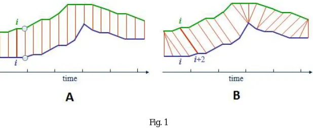
Consider a situation in which a HCI interface is subject to dynamic interaction with a vast variety of individuals belonging to different geographical zones. In such case, it is highly unlikely that the interface will receive human voice which is similar to the voice in which the interface itself was trained. For example: say the interface was trained in American accent of the English language, the interface will make serious mistakes while interacting with a Chinese person, since the Chinese person talks in English very much differently than a native American. Moreover, it may also happen that the interface might make serious errors while talking to an American itself, since the speed of elocution for which the interface was trained might be too slow or too fast in comparison to the speed in which the user interacting might talk, thereby creating several errors.
To elaborate these challenges in speech recognition, consider the following mathematical treatment. Consider
{ 1, 2, … … , } – which is the pattern to be tested, where is a vector representation of frame of speech at time and is the total number of such frames.
The above sequence is to be tested with a set of preset sequences stored in the system { 1, 2, … . , } where each sequence can be similarly represented as above as a set of vectors representing speech input at a particular unit time. The objective of any pattern recognition technique to be used to compare these two sequences for equivalence is to find a similarity between T and any one sequence from the set{ 1, 2, … . , }. Any such pattern recognition technique must address the following issues that may arise [1]:
1. As in our previous example, the rate at which different people talk is different, and hence T and S vary on the time axis and may be of different durations.
2. The length at which different syllables are pronounced varies significantly and hence the sequences T and S
may not at all fit in any simple well prescribed manner.
3. Though there might be local similarity in patterns, they might differ globally; hence the technique must represent speech as composition of spectral vectors and must provide for both local as well as global dissimilarity measures.
DTW provides a solution to such pattern recognition challenges by comparing two sequences irrespective of their time alignment, by distorting the time axis.DTW attempts to compare two patterns of speech irrespective of their variations on the time axis. This can be better understood from the figure given below [2].
Fig. 1
B. Mathematical Treatment:
Consider two sequences- { 1, 2, … . . } and { 1, 2, … . . }where the former is the input sequence and the latter
is the preset sequence stored within the interface.These sequences can be arranged to form a grid where each point
( , ) will correspond to the extent of dissimilarity between the elements and . The extent of dissimilarity is the distance measure (the metric for distance measurement can be suitably chosen).The alignment of two sequences can be geometrically shown as follows [3]:
Fig. 2
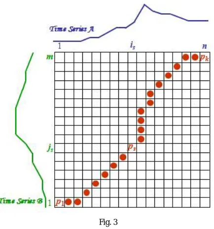
A warping path comprised of frames{ 1, 2, … . . , } will then map the frames of the sequences to one another, such that the distance of the overall path is minimized.
Following example elaborates the characteristics of the warping path:
Fig. 3
( , ) = ∆ ( )
Where ∆ ( )the warping function and p is is the number of points to be traversed.
C. Interpretations from DTW:
Following can be interpreted according to the theoretical postulation provided above:
1. The line = (the diagonal) in Fig 2 represents a perfect alignment of two sequences with each respect to one another.
2. If the warping path, which has the minimum accumulated distance (cost), is in close proximity with the diagonal, then the two patterns can be considered similar.
3. The extent of deflection of the warping path from the diagonal shows the extent of dissimilarity between the
two sequences with respect to time.
4. The DTW algorithm is a recursive algorithm as it uses dynamic programming. It will traverse many paths across the grid, calculate the costs of each path, select the path with minimum cost and then retrace the path to the starting point. Hence, the implementation of the algorithm must facilitate to remember the nodes which are traversed, to retrace the path in the future.
5. Since there can be many paths which must be traversed to find the optimal path, the algorithm must restrict
itself to paths which obey certain criterions which will optimize the process of executing DTW.
D. Constraints on DTW for Optimum Processing Time
Following are the constraints that need to be adhered to in order to implement the DTW algorithm efficiently. Any paths traversed, which violate any of these constraints must not be taken into consideration while choosing the optimum path.
1. Monotonicity: This condition ensures that subsequent frames must always be compared with frames ahead in
time. The algorithm must not go back in time to find similarities.
2. Continuity: This ensures that the warping path is continuous, and that the algorithm does not miss out any important feature in the sequences.
3. Boundary Condition: The algorithm shall consider only the paths which start and end at the opposite vertices
of the grid.
4. Warping Window: The warping window ensures that the algorithm considers the paths which lie within a certain proximity of the diagonal; the algorithm rejects the paths which deviate extensively from the diagonal. 5. Slope Constraint: This constraint dictates that the warping path shall not be too steep or too shallow. It avoids
the matching of very short sequences to very long ones and vice versa.
E. Advantages
1. It is very easy to train the interface with DTW since the end user controls it (unlike other techniques like neural networks in which user control is compromised to a certain extent).
2. DTW is independent of the language of speech as long as the patterns match with each other.
3. DTW provides intuitive distance measurements in samples.
F. Disadvantages
1. Since many paths need to be traversed, the DTW technique has an inefficient time complexity (around O(N2)). 2. DTW cannot be practically implemented for a large set of reference sequences.
III. HIDDENMARKOVMODELS(HMM)
A. Introduction
Automatic continuous speech recognition (CSR) has many potential applications which includescommand and control, transcription of recorded speech, dictation, searching audio documents and interactive spoken dialogues. The speech recognition systems consists of a set of statistical models that represent the various sounds of the language to be recognised. Since speech can be encoded as a sequence of spectral vectors spanning over an audio frequency range and has temporal structure, the hidden Markov model (HMM) provides a framework for developing such models.
The modern HMM-based continuous speech recognition technology were found in the 1970’s by groups at Carnegie-Mellon and IBM. They introduced the use of discrete density HMMs and then later at Bell Labs, continuous density HMMs were introduced[4].
B. States in HMM
Fig. 4
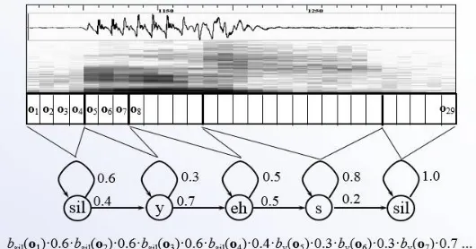
Consider the example shown in figure 4, which elaborates the concept behind HMM: The word ‘CAT’ is divided into three phonemes, ‘k’, ‘ae’, ‘t’. The time span of utterance of the phonemes is indicated on the transition arrows.For each HMM, the probability of the best state sequence in the observed speech is determined. Then the HMM which best matches (probability) the observed speech is selected.The state sequence of this selected HMM determines the required word sequence [5].
C. Architecture for HMM
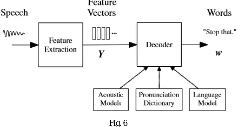
The audio waveform from a microphone is first converted into a sequence of fixed size acoustic vectors Y1:T =y1,...,yT. This process is termed as feature extraction.
The decoder attempts to find a sequence of words w1:L=w1,...,wL which is most likely to have generated the sequence Y, i.e. the decoder tries to find
w= arg max{P(w|Y)} eq (2.1)
However, asmodelling P (w|Y) directly is difficult,Bayes’ Rule is applied to transform equation (2.1) into the equivalent problem of finding:
w= arg max{p(Y|w)P(w)} eq (2.2)
The probability p(Y|w) is determined by an acoustic model while the prior P(w) is determined by a language model.
Fig. 6
The basic unit of sound which is represented in the acoustic model is the phone. For example, consider the word “bat”. It is composed of three phones /b/ /ae/ /t/. For English about40 such phones are required.
For any given w, phone models are concatenated to make words as defined in the pronunciation dictionary. Thus the corresponding acoustic model is generated. The parameters of the phone models are projected from training data which consist of speech waveforms and their orthographic transcriptions. The language model typically is an N-gram model. The probability of each word in this model, is conditioned on its N−1 predecessors. The N-gram parameters are estimated by counting N-tuples in appropriate text corpora. The decoder then searches all possible word sequences using pruning to remove unlikely hypotheses.Thus it makes the search tractable. At the end of the utterance, the most likely sequence of words is obtained.
The interface needs to be trained to adjust model parameter for better probability of recognition. Audio data from many different sources are used as input to the prototype HMM. The HMM will adjust the model parameter accordingly. Once the training is complete, unknown data can befed for recognition[4].
D. Advantages
1. It is very rich in mathematical structure as Bayes Rule is used to find the most probable sequence of words. 2. HMM’s can be trained automatically and are simple and computationally feasible to use.
E. Disadvantages
IV. ARTIFICIALNEURALNETWORKS(ANN)
A. Introduction
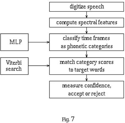
There are four basic steps to performing speech recognition by the use of Artificial Neural Networks (ANN). These steps are elaborated in the diagram below.
Fig. 7
We first digitize the speech that we want to recognize. For telephone speech sampling rate of 8000 samples per second is used. Then, we compute the features which represent the spectral-domain content in this speech (regions of strong energy at specific frequencies). These features are computed at an interval of10 msec.This one 10-msec section is called a frame. A neural network is then used at each frame to classify these features into phonetic-based categories. The final step includes a Viterbi search in which the neural-network output scores are matched with the target words (the words that are assumed to be in the input speech).Thus the word that was most likely uttered is determined.
The results can also beanalysed by observing the confidence in the top-scoring word. If the confidence falls below a pre-determined threshold,the word is rejected as out-of-vocabulary [8].
B. Architecture and Mathematical Treatment
The input digitized waveform is first converted into a spectral-domain representation. Depending on the recognizer used,one of the two sets of features may be used. For the general-purpose recognizer, twelve mel-frequency cepstral coefficients (MFCC coefficients), twelve MFCC delta features indicating the degree of spectral change, one energy feature, and one delta-energy feature (for a total of 26 features per frame) is used. Cepstral-mean-subtraction (CMS) of the MFCC coefficients is calculated to reduce the effects of noise. For the latest digit recognizer, twelve MFCC features with CMS, one energy feature from MFCC analysis, twelve perceptual-linear prediction (PLP) features with noise reduction by RASTA processing, and one energy feature from PLP analysis (for a total of 26 features per frame) can be used.
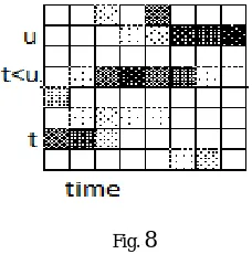
The features in the context window are sent to a neural network for classification (26 features per frame in 5 frames = 130 features). The neural network results in a classification of each input frame, measured in terms of the probabilities of phoneme-based categories. Context windows for all frames are sent to the neural network, and from the result obtained, the probabilities of phoneme-based categories is mapped over time in a matrix as shown in figure 8. In this figure, the word ‘two’ is to be recognized.The shaded regions in the t, t<u, and u categories indicate the greater probabilities at the indicated times.
Fig. 8
The target-word pronunciations are expanded into a string of phonetic-based categories. The best path through the matrix of probabilities is found using Viterbi search for each legal string. The recognition output is the word string obtainedfrom this best path [6].
Fig. 9
After obtaining the matrix of the variation in phonetic probabilities over time, we search for the word that best fits the matrix. For that, we first need to compute a set of legal strings of phonetic categories. This set of legal strings depends on the words that we want to recognize and the possible order of words. Thus we combine the pronunciation models for each of our words with a grammar. In the example shown in figure 9, we have a simple search path that can recognize only "yes" or "no". Both the words must be preceded and succeeded by silence. While searching, we transition from one state to a new state if the probability of the new state is greater. At the end of the search, we obtain the score for the most likely category sequence and the path that was used to generate the best score. We can easily determine the corresponding word (or word sequence) from this obtained path. This word has the best match to the input data, and it is therefore the word that was most likely uttered.
C. Advantages
2. Neural networks can be very powerful speech signal classifiers. A small set of words could be recognized with some very simplified models.
3. No strong assumptions about the statistical distribution of the acoustic space: this is a theoretical property of ANN, unlike standard HMM which assumes that all the subsequent input frames are independent, that in speech is clearly not realistic.
4. Parsimonious use of parameters: the use of a distributed model like ANN allows good results to be obtained
with a reduced number of parameters[7].
D. Disadvantages
1. The efficiency of the interface depends largely on the range of Mel Frequency Ceptstrum Coefficients.
2. The number of hidden layer neurons depends on the number of words to be recognized. Larger the number of
words, more the training time of the interface.
V. CONCLUSION&FUTUREWORK
This paper discusses the three popular techniques used for Speech Recognition in the areas of Human Computer interaction viz. Distance Time Warping, Hidden Markov Models and Artificial Neural Networks. We would like to conclude by enlisting the following decisive insights on the applicability of these techniques to various types of interfaces having disparate requirements:
1. Distance Time Warping (DTW) is the best suited efficient method in case of interfaces that are to be trained for a single speaker (human voice or even machine generated voice), use limited vocabulary, and for use in trivial applications that do not aim scalability.
2. Hidden Markov Model (HMM) suits best when interfaces require frequent manipulation in the parameters for
speech recognition. HMM is a probability based statistical model, and hence is highly flexible for such parametric changes and thereby supports multiple speakers and a large vocabulary of words. It is also easy to implement HMM once the algorithm and parameters are decided.
3. Artificial Neural Networks (ANN) finds felicitous applications in systems that aim for high scalability and ubiquity and in those which demand continuous speech recognition. ANN are best to use in such systems for two peculiar reasons: firstly, because they facilitate the use of many parallel processors thereby providing the tremendous computing power required for continuous speech recognition; secondly, because ANN can foster the development of new undiscovered internal training techniques which might eventually perform better than the earlier ones.
REFERENCES
1. Rabiner, Juang, Yegnarayana , “Fundamentals of Speech Recognition”, Pearson Publications
2. Jo Criel1 and Elena Tsiporkova, “Gene Time Expression Warper: a tool for alignment, template matching and visualization of gene expression time series”,www.psb.ugent.be/cbd/papers/gentxwarper/DTWAlgorithm.ppt
3. Donald J. Bemdt and James Cliffor, “Using Dynamic Time Warping to Find Patterns in Time Series”, AAAI Technical Report, pg 359-368, 1994
4. Mark Gales and Steve Young, “The Application of Hidden Markov Modelsin Speech Recognition”, Foundations and TrendsinSignal Processing, Vol. 1, No. 3 (2007)
5. LAWRENCER. RABINER, “A TutorialonHidden Markov Models and Selected Applications in Speech Recognition”, IEEE Log Number 8825949, VOL. 77, NO. 2, 1989
6. Rabiner and Juang. Fundamentals of Speech Recognition. Chapter 6.
7. Wouter Gevaert, Georgi Tsenov and Valeri Mladenov, “Neural Networks used for Speech Recognition”, Journal of Automatic Control Vol 20, pg 1-7, 2010.