Floating point roundoff error analysis of the adaptive exponential sliding window RLS algorithm for time-varying systems in the presence of noise

Floating Point Roundoff Error Analysis of the Adaptive Exponential Sliding Window RLS Algorithm

for Time-Varying Systems in the Presence of Noise

by

S .H. Ardalan

Center for Communications and Signal Processing Department of Electrical Computer Engineering

North Carolina State University

February 1986

Table of Contents

Page

1.1 Introduction 1

1.2 The RLS Algorithm 2

2.1 Brief Summary of Results 2

2.2 Paper Organization 3

3.

Recursive Least Squares Algorithm: Infinite Precision 4

4. Floating point Roundoff Error Models 5

5. Floating Point Implementation of theRLS Algorithm 6

5.1 Desired Signal Prediction 6

5.2 Prediction Error Calculation 7

5.3

Weight Vector Update Recursion

7

5.4 Weight Error Vector Norm and Mean Square Prediction Error 10

6. Summary of Results 11

Prewindowed Growing Memory Algorithm ('A=1) 11

Exponentially Windowed RLS Algorithm ('A

<

1) 12

7. Termination of Updating for Stationary Systems 15

8. Derivation of Floating Point Roundoff Effects on theRLS Algorithm 17

Prewindowed Growing Memory RLS Algorithm ('A=1) 20

Exponentially Windowed RLS Algorithm ('A

<

1)

22

9. Extension to the Least Mean Squares Algorithm 25

10 Simulation Results 28

11. Summary 30

12. Appendix A 31

13. AppendixB 32

14. References 35

Floating Point Roundoff Error Analysis

of the Adaptive Exponential Sliding Window RLS Algorithm for Time-Varying Systems in the Presenceof Noise

by

S. H.

Ardalan

Abstract

1.1 Introduction

The Recursive Least Squares (RLS) algorithm has found wide application in adaptive filtering problems [1.2,3]. In particular, the algorithm offers very fast convergence and tracking capability. Unlike the L~fS algorithm, the convergence of the RLS algorithms is independent of the signal statistics, i. e., eigenvalue spread of the signal covariance matrix. This has lead to the applieation of the RLS algorithm to many adaptive filtering problems. However. finite wordlength effects on the digital implementation of this algorithm have not been thoroughly analyzed until recently. In

[4]

the error pro-pagation of the prewindowed growing memory ( A= 1) and the the exponential sliding window ( 'J\.

<

1 ) RLS algorithm for time varying systems was analyzed. In the paper. the propagation of a single error in the continuous use of the various algorithms was studied. It was shown that the effects of a single error decays exponentially for the conventional RLS algorithm, where the base of the decay is equal to the forgetting factor A. As pointed out in

[4],

however, little work has appeared in the literature concerning finite word length effects on the performance of adaptive RLS algorithms. In particular, finite precision arithmetic produces perturbations on the estimation of the system impulse response at each iteration. Furthermore, it is of interest to analyze the effects of each operation on the performance of various algori thrns. As will be shown in this paper. cer-tain finite precision errors tend to destabilize the algorithm while some only cause ~l bias in the estimates. On the other hand, some operations do not effect steady state perfor-mance at all. For these reasons, the analysis of the effects of all errors introduced at each iteration is of interest.

Recently a fixed point and floating point error analysis of the Least Mean Squares (L:vfS) algorithm was presented in

[7].

In [8] a fixed point roundoff error analysis of the prewindowed growing memory RLS algorithm was presented. In that paper. a closed form solution to the excess mean square error due to fixed point arithmetic is derived. It

\vas found that the mean square prediction error diverged linearly with the number of iterations prior to the freezing of adaptation (due to the Kalman gain vector approaching zero ).

2.

1.2

The RLS Algorithm

The RLS algorithm can be summarized as follows: The desired signal d( n) is predicted from the input samples by convolving the input samples with a weight vector. The prediction error is then calculated as the difference between this signal and a measure-ment of the desired signal which may be corrupted by noise. The prediction error is used to update the weight vector to minimize the accumulated sum of the square of the resi-dual error. The weight vector that minimizes this criterion at each iteration is written recursively. This leads to the Kalman gain vector which when multiplied by the scalar prediction error forms the weight vector update. Therefore, for the purposes of this paper, the algorithm involves two primary calculations. The calculation of the prediction of the desired signal d(n) through an inner product of the weight vector and the vector of delayed elements of the input samples; and the calculation of the weight vector update. The weight vector update involves the calculation of the weight vector correc-tion through the multiplication of the Kalman gain vector and the scalar prediction error and adding the correction term to the current estimate of the weight vector.

For the purposes of analysis we assume that the Kalman gain is calculated with infinite precision and a floating point quantized version is available. This assumption is based on the fact that the Kalman gain can be calculated using different algorithms and that as a preliminary step we are attempting to isolate the causes of error in the floating point implementation of the algorithm.

•As in the case with the floating point error analysis of fixed digital filters [9,10J and the L~IS algorithm in [7] the errors introduced by floating point operations are modeled as follows: For summation fl(x+y)=(x+y)(l+e) and for multiplication ti(xy)=xy(l+&). The relative error terms e and S are zero mean white independent random numbers. They are uncorrelated with x--y and xy. Using the above models the errors introduced by floating point implementation are incorporated into the algorithm.

2.1 Brief Summary of Results.

of the forgetting factor, J\. ln order to reduce the effects of additive noise and the floating

point noise due to the inner product calculation of the desired signal, ,\ must be chosen

close to one. On the other hand, the floating point noise due to floating point addition in the weight vector update recursion increases as A-i. Floating point errors in the calcula-tion of the weight vector correccalcula-tion term, however, do not affect the steady state error and have a transient effect. For the prewindowed growing memory RLS algorithm, exponential divergence may occur due to errors in the floating point addition in the

weight vector update recursion. However, if Ais decreased the errors due to floating point operations in the weight vector update addition decay exponentially and a more stable algorithm results. This is in agreement with

[4].

However, additive noise and floating point noise in the calculation of the desired signal will produce a bias in the estimate of the optimal weight vector for A

<

1. Moreover, if 'A is close to one but not equal to one we predict that divergence may occur.

The results for the L~[S algorithm show that the excess mean error due to floating point

arithmetic increases inversely to loop gain for errors introduced by the summation in the

weight vector recursion. The calculation of the desired signal prediction and prediction

error lead to an additive noise term as in the RLS algorithm. Significantly, as in the RLS

algorithm, the precision used in the ralcu lat ion of the weight vector correction term does not effect steady state performance.

2.2 Paper Organization.

The paper is organized as follows: In the next section the infinite precision RLS algorithm is presented, followed by a review of floating point error models. In section 3, the floating point errors are incorporated into the RLS algorithm. It is shown that the mean square prediction error is related to the mean value of the weight error vector norm which is equal to the trace of the covariance matrix of the weight error vector. In section 6, a sum-mary of the expressions for the weight error covariance matrix is presented. In section';',

4

3. Recursive Least Squares (RLS) Algorithm: Infinite Precision

The Recursive Least Squares (RLS) algorithm is used to solve the system identification

problem as shown in Figure 1. In the figure x(n) is the input sample to the system and z(n) represents the output of the system corrupted by additive noise v(n). The system is

described by its impulse response Wit. i=O, ...,i\r-l which is convolved with the input to

pro-duce the output signal d(n) as follows:

N-l

!- • ~T

d(n)

=

2:

wix(n-l)=w

xfn)

i=O

The measured output is corrupted by additive noise v(n),

z(n)

=

d(n)

+

v(n)

(3.1)

Here we assume that the impulse response wf: has insignificant terms beyond ~ samples. The notation x(n) signifies the vector of the last N samples while w!-is a vector represent-ing the ~ values of the impulse response:

x(n)=[x(n), x(n-l), ... x(n-~+l)]T

(3.2)

The RLS algorithm produces the weight vector w(n) which is an estimate at time n of the

~ ,

true impulse response w . The RLS algorithm operates on x(n) and z(n) to obtain an esti-mate ofwi: based on the previous estimate as follows:

where

is the prediction error and

w(n)

=

w(n-1)

+

K(n)

e(n)

e(n) = z(n) - d(n)

d(n)=w

T(n-l)~(n)

(:3.3 )

(:3. -t )

is the prediction of d(n) based on N previous samples of ~(n). The Kalman gain can be

shown

[1]

to be

(:3.6 )

5

to the weight vector w (n) and writing w(n) recursively. For the p rew in do wed growing

memory RLS algorithm A =1. However for time varying systems in which the impulse

-tc

response \v may change, A

<

1is chosen. In this case the algorithm is referred to as the exponential sliding window RLS algorithm. For A

<

1old samples lose their significance

in the calculation of

w(

n).

It has been

shown that in the infinite precision

RLS

algorithm

w(n)

converges to wr: when the additive noise source v( n) is a white random process and ,\=1.

The issue addressed in this paper concerns this convergence of w(n) toward wI- when the

RLS

algorithm described in equations (3.3-3.5) do not have infinite precision arithmetic but are performed on real machines using floating point arithmetic.

In order to evaluate this convergence, we define

(:3.7) where the primes denote quantities determined using floating point arithmetic. Thus, ft'(n) is the weight error vector denoting the difference between the floating point estimate

, I:

W (n) and the true impulse response w

In what follows we show that

ft

(n) can be expressed as the sum of two terms:

tl.'(n) =

x-fn)

+

!ll(n)

(3.8)

Here, ili.(n) in the absence of additive noise is the excess floating point error vector which would not exist if infinite precision arithmetic could be used. In the absence of floating

point errors, x.(n) would be the only component of the weight error vector and it has been

shown

[11

that x,(n) would approach Q as n gets larger. However, floating point arithmetic also produces errors in ;dn) so that it does not approach Q as n increases. Thus both x(n) and !ll(n ) contribute to the estimation error.

In the next section we describe the floating point round off error models and include them

in the floating point RLS algorithm.

4. Floating Point Roundoff Error Models

In this paper the errors introduced by floating point operations are modeled as follows: For multiplication

(-t.l)

6

of

x.y

and

(x·y).

It has been found [0.8] that

i<~=E(€:!)-(O.18)2-:!B

where B IS the

number of bits used to represent the mantissa.

For addition

fl[x+y]

=

(x+y) [1+?>] (4.2)

where 0 is the relative error modeled as a zero mean random variable with variance

a:.

The actual distribution of 8 and e are not important in what follows as long as the

h

assumption that each error term is a zero mean, independent in time, random variables is

valid.

Note that in floating point operations, addition and multiplication both introduce errors.

whereas, in fixed point operations (assuming no overflow) only multiplication introduces error.

5. Floating Point Implementation of the RLS Algorithm

In

this section we incorporate the errors introduced by the floating point implementa-tion of the RLS algorithm into the algorithm.

5.1 Desired Signal Prediction

Consider the calculation of the prediction of the desired signal through the inner

pro-duct (3.5). Let p(n) denote the error introduced by floating point operations in the calcu-lation of the inner product. Then,

(.S.l )

For the above equation d' (n) is the prediction of the desired signal using the floating

point RLS algorithm and w'(n) is the floating point weight vector. The primes denote

the floating point variables as opposed to the infinite precision variables of (3.1-:3.6). Denoting the floating poir:t errors produced in the summation and multiplication

7

(5.2)

[xo(n)w'o(n)+x1(n)\v' t(n)Jut(n)

+ ...+

[XO(n)w' O(n)

+...

+

x~_l(n)w'

:'r-l(n)}U:'I-l(n)

'vVe assume that

E1(n)

and

ui(n),

i=O, ... ,N-l are zero

mean

white random sequences and therefore p (n) is a zero mean white random sequence. vVe have

[-tL

N-l

a

_l;

=

E[pz(n)]

=

(fez

I

a;

E[w'~(n)l

+

(5.3)

k=O

'1

The expression ((5.3) for (To. can be written in terms of the autocorrelation matrix R

p x

and the optimal [Wiener) vector w :c as in

[4].

But this assumes that ~ '(n) converges.

\Ve

will show, however, that w '(n) might diverge and thus (J'2 will diverge also due to

- p

floating point errors introduced in the weight vector update recursion. Nevertheless. the point to consider is that prior to divergence

(f~

depends on the floating point noise sources and thestatistics of x(n) and w '(n).

5.2 Prediction Error Calculation

Next consider the floating point error introduced In the computation of the prediction

error (3.4). We have.

...

e{n )

=

[z(n) - d'(n)](l+&(n)] .

(.).-!)

where we assume that the relative error

&(?-)

is a zero mean white random sequence. If we substitute (3.1) for ztn) and

(.5.1)

for d '(n) then we can write

where we have neglected t.he ~~(~ond order noise term (J(n)&(n).

5,,3 Weight Vector t·pdate Recursion

equation (;3.;3) . .Assuming that the Hoaring point quantized Kalman gain vector elements are available at each step, the recursive update equation for each weight vector element

including floating point noise sources is

w.'(n)

=

{w.'(n-l)

+

K.(n)e'(n)[l+J.L.(n)]}[l+Ci.(n)]

1 1 1 1 1

(.5.6)

where J..L.(n) and a.{n) are the floating point noise sources due to multiplication and

addi-1 1

tion respectively. Expanding (5.6) and neglecting second order noise terms we obtain,

If we define the diagonal matrices,

q"rN(n )=diag(Ci.(n)+J..L.(n)1

..~ 1 1

then the weight vector update equation becomes

w'(n)

=

w

'{n-L)

+

!S(n)e'(n)

+

Ct:'[N(n)w'(n-l)

+

<t>:-;N(n)~(n)e'(n)

Substituting for e{n ) from (,5.6) and neglecting second order noise terms we obtain.

~'(n)

=

~'(n-l)

- !S(n)x

T(n)[~'(n-l)

-

w"'] -

K(n)l1(n)

-where we have defined.

11 (n) == v(n) - ~(n) .

(,5.9)

(5.10)

(5.11)

(3.7). Therefore. subtractinc \v<

.~

obtain.

9

from both sidps of (.).1:2) and substituting

(:3,;.. )

we

ft'(n)

=

ft'(n-i) - K(n)x T(n)H'(n-i) - 8(n)K(n)x T(n)ft'(n-i)

+

<i>NN(n)K(n)

X

T(n)ft'(n-i)

+

cxNN(n) [ft'(n-1)

+

w

"'1-

K(n)TJ(n)

(5.13)

Collecting terms,

ft'(n)

=

[I -

K(n)x T (n) -

~N(n)

K(n)x T(n)

+

_{u NN(n)]ft'(n-1)}

+

u

N0I(n)w'"

- TJ(n)!S(n)

(5.14)

where

(.1.16)

Define the matrix

(.5.17) and the vector

(.5.18)

Then substituting into (.5.15) we get

(.S. 1~))

Equation (5.19) represents the recursive update equation of the weight error vector in terms of the noise sources due to floating point operations. For infinite precision. and if

v(n) = 0,

10

which is the exact recursion for the infinite prectsron update equation of the weight error vector.

5.3 Weight Error Vector Norm and Mean Square Prediction Error

We can express the floating point prediction error (5.5) using (3.7) and (5.12) as,

e'(n)

=

(-xT(n)ft'(n)+T\(n) )[1 + 8(n)]

Define the Mean Square Prediction Error:

IT

;(n)

=

E{e'2(n)}

=

E{xT(n)ft'(n)ft'T(n)x(n)}[l

+

ail

+

a~

Or,

where,

a, =

E{x(n)~

T(n)}

and,

Noting that,

and

we can write (5.23) as follows,

cr;(n)

=

cr;E{lla'(n)112}(1 +

crl) +

cr~

(5.21)

( - ')'))

~0._-(5.23)

(5.24)

(5.25)

(5.26)

(

U._4

-

.)-)

(5.28)

From (5.28) it is clear that the mean square prediction error is related to' the expected value of the norm of the weight error vector .t!'(n). From (5.26) the expected value of this norm is related to the covariance matrix of the weight error vector. In the next section \ve

l1

6. Summary of Results

As was pointed out in section :3, the Heating point weight error vector can be expressed as the sum of two vectors.

ft'(n)

= x.(n)

+

!It(n)

The covariance of the weight error vector is thus,

(6.1)

(6.2)

where we have neglected the cross correlation between x.(n) and ill.(n) (see section 8).

In the following paragraphs we present expressions for Rx(n) and Ru,(n) for the stationary and time varying RLS algorithms. Using equations (5.26) and (.5.28) the mean square prediction error and the expected value of the weight error vector norm can be computed by substituting for Rij .

[n the expressions to follow.

is the variance of the floating point noise due to addition III the weight vector update

recursion

(5.6).

The variance.

is the sum of the variance of the additive noise v( n) and the noise due to the vector inner product calculation of

df

n )(5.1). In the derivation leading to the results, the input sam-ple x(n) is assumed to be a zero mean, independent in time. white Gaussian random

vari-''l

able with variance

fT;.

r

1 . q 1

't-

4 diag

[Wi

-j

+ -.-)

(T('( a~

12

(6.3)

1

Rx(n)

=

ft(O)ftT(O)~

e; . e-2-Yr eQ

fT,~

n- (6.4)

..Assuming updating does not stop, an examination of (6.3-6.4) shows that the RLS algo-rithm diverges as the number of iterations (n) becomes large. This divergence is exponential with respect to n. It is observed that the divergence terms are due to floating point errors in the calculations of the weight vector update

(3.3),

i.e .. a.(n). Also, the

1

steady state solution is independent of the floating point error introduced in the calculation

of the weight vector correction term . i.e .. f.1i( n). Hence, no steady state degradation

results if low precision is used in the calculation of these terms, i.e., K(n)e'(n) in (3.3). If updating stops after nT iterations then the following expression holds for R,I,(n) pro-vided n is large but small compared to

~

such that eQ 'T,; :::::1.

(J~

(6.

.5)

Assuming no errors in the calculation of the update for w(n), and (T2 - 0 it is shown in

- a

section 8 that

'l

lim Rij(n)

=

ft(O)ft

T(n ) l;;- e -2-Y r

+

1-

0": I

(r,~ --0 n" n

a;

where"t«

=

0.57721 is Eulers constant.

(6.6)

In other words, the errors due to the additive noise and inner product calculation of the

prediction of the desired signal are averaged out by the algorithm. They will not cause a bias in ~ [n ) as it converges to ~ ". However, they will contribute a noise term with

variance 0"11'! to the prediction error as shown in 15.28). Notice that the steady state RLS solution is independent of the initial condition. However, with Hoatin~' point errors the

stea.iv state result depends on the initial condition.

13

[n the case of the exponential sliding window RLS algorithm the following results are obtained:

where,

and

u = a~

-

2(1-A)

(6.9)

(6.10)

The matrix C·(~[) collects the terms for which i

<

M, where the index :Vf is defined as the index for which A

~1

«

1 .or

~1

>

1

i-A

..An examination of the results reveals a tradeoff in the choice of the forgetting factor A. In

order to reduce the contribution of the additive noise and vector inner product floating point noise in the calculation of ci'(n) to the estimation of w~, we must choose Aclose to one. On the other hand in order to track a time varying system Amust be smaller than

one. Furthermore, as 'A. becomes close to one, U in (6.9) may become positive. This in

turn leads to exponential divergence or an amplification of the estimation error due to the floating point addition in the weight error vector update as predicted in (6.6) and (6.7).

[f we choose A such that u<O~ then the steady state weight error vector covariance matrix

becomes.

(6.11)

If (1~

«

2(1 - A) then (6.11) becomes,

L4

The above expression clearly shows that increasing 1\ ( A-I ), in order to reduce the

mean square error due to additive noise amplifies the Heating point error due to the addi-tion in the weight vector update recursion (

(T(;).

Decreasing X. for tracking time varying systems improves stability ( in the case of the can ventional RLS algorithm) and reduces the floating point error due to this operation but causes an increase in the bias due to

additive noise.

In the next section conditions are derived for 'the early termination of weight vector

updating in the floating point RLS algorithm for stationary systems. The conditions

15

7. Termination of Updating for Stationary Systems

..An examination of the weight vector update recursion (3.3) reveals that the condition for

the ith component of the weight vector not to be updated is,

(7.1)

(- oJ)

1 . _

where B(l is the number of bits used to represent the mantissa of the weights. This expression is similar to the condition presented in

[7)

for the floating point LNIS

algo-rithm. Since (see Appendix ..-\'),

E{IIK(n)112}~

[

1 - A

]2

N"

1-Ak a :_x

then,

(7.3)

Termination of updating results after the weights approach the true weights ( wi(n)::::wi' ) and the major component of the prediction error is the noise source ll(n) consisting of additive noise and floating point roundoff error noise. Hence. (Te:!~::(J~. Therefore, the

condition (7.1) leads to,

:! -')B

[

1 - A

1

2 2

~

"

Iw·T!

k (jTl< ~ 1

1 - A "1:

For A=l updating terminates after nT iterations where.

For A

<

1, nT is,

o-J(1 - ~' ( j

"'"' J ., ]

In(l

-2

-8"1

Wi' (min)

I

lnx

~ote that updating never terminates

if

- 8 -1

1 "(·)1

2 ' f wi .min

A<l-(7.4)

(7.5)

16

From the (7 .

.5),

the prewiridowed growing memory RI.JS algorithm will terminate updating

when the additive noise vtn ) is very small. In fact, it is possible that the algorithm will terminate after the first )i iterations if a;~O. In this case"

(7.8)

If rr~ is large and B_u is also large, then nT can be large enough such that the steady state

1r

results of this paper are valid. Furthermore, in many practical cases Wi :::: 0" for some L

in which case updating may never terminate for the ith component of the weight vector. In cases where nT is small compared to

~,

equation (6.5) must be used for the steady

(J' (;

17

8. Derivation of Floating Point Roundoff Effects on the RLS Algorithm

If

we write the recursion (5.19) for

ft

'(n) in terms of the initial condition t! '(0), then we obtain

ft'(n)

=

tDl

[1-K(i)x

T(i)

+

r3NN(i)]

]t!(0)

+

i~l

(j

~l

[I -

K(j)x

T(j) +

r3NNU)] ]f.(i)

~ote that we define

Define the weight excess error vector as

(8.1 )

(8.2)

n

!1!(n)

=

2:

i=l (8.3)

.-\150 define

Then

ft'(n)

= x(n)

+

ili.(n)

(8.-t)

(8.5)

Neglecting the floating point noise sources in the matrix, ~~~(i),x(n) describes the con-vergence of the weight error vector towards ~. That is w (n) approaches

'ff

as n - x . In this case ~(n) represents an excess weight error vector due to floating point opera-tions in the algorithm. Since the elements of ~(i) are zero mean white random quantaties

~Ne can neglect the crosscorrelation between X (n) and ~ (nl. Thus. the covariance of

H'(n)

becomes,

18

'vVe now proceed to calculate

n n n

R'u(n)

=

E{Yl(

n)illT(n)}

=

E{

2:

2:

n

[1 - K(k)XT(k)

+

~NN(k)l

i=l j=i k=i+l

~(i)~T(j).

n-n

1

[I - x(n-m)KT(n-m)

+

~JN(n-m)l

m=O

(8.8)

A major simplification of (8.8) results when we note that

5...

(i)

and ~

(j)

are independent zero mean random vectors for i=t=j. Thus,

I==J

(8.9)

Hence terms where i=I=-j drop out in (8.8). Now,

where we have substituted (5.18) for

5...(i).

Before we proceed further. we make the assumption that x(n) is a white Gaussian sequence independent in time with

autocorrela-tion matrix.

The following relationships are established in Appendix .-\ where we have used the "averaging principle"

[5.6]:

E {K(k)KT(k) }

=:: [ 11

~~k

r:;

I

E {K(k)xT(k) }

=:: [ 11

~~k

l

I

E {K(k)X

T(k)X(,k)KT(k)}:::: [

I-A

]2

N

.»)

I l-X.k (.

+ ..

. '

Hence.

(8.11 )

(8.12)

(8.13)

R(~(i)_r: = IT~ diaz fV\,..'~l

19

Thus R~(i) is a diagonal matr ix. Since xf n ) is a white Gaussian sequence. when we take the expectation in (8.8) all terms involving the vector x(n) will yield diagonal matrices, Furthermore, in (8.8) all terms j:;=i drop out based on (8.9). Also, the elements of the matrix ~NN(n) are independent white random variables. Thus, the expectation operator will cause all off diagonal elements of (8.8) to become zero. Since diagonal matrices can be permuted, anticipating the expectation operator we can write (8.8) as follows,

where we have defined,

n 'l n

Rw(n)

==

L

ITi(i)

Il

=(k)

i==1 - k==i+1

(8.1.5)

Now, from (,).17) the elements of

f3

NN(k ) are zero mean. 'vVe have using

(.5.17),

(5.16),

(5.1 ),

(8.17)

Substituting (8.12), (8.13) and (8.18) into (8.16) we obtain

=(k)

=

[1 - 2(1-

A

1

+ [

1-A

]:!

(N+2)

+

<1',;

+

l-Ak l-Ak

In the above equations we have defined

, ' l 0) .,

(1;

=

IT~

+

(T~

+

(J'~

2

I

1-A 0)

[ 1_ Ak

1 (

N

+

2

)<1';

I (8.19)

(8.20)

Substituting (8.19) into

(8.17»

we obtain 0=0,1, ...

:'-1-1),

R'!I(n)=

±

fI

[1-

~(l-~) ~ 1T1~]

[<1',; diag[w/l

+IT~ [:=~i

j:!

1T1~II

i==1 k=i71 I-A

Using the approximation

[

. 1-1\

]2

<

<

1-Ak

e

<

<

1

20

(8.22)

we can write (8.21) as,

{

' [ ]

~

1 } (n-i) (T; -2(

1-'\)'~

1

( ) .l!, .~ [~

t)]

1-~ _ (j2I e k=-I ' "I 1-,\~(8.2;3)

Rwn

=.2..

(T~ diag Wj~ +

-i==l i-Ai

fJ;

II

The above result is valid for n large. The initial transient period is not accurately

predicted by" the above equation due to our approximations, in particular (8.22). The analysis to follow separately considers the two cases A

=

1for the prewiridowed growing

memory RLS algorithm and A

<

1 for the exponentially windowed RLS algorithms. The reason for this is that different steady state solutions and approximations apply for the two cases.

Prewindowed Growing Memory RLS Algorithm

(A= 1)

In this case (8.23) becomes,

In Appendix B we show that

_.J , . . 1 (n-i) (r,f -k=~-rI i

e e (8.24)

Q 1

~

k==i~l

Substituting into (8.~--t),

n 1

In -

_.

+-~)

I

-n+i+l

n(i+l) n

»

1

(,-) ,.'-\

\,~._.).!

21

n-i-~l

e n(i~l) ::::1

Now for (1~ small and n large,

Q. . . ,

~ -1 (r;

~e

i=l

From Appendix B,

· (l-e-n (T,~ )

= e- (1,; -'-_

1-e- (r,~

- (',; 1

:::::_e

-(8.27)

Hence

n

~ . 2 -i.r; _ q -6

~ 1 e -.;,.a_u

i=1

n

(T-e (

' )

n""

; aCt:;:: 0 , n

>

1 _(8.28)

(8.29)

If 0 I b 11 d 1 h a <T

~

n

3

n is arge ut sma compare to - ' J - sue that e . -==1, then (8.:28) reduces to

rr~ 3

and,

oJ

1

n ~~ 1 a~

- a2 diag[w.-]

+-

- I

j

3

U 1 n a~~ (8.30)

Assuming no errors in the calculation of the update for w(n), (J"2 - 0 and noting that

- a

(8.31 )

equation (8.26)reduces to,

Next consider the covariance of X (n) which contains the information regarding the con-vergence of the weight error vector. Define,

R..

(n)

=

E{ '( In)

~

T(n)}

'(

22

Rx(n)

=

ft(O)E

[/I[

[I-K(i)XT(i)+f):'iN(i)]

~~IO [l-x(n-m)KT(n-m)+f)~:'i(n-m)J

]H.T(Ol

(8.;34)

From (8.16)

n

Rx(n)

=

ft(O)

Il

=:

(i) ftT(O)

i==1

Substituting for

=:

(i)

from (8.19),

(8.35 )

where we have neglected terms of order O(i-2) . Now,

n i l

~_~

-

_.

==

In

n - -

_{o J ' C}

+

'V ;~~_\", = 0.57721

n

»

L

i=L 1 _n

Thus,

1

Rx(n)

=

ft(O)ftT(O)~

e-; · e-2-y •. ell,r;

n'"

Exponentially Windowed RLS Algorithm (A 1 )

Define

n

g(J\,n) =

2:

k=l

in Appendix B we show that

lim

g(A,n)==

n

+

_1_ I n -1

-x-t

1-1\ 1-A

Define

(8.37)

(8.38)

(8.39)

(8. -10)

From Appendix B.

n f(A.i,n)

=

,~

k=-=l-L 1

k

=

g(A,n) - g(A.i)

1-A

(8.-tl)

lim

f(A.~.n)~::(n-i)

- Ai -L _ l_ In _l_

Hence (8.23) becomes,

a

R ()_,~n

₌₌

~_~ {·}e(n-i) (T~·e-2(1-t\.Hn-i)eln(1-i\)A'+' i==l

R'lI(n)

=

~

{'}e(n-i)

cT,;

e- 2(1-A)(n-i)(1_A)2,\.'-1

i=l

Consider the index i=1\;I for which Ai

«

1 ,or M

>

_1_ then (j==O.1, ....N-1),

I-X.

(8.43)

n

Rt1J(n)

=

I

i=wI (8.-14)

where we have made the substitution

The matrix

CI(NI)

collects the terms for which i

<

~1.

~l-l ( . .

C(~[) ==

I

{'}e n-l)u(l_A)~~'''''

i=.l

(8.4.5 )

(8.46)

If 1)

<

0 as n becomes large

l')

e-u a- -v

'l

diag [Wi~~]

+

(1-A)2~ e _(8.-t8)

RdJ(n)

=

C(~I)

+

(T(;

e-u-l a- e -l'_l

x

If l,'>0 ,n large

-1

e(n - \{)u

e(n - M)v

diag ['Vi~2]

(1-I)

+

(1-A)2~ I

_(8.49)

R,I,(n)

=

C(Nf)

+

a" ₁

-v

u _{1 -u}

(T" -e

-e x

n

R\(n)

=

!itO)

n

=:(i)ftT(O)

i==1

where,

-()~

=(i)

=::

[1-2 (1-A)

+

(]~

1

I .::: e - I-i\i e

(1:

I-Ai

Hence

where we have used

~ 1 1 1

) --. ==

n

+

I n

-i~\ i-Ai I-A 1-'\

Thus,

where u is defined by (8.46).

(8.-t9)

(8.,50)

(8.,S1)

25

9. Extension to the Least Mean Squares Algorithm

In this section, the errors introduced by floating point operations in the L~IS algo-rithm are derived using the approach for the RLS algoalgo-rithm. In the L~lS algorithm the prediction of the desired signal and the prediction error are computed as in the RLS algo-rithm.

(3.3)

and (3.~). However, the weight update recursion is computed

by

replacing the Kalman gain (3.6) with the simpler expression

)'x(n),

\v(n)

=

\v(n-l)

+

t'x(n)e(n)

Forstability,

'Y

must satisfy

2

'Y

<

-A_max

\vnere A_max is the maximum eigenvalue of the autocorrelation matrix

(9.1 )

(9.:2)

Comparing (9.1) to (:3.3) we observe that the development leading to (8.8) in the case of the RLS algorithm can be carried out by replacing K(n) with ~x (n) for the L1;lS algo-rithm. Hence. for the LMS algoalgo-rithm. the floating point weight error vector becomes comes:

where

and

n

e

H'(n) =

n

[1 - 'Yx(i)xT(i)

+

~NN(i)l(O)

+

i=l "

(9.3)

(9.-t)

(9.5)

Note that the floating point errors, Q)n), 1..1)n), ()(n), ~(f1) now apply to the L~[S algo-rithm.

26

Note that :(k) isdiagonal. Hence, for the L~[S algorithm,

n n

R'll

=

L

Il

=(k)

E{f.(i)f.T(i)} i=l k=i-r 1

Or,

n .

R - ~ R n-l:::::: R (1 _

)-1

,II - ~ ~ v ~ V

i=l

(9.6)

(9.7)

(9.8)

(9.9)

(9.10)

[Note that v<l since

»<

<

\ve obtain.

1

'l for practical purposes). Substituting for R~ from (9.6)

cr-_x

Trace (R'll)

=

[fT(;

lI

w

o.: W

+

'"Y2(J"~;-;(J.;]

For ~ small. v - 1-2 "fa2_x from (9.8). Hence,

1

l-v (9.11)

(9.12)

Consider now the floating point errors introduced in x(n). From (8.15) \ve obtain for the L1;IS algorithm,

R'( (n )

=

ft (

0)ft T (0)Vn (9.1:3 )

Examining (9.13) we note that in the absence of floating point errors, lim va-0 IT1LlSt

a-A:

hold for the algorithm to converge. .Assuming -y to be small (this is the case in many applications of the L~lS algorithm) we can write (9.~) as

For stability

.} .J

v -... 1 - 2"\1(1'""

+ () ...

I X Ct

.)

2~a_x-

<

<

L

Hence,

Finally,

(9.1,))

(9.16)

(9.17)

The expected value of the floating point weight error vector is

E{ll.tt'(n)W} = Trace[Rx(n)

+

R,dn)] =

(J" (;II'v='c112

(9.18 )

From this expression it is clear that a tradeoff exists in the choice of the loop gain 'Y. In order to reduce the bias due to additive noise and the inner product calculation of the

desired signal prediction, ~ must be reduced. On the other hand, this amplifies the

float-ing point roundoff error due to the floatfloat-ing point weight vector update calculation. This

observation is similar to the tradeoff in the choice of the forgetting factor in the time

varying RLS algorithm. In both algorithms the precision used in the calculation of the

weight vector correction term has no effect on the steady state performance. This result

can be used to simplify the hardware realization of the algorithm.

In the absence of floating point errors and additive noise, O"~-o and

u(;-o.

Then (9.18)

reduces to,

(9.19 )

Thus the

L.:YlS

algorithm will converge to

the

true impulse response w' independent of the

initial conditions. The rate of convergence is proportional to the loop gain "y.

The expression for the mean square prediction error can be obtained from (.5.26) and

(5.:28) by substituting for E{

II.~d

n)

W},

where T¥,,·e have neglected the term

(jt~·

(f ..;!lw"ll~

28

10. Simulation Results

In this section the effects of floating point errors on the performance of the RLS and L~lS

algorithms will be presented through simulation. Using assembly level subroutines (frexp

and ldexp ) in U0iLX it is possible to quantize the mantissa of floating point numbers. In the simulations to follow the operations

(3.1)

through (3.3) for the RLS algorithm and

(3.1), (3.2) and (9.1) for the L~IS algorithm are carried out with various number of bits

allocated to the mantissa. In the simulations the taps of the weight vector are estimated from the input and output (desired signal) sequence of a white Gaussian noise process convolved with a 9 tap impulse response. In the simulations, the norm of the weight error vector.

where,

IS plotted in dB's against the number of iterations. The number of bits used for the

mantissa in the floating point operations are indicated by

Bet

for the floating point addi-tion in the weight vector update, B~ for the floating point calculation of the weight vector

update term ( K(n)e{n) ), and B" for the inner product calculation of the prediction of the desired signal. If the number of bits allocated to the mantissa equals 23, then this

corresponds to 32 bit floating point operations. In the Figures if B is not indicated for a particular operation then it is equal to 23 bits.

The effects of the forgetting factor, A, on the convergence of the RLS algorithm for vari-ous number of bits allocated to the mantissa in the floating point addition of the weight

vector update recursion ( Su ) is presented in Figures 2 and 3. All other operations are

carried out with 23 bit mantissas. In Fig. 2, B(X=9 bits, and the forgetting factor is changed. The variance of the additive noise (

cr; )

is 10-6 in both Figures. In the infinite precision case, the steady state weight error vector norm should decrease as the forgetting

factor approches 1 when additive noise is present. However. as Fig. :2 clearly shows, the

steady state error actually increases due to floating point errors (

Ctl(n) )

when A-l. which is in agreement with the theoretical result (6.12). In Fig. 3, we observe that the norm

decreases as the number of iterations increases for the infinite precision calculation when

.\=1. However, for 8_ct.=10 the steady state error increases with 1\.-1. For comparison. the finite precision and infinite prer ision ~f'Slllt3for ,\ -==O.!}9 are also presented.

Based on the theoretical results in sect ion 6. the number of bits used for B should not

tJ.

29

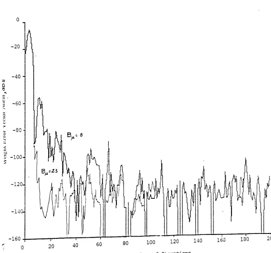
3 where B~ is changed from 2:) to 8 bits (

IT;

=

10--

6).

Very little difference is observed

bet,veen the two cases. According to the theoretical results of section 6, decreasing 1\

should increase the contribution of the floating point error, in the calculation of the

desired signal prediction, to the steady state weight error vector norm. This is verified in

Fig. 4 where B,,=9 bits and cr; =

o.

The steady state error decreases as A.-I.

Early termination of updating is examined in Fig. 5 for the prewindowed growing

memory case. Note that the steady state error increases approximately by 6 dB as Sex is decreased by one bit since, based on the arguments of section 7~ the steady state error is

proportional to a~ when the additive noise is verysmall (

a;

=

10-10 in this case).

In the Fast RLS algorithms [3,1] the Kalman gain exhibits large random changes,

although its norm should decrease as the number of iterations increases. This is

particu-larly true when a very small soft constraint is used. In these cases updating may never terminate and the divergence due to floating point errors predicted in this paper may well occur. This divergence phenomenon is examined in the simulations presented in Figures 6 and -;, where the Fast Kalman algorithrn is used to compute the Kalman gain with double

precision floating point. 'vVe observe that the norm increases after initial convergence to a small error. The trend towards divergence is amplified when B_a is decreased from 10 bits to 6 bits. Significantly, as predicted in this paper, the precision used in B~ does not effect the steady- state solution which is demonstrated in Fig. 8 in the case of the Fast Kalman

algorithm. Note the difference compared to using

Bet

== 10 in Fig. 6. Single precision :32

bit floating point simulations of the Fast Kalman algorithm seem to diverge after a large number of iterations even though the algorithm initially converges to a very small steady state error. This phenomenon can be partiallyexplained by the results of this paper.

In Figures 9 through 11 simulation results for floating point operations are presented for the LMS algorithm. The equivalent performance to 32 bit floating point arithmetic is presented in Fig. 9 with 23 bits used in the mantissas. The loop gain was -y=O.Ol in this ease. Again based on the result for the floating point error analysis of the L,\-[S algorithm (9.18) the steady state error does not depend on the number of bits used for B~ in the weight vector update recursion 19.1). This result is verified in Fig. 9, where the

perfor-mance of the L~[S algorithm is hardly degraded when the mantissa is quantized from

30

(9.18) floating point errors due to the summation operation in the weight vector updat.e

recursion (a~), do degrade performance inversely to the loop gain 'Y. In Fig. 10~ the per-formance degradation due to floating point errors with an 8 bit mantissa

(B(x=8 )

in the

calculation of the weight vector update summation is presented for various loop gains ~. Clearly, the noise due to floating point operations in this calculation is inversely related to

the loop gain as predicted in (9.18). Finally, the effect of floating point errors in the

cal-culation of the desired signal and prediction error is presented in Fig. 11. In this case, the floating point error behaves like an additive noise term and decreases as the loop gain

decreases.

11. Summary

In this paper a floating point roundoff error analysis of the RLS and L~lS adaptive filter-ing algorithms was presented. For the RLS algorithm, the prewindowed, growing memory and the exponential sliding window algorithms were considered. It was shown that the noise contribution of certain floating point operations increased as the forgetting factor

decreased while the noise due to other operations increased. Some floating point

opera-tions did not lead to any steady state increase in noise. In general. divergence was found to be less likely when the forgetting factor was small.

Similar results were obtained for the LNIS algorithm where the steady state excess errors due to floating point summation in the weight vector recursion increase inversely to the loop gain. The results agree with reference [7]. The errors in the calculation of the weight vector correction term do not affect the steady state performance of the LN[S algorithm. The floating point errors in the calculation of the prediction of the desired signal and

prediction error lead to an additive white noise term as in the RLS algorithm. Finally.

31

12.Appendix .~

Define

R(i)

=

±

,\i-j

X(j)XT(j)

j=O

Therefore, the Kalman gain given by (2.6) can be written as,

(A.!)

(.-\.:2 )

In the following we assume that x(n) is a white Gaussian process with variance

a;.

Taking

the expected value of (..~.1) we obtain,

( ,\.:3)

Now consider the expected value of K(n)~T(n).

Since R-1(n) is "slowly" varying with respect to x(n)xT(n) for ,\ close to one, we can make

use of the averaging principle [5,6] to obtain,

(~-\.5)

(

I-A ]

= 1-,\n-t-l I

32

When xtn ) is a white Gaussian random process it has been shown in [121and [8J that,

Hence,

For A= 1we have

13. Appendix B

Let

n 1

a(n)

= )

-o ~.

i=1 1

For n

> >

1. g(n) can be approximated as,

g(n)==ln n -

-;f-

+

"t« ;"t«

=

O.5ii21 n

»

1 ... n

Hence,

n 1 n 1 n+i+ 1

::s: -:

=

g(n) -

g(i)

=

In

-=--

+ -;;

k==i-t-l 1 1 ... n(i+l)

Let

(.-\.8 )

(A.9)

(.\.10)

(8.1 )

(8.:2)

Then

Q

G(n.x)

=

~ i==L

-ix

n

G:!(n.x)

= '"

i~e-ix _ i=l

33

(8.5)

Thus,

G2

(n.x)

=

(l_~-Xr'

{le-X(l-e-nX)

-n:!

e-nx(l-e-X)](l_e- X)

-2e-

X[ne-nx(1-e-X) - (l-e-nx)e-X] }

(B. ,)

For x

< <

1and n

> >

1..

x

G₂

(n,x)

=:: 1

x3 (8.7)

Let

n ₁

u(A,n)

=

"V

(B.8)

~

l-Ak k=l

Then

n ~ -;c n :-, Ai (1- Ani)

U (A

,n)

=

2: 2:

Aik =

2: 2:

Aik

=

~

.

-k=l i=O i=O k=l i=O t-AL

For n large, A

<

1 ,Ani

<

<

1. If we make use of the following approximation [13] (B.9)

"X: 1 l1 m ,. ~ - - .x

~ 1

x-I i=l I-x

1 1

~ I n

-I-x I-x (B.10)

we can write

(B.9)

as follows,

1 1

lim u(A,n)

=

n -r- - - In

-x-r . I-A I-A

Now define

(B.lI)

n

f(A.i.n)

==

~

k-=.:i-~

1

=

ll(~.n)

-

ll(~.i)

For n large,

Q -c. Of _a

- ~ ~ Ajk - ~ ~ ,\ jk

a..tJ .-...J

k==i-r-l j=o j:=o k==i--l

i~l 1

to1m f--(A,l,n· ) -.... .--(n-l.)

+ - -

A 1n

-'\-1 I-A 1-'\

34

14.References

(1) Lennart Ljung and Torsten Soderstrom. Theory and Practice

0/

Recursive Identification,

~lIT Press. 1983

(2) T ..:\.C.M. Claasen and 'vV.F.G. Mec klenb r auker , "Adaptive Techniques for Signal Processing and Communications," IEEE Comraunic ations Maqazine, November 1985, Vol. 23,No. 11 (3) D.D. Falconer and L. Ljung, ttApp lication of Fast Kalman Estimation to Adaptive

Equali-zation," IEEE Trans. on Comm., Vol. COrvl-26, No.10, October 1978, pp 1436-1446.

(4) Stefan Ljung and Lennart Ljung, "Error Propagation Properties of Recursive Least-squares Adaptation Algorithms," ..4utomatica, Vol. 21 No.2, pp. 157-167, 1985

(5) C. Samson and V. C. Reddy, "Fixed Point Error .Analysis at" the Normalized Ladder Algo.. rithm," IEEE Trans. on ..-1cou.stic.s, Speech and Sig. Proe., Vol. ~\SSP-31.October 1983 (6) Y. Iiguni, H. Sakai. and H. Tokumaru, "Convergence Properties of Simplified Gradient

Ad ap tive Lattice Algorithms .. " IEEE Trans. on .4.coustics, Speech and 5ig. Proe., Vol. .-\.SSP-33. No, 6. December 198.5

(7') ('1.Caraiscos, and B. Liu, ".~ Roundoff Error Analysis of the LNIS Adaptive Algorithm,"

IEEE Trans. on .-1coustic.~. Speech and 5£g. Proc., Vol. _~SSP-32, No.1, February 1984. pp.34-41.

(8) Sasan Ar dalan, S.T ..Alexander, "Finite Wordlength Analysis of the Recursive Least Squares ..Algor ithm ". Proceedinqs Eighteenth AnnuaL Asilomar Conference on Circ uils, Systems and Computers, Monterey, CA ,November 4, 1984.

(9) Bede Liu, T. Kaneko. "Error Analysis of Digital Filters Realized with Floating-Point Arirh-metic." Proceedings of the IEEE, Vol 57, No, 10. October 1969.

(10) .:\. V. Oppenheim and R. W. Shafer. DigitaL S1,·gnal Processinq, Englewood Cliffs. ~J: Prentice..Hall. 1975.

(11) .!\..B. Spirad and D.L. Snyder, "Quantization Errors in Floating-Point Arit hrnet ic ," IEEE

Trans _4cous. Speech, and Sig. Proe., vol. ASSP-26, pp. 456-463, Oct. 1978.

(1:!) L.L. Horowitz and K.P. Senne, "Performance Advantage of Complex LMS for Controtling ~arrow-BandAdaptive Arrays," IEEE Trans. on ACDustt"C8, Speech and Sig. Proe., Vol,

A.SSP·~9,No.3. June 1981.

Fig. 1. Adaptive Filtering as System Identification

Fig. 2 Effectsof A on Weight Error 'lector Norm

Fig. 3. Effects of A on Y\/eight Error 'lector Norm

Fig. 4. Effect of B~ on \Veight Error Vector Norm

Fig. ·5. Effect of

x

and BTl

Fig. 6. Early Termination of L'pdatirig A=l,

a;

= lo-tO

Fig. 7. Fast Kalman Algorithm, B_a = 10

Fig. 8. Fast Kalman Algorithm. B_u

=

8

Fig. 9. Fast Kalman Algorithm. BtL

=

23 and 8

F~g. 10. L:"[S Algorithm, B~

=

23 and 8

Fig.

! L.

L:v[S

Algorithm, Effects of Loop Gain 'Y 7 With

Sa

= ~

(' . 1")

r,

fr-, \ .f . , ~'f f

L

Co.

---

c:

...-. ~ OJ

---1

c::

~ I

>

J

+

I J ~ J C ~ _J

-c

J J J J J ,... J

c:

J .-_....

~

J _.~

( -0 J ...,,;,_~

J .."

>

J

,..-~

c:

J ~

.-~

J Q)

-C J ~

J

=

J C,,)

J ....,J

"

,

J r.n>.

J o:

,

,

00

J ~

J b.O

,

,

_J ....

J s....

,

,

Co)

J ~

,

_,

_I

.-

_t::..

'\ J Q)

'\ J

.-

>

~,

I ~

~

,

-*

_~

c:

I , JJ -0~

~

,

_J

<

xl

,

,

J

...

'_.J

.-

b.C

e:.

20

o

B

_a =

9

., 10-6

(J'- = v co _-20 d ~

..

=:: 0 ~ u ~ :> ~ 0 ~ ~ _-40 ~

t:

G H r:J 3 ~ 0

?2

0 z -60

It= 0.98

A

=

0.97

A = 0.95

160 120

80

40

o

~---,--- ----.---~----___,:---..,C

-:00 -80

NUMBER OF ITERATIONS

20

o

_aJ -20

==

-;,

.

~

o

~

U

r::J

>

~

o

c:::

~ -40

t:!

G ~ r:J

~ ~

o

~

o

:z: -60

-80 ·

o

40

80

t\ = 0.9999 B_\~

==

10

\ =

0.99 A

=

0.98

A

=

0.99 Bet

=

23

A= 1.0 B,

=

23

Ibu 200

~ER

OF ::ERATIONS

20

a

.=

-20

~

~

~

~

c .

% -60

B

}J.

=

8

-80

o

100 200

,

300 400 500

~ER OF I~~~!!CNS

20

a

B"

=

9

.=

-20

~

~

....

..

~ o . ;z -60

A

=

0.95

A= 0.99

1 500 •

400 •

300

2CO

100

-80

'Tt----~----~----~----~----....--.

o

20

o

a3 _-20

-

₌

"0

..

=: 0

E-4 U

r:J

e-~

0

~

~ _{-40 ~}

~

~

C3

10-4

~ ::: ~

0

:z x

c

.~

z -60 ~

I

t-I

I

J

-80 '

0 40 80 120 160 200

B,

= ~

B

(). =

9

B_u

=

10

~ER OF ITERATIONS

80

40

en

-~

"'-~

0 ~ o

1) :>

~

a

0

~ ~ ~

.w

..c

0"

.,..,

I

~

!

" .

0

a

_-40

0

z

-80

Number of :terations

80

40

~

: -JO

z

.

j i

4800 5600 64'00 720b

~lumter

of Iterations

o

-20

200

180

.

160

140 120

100

80

60

40

20

-160

.,..._---r----,.----~--~.i....-..u..--o

!'1urnl:er of Iterations

20

U1

-.:3_...;

0

..

~

o

~ U :J >

~ -20

'J

~

=

_0.01

~ ~

~

;..J

,-3 _-40

.r-t '1)

~

I~

'J

-:) -60

z

0('\

-uv

...

---~---~---...---~I----..--100

o

200 400

Number

of Iterations

600 800

1

10Ce

20

~

=

0.01

~

=

0.05

I

-\

~

l--..~- - - -__- - ~

o

-20

-40

-6

'+-l

o

e

o

z

-80

ieee

800

600

400 200

-100 ";'1- - - . . . , . . - - - . . . , . - - - , . . . . - - - - . , -

---,---r----..,...---"...---,..----o

Number of Iterations

o

en -20 'Y

=

0.01

-==

"'0

A

'Y

=

0.1 ~

0

-.oJ

c.J

it)

>

t- _-40 0

~ ~

:.J

.u

eo

_.,..., 1)

~

.".-~ _-60

0

c

0

z

-80

J

0 200 400 600 800 1000

Number of Iterations