The Immersed Boundary Method with an Implicit Update of a Moving Boundary.

ABSTRACT

GONDAL, DANISH. The Immersed Boundary Method with an Implicit Update of a Moving Boundary. (Under the direction of Dr. Zhilin Li.)

© Copyright 2015 by Danish Gondal

The Immersed Boundary Method with an Implicit Update of a Moving Boundary

by Danish Gondal

A thesis submitted to the Graduate Faculty of North Carolina State University

in partial fulfillment of the requirements for the Degree of

Master of Science

Mechanical Engineering

Raleigh, North Carolina

2016

APPROVED BY:

Dr. Hong Luo Dr. Pramod K. Subbareddy

DEDICATION

BIOGRAPHY

ACKNOWLEDGEMENTS

TABLE OF CONTENTS

LIST OF TABLES . . . vi

LIST OF FIGURES. . . vii

Chapter 1 Introduction. . . 1

1.1 Problem Formulation . . . 2

1.2 Immersed Boundary and Interface Methods . . . 3

1.3 Overview . . . 4

Chapter 2 Navier Stokes Equations . . . 5

2.1 Overview . . . 5

2.2 Marker and Cell Grid . . . 6

2.3 Numerical Discretization . . . 6

2.4 Boundary Conditions . . . 10

2.5 Pressure Projection . . . 10

Chapter 3 Immersed Boundary Method . . . 13

3.1 Introduction . . . 13

3.2 Lagrangian Representation . . . 14

3.3 Representation of Forces . . . 14

3.4 Discrete Delta Functions . . . 16

3.5 Lagrangian Velocity . . . 18

3.6 Moving Boundary . . . 19

3.7 Quasi Newton Method . . . 20

3.8 Volume Conservation . . . 22

3.9 Algorithm . . . 26

Chapter 4 Numerical Results. . . 27

4.1 IBM with Quasi-Newton Update . . . 28

4.2 Coarse Lagrangian Grid . . . 29

4.3 Volume Conservation . . . 31

4.4 Mesh Refinement for Lagrangian Points . . . 33

4.5 Conclusions and Further Work . . . 34

LIST OF TABLES

LIST OF FIGURES

Figure 1.1 Lagrangian Boundary Immersed in a Rectangular Eulerian Grid . . . 2

Figure 2.1 Marker and Cell grid . . . 7

Figure 2.2 Information from adjoining cells required to solve foru_i,j . . . 9

Figure 2.3 The MAC mesh near the Top boundary . . . 11

Figure 3.1 Immersed Boundary over a Rectangular Eulerian Grid . . . 15

Figure 3.2 Force is spread from a Lagrangian point to Eulerian point . . . 17

Figure 3.3 One dimensional delta function from equation 3.7. The function flattens out at a distance 2h from the origin on both sides. . . 18

Figure 4.1 Immersed Boundary Method with a Rank-2 Update . . . 28

Figure 4.2 Pressure and Volume loss . . . 29

Figure 4.3 Immersed Boundary Method with a Rank-2 Update using Cubic Splines to get Two Sets of Lagrangian Points . . . 30

Figure 4.4 Volume loss and Pressure . . . 31

Figure 4.5 A Volume Conservation Approach in Immersed Boundary Method with a Rank-2 Update using Cubic Splines to get Two Sets of La-grangian Points . . . 32

CHAPTER

1

INTRODUCTION

1.1. PROBLEM FORMULATION CHAPTER 1. INTRODUCTION

⌦

⌦+

Xk(✓),Yk(✓)

i b

(x,y₎ Xk+1(✓),Yk+1(✓)

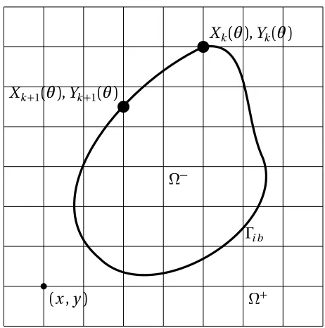
Figure 1.1Lagrangian Boundary Immersed in a Rectangular Eulerian Grid

1.1 Problem Formulation

The problem we are solving involves a closed box full of a viscous incompressible fluid with Drichlet Boundary conditions imposed on all four sides of the box. A massless elastic pressurised membrane is immersed in this fluid with a discontinuity in pressure. Figure 1.1 depicts a representative problem. Mathematically,

⇢

Å_{@ ~u}

@t + (u~.r~)u~

ã

+rp=µ u~_+f~ _(1.1)

r.u~₌0 (1.2)

~

f ₌

Z

i b

~

F_(X~_{) (x~ X}~_{)d s (1.3)} ~

F ₌ @

1.2. IMMERSED BOUNDARY AND INTERFACE METHODSCHAPTER 1. INTRODUCTION

d_X~

d t =

Z Z

⌦

~

u ₍x~ _X~_{)d x d y (1.5)}

Equations 1.1 and 1.2 are the incompressible Navier Stokes equations requiring that the divergence of velocity be zero.⇢,µ,u~ andp denote density, viscosity, velocity vector and pressure respectively.f~represents some source of an external force which in this case will be due to fluid structure interaction as shown in eqution 1.3. represents a delta function that will spread the force calculated in equation 1.4 to neighboring points on the eulerian grid and vice velocity. This force depends upon tensionT in the string. The immersed boundary points are advanced in time through an implicit update according to equation 1.5.

1.2 Immersed Boundary and Interface Methods

1.3. OVERVIEW CHAPTER 1. INTRODUCTION

approa

1.3 Overview

CHAPTER

2

NAVIER STOKES EQUATIONS

2.1 Overview

The incompressible Navier Stokes equations in two dimensions are reproduced below:

⇢

Å_{@ ~u}

@t + (u~.r~)u~

ã

+rp₌µ u~₊f~ (2.1)

.u~₌0 (2.2)

In equation 2.1,u~ ₌u₍x~,t₎is the velocity of the fluid and pressure is denoted byp ₌p₍x~,t₎

dependent upon positionx~_{= (}x,y₎. The coefficientsµand⇢are fluid viscosity and density respectively.Equation 2.1 can be rewritten in matrix form with⌫_=⇢µ as follows:

ñ_@u

@t

@v

@t

ô +

ñ

u@u

@x +v@@uy

u@v

@x +v@@vy

ô +

ñ_@p

@x

@p

@y

ô =⌫

ñ_@2_u

@x2 +@

2_u

@y2

@2_v

@x2 +@

2_v

@y2

ô +

ñ

f_x f_y

ô

2.2. MARKER AND CELL GRID CHAPTER 2. NAVIER STOKES EQUATIONS

Throughout this document,⇢₌1 and⌫is treated as the inverse of Reynold’s number. As alluded to earlier in Chapter 1, the forces f_x and f_y will be calculated through the interac-tion of elastic boundary and fluid using delta funcinterac-tions. The aim is to calculate the two dimensional velocity components and pressure over a rectangular grid. A discrete version of equation 2.3 is first implicitly solved and then pressure is calculated through a pressure projection method using equation 2.2.

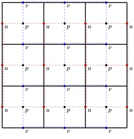
2.2 Marker and Cell Grid

The numerical discretization over a mesh is solved on the classic Marker and Cell (MAC) staggered grid. The three unknowns are both the velocity components as well as pressure at a given time and location. In solving the incompressible Navier Stokes equations, the horizontal velocity componentsu_i,j···u_m,n are located on the vertical walls of a given cell while the vertical velocity components are located on the horizontal walls in the same manner. As can be seen from Figure 2.1, solutions to the three unknown variables are obtained at three diffrent grids. This is further clarified in the next section where the spatial discretization of equations is discussed. In Figure 2.1, the dashed blue grid is used to obtain vertical component of velocity while the dashed red grid is for horizontal velocity. The pressure, as mentioned earlier, is calculated at the center of solid gridlines. The boundary conditions for such a grid become slightly complicated compared to a collocated grid and are explained in a later section.

2.3 Numerical Discretization

The x-component of equation 2.3 is discretized at time level n in the following manner.

u⇤ _un

t +

Å

u@u

@x +v

@u

@y

ãn+12

+ @p

@x

n 1₂

=⌫₂( u⇤ un_{) +}fn+12

2.3. NUMERICAL DISCRETIZATION CHAPTER 2. NAVIER STOKES EQUATIONS p p p p p p p p p v v v v v v v v v v v v u u u u u u u u u u u u

Figure 2.1Marker and Cell grid

The spatial discretization for the second term in equation eqn-2.4 depends upon the velocity at time level n as well as the previous time level n-1.

Å

u@u

@x +v

@u

@y

ãn+12

=3₂ ✓

u_in_,ju

n

i+1,j uin1,j

2 x +v

n s t a g

un

i,j+1 uin,j 1 2 y

◆

1 2

Ç

u_in_,j1u

n 1

i+1,j uin1,1j

2 x +v

n 1

s t a g

un 1

i,j+1 uin,j11 2 y

å (2.5)

The pressure term is discretized with a first order forward Euler method

@p @x n 1 2 =p n 1 2

i+1,j p n 1

2

i,j

x

un₌ u

n

i+1,j +2uni,j uin1,j

x2 +

un

i,j+1+2uin,j uin,j 1

y2

2.3. NUMERICAL DISCRETIZATION CHAPTER 2. NAVIER STOKES EQUATIONS

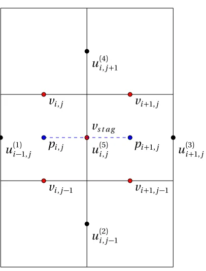
The calculation for velocity componentu requires and interpolation in equation 2.5 for

v_{s t a g}.

v_{s t a g =}1

4(vi,j +vi,j 1+vi+1,j+vi+1,j 1)

Figure 2.2 shows in detail the information required from adjoining cells to solve for velocity at a particular location. The idea is to plug in equations 2.6 and 2.5 to equation 2.4 and separate the terms to get an elliptic equation that is solved through linear solvers. After some rearrangement, 2.4 takes the form of equation 2.7.

u⇤

i+1,j ui⇤ 1,j

x2 +

Å ₂

x2+ 2

y2 2

⌫ t

ã

u⇤_{i,j +}u

⇤

i,j+1 ui⇤,j 1

y2

=_⌫2 0 @p

n 1₂ i+1,j p

n 1₂ i,j

x

1 A

+3⌫

✓

u_in_,ju

n

i+1,j uni 1,j

2 x +v

n s t

un

i,j+1 uin,j 1 2 y

◆

2⌫

Ç

un 1

i,j

un 1

i+1,j uin1,1j

2 x +v

n 1

s t

un 1

i,j+1 uin,j11 2 y

å

+u

n

i+1,j +2uni,j uni 1,j

x2 +

un

i,j+1+2uin,j uin,j 1

y2 +

Å_2⌫

t

ã

un_i,j+fx (2.7)

For comparison, the discrete Hemholtz Equation is reproduced below:

@2u

@x2+

@2u

@ y2+ u=b

Equation 2.7 is in the form of a discrete Hemholtz equation that can be solved through linear solvers using a five point stencil. For the purpose of this thesis, a multigrid solver DMGD9V[2]has been used which offers flexibility with boundary conditions.fx is a source

2.3. NUMERICAL DISCRETIZATION CHAPTER 2. NAVIER STOKES EQUATIONS

u(5)

i,j

u(1)

i 1,j ui(3+)1,j

u(4)

i,j+1

u(2)

i,j 1

vi,j 1

vi,j vi+1,j

vi+1,j 1

v_{s t a g}

pi,j pi+1,j

2.4. BOUNDARY CONDITIONS CHAPTER 2. NAVIER STOKES EQUATIONS

2.4 Boundary Conditions

Equation 2.7 is sufficient to calculate intermediate velocityu~⇤_{for all internal nodes in the} computational domain. However, the treatment of boundary conditions is more involved. Referring to equation 2.7 and figure 2.1, it is apparent that the five point stencil forui,1and

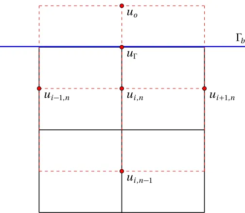
u_i,nmay require values outside the computational domain. In the case of Drichlet boundary conditions, some form of weighted average is needed to enforceu ₌u_b at the top and bottom. Similarly, if the boundary condition at the left and right of the computation domain is anything other than Drichlet (for example outflow), then calculations involvingv_{s t a g} will require values ofv on the left and right of the domain. The results in this thesis involve enforcement of a closed box and therefore only the Drichlet Boundary conditions are discussed. Figure 2.3 depicts the boundary at the top of the computational domain. Since the spatial discretization in equation 2.7 is second order, it is important to use consistent approximations at the boundary.

@u

@y =

ui,n uo

2 y =

1

2 x(ui,n+ui,n 1 2u )

@2u

@y2 =

u_{i,n 1} 2u_i,n+u_o

2 y =

4

3 x2(ui,n 1 3ui,n+2u )

(2.8)

2.5 Pressure Projection

According to Hemholtz Hodge Decomposition of the velocity field:

~

u⇤₌u~n+1

+ tr~ n+1

~

r.u~n+1

2.5. PRESSURE PROJECTION CHAPTER 2. NAVIER STOKES EQUATIONS

b

ui 1,n ui,n ui+1,n

u_o

u

u_{i,n 1}

Figure 2.3The MAC mesh near the Top boundary

The vector fieldu~⇤_{is projected on a divergence free vector fieldu~}n+1_{. Taking divergece of} both terms in equation 2.9 gives:

~

r.u~⇤

t =

n+1

@

@n =0

(2.10)

The discrete Laplace equation 2.10 is then solved over the pressure grid. The divergence of intermediate velocity calculated in the previous section is used as a source term for this equation. Equation 2.10 has been solved through the FISHPAK subroutine HWSCRT[4]. The discrete form is dependent upon ordering of the nodes and Figure 2.2 is consistent with the following discretization:

✓

i+1,j 2 i,j+ i 1,j

x2 +

i,j+1 2 i,j + i,j 1

y2

◆n+1 =

✓_u⇤

i+1,j ui⇤,j

x +

v⇤

i,j+1 vi⇤,j

y

◆Å ₁

t

2.5. PRESSURE PROJECTION CHAPTER 2. NAVIER STOKES EQUATIONS

Above equation is implicitly solved for with homogenous Neumann boundary conditions on all sides of the computation domain. Once is computed, the velocity is corrected through equation 2.9 to getu~n+1_{at the next time level. Brown et al[3]offered an accurate} projection method for correction to the pressure gradient:

rpn+12 ₌rpn 12 ₊r n+1 ⌫ t

2 r(

n+1 )

pn+12 ₌pn 12 ₊ n+1 ⌫

2 r~.u~⇤

(2.11)

CHAPTER

3

IMMERSED BOUNDARY METHOD

3.1 Introduction

This chapter deals with detailed information regarding the Immersed Boundry Method and its implementation. As alluded to earlier in Chapter 1, the method was developed by Peskin[12]to investigate complex geometries in heart valves that move within the fluid. A boundary is immersed in a fluid domain and the interaction between the fluid and the boundary is captured through Dirac Delta functions. The two basic assumptions are that the boundary is massless and that the fluid does not slip from the boundary. The fluid velocity is calculated at an eulerian grid as described in Chapter 2 while the velocity of immersed boundary is tracked over a lagrangian grid. The incompressible Navier Stokes equations are reproduced below for reference.

⇢

Å_{@ ~u}

@t + (u~.r~)u~

ã

3.2. LAGRANGIAN REPRESENTATION CHAPTER 3. IMMERSED BOUNDARY METHOD

The source termf~_{= (}fx,fy)is used to distibute the forces arising out when the fluid interacts

with the elastic boundary. The exact nature of these forces is derived later in this chapter.

3.2 Lagrangian Representation

The immersed boundary is represnted as a set of discrete pointsXk(✓),Yk(✓)where the

total number of discrete points isNb. Uppecase letters are used for the immersed boundary

to distinguish it from the original rectangular mesh on which the Navier Stokes Equations are solved. Therefore,_X~_{(✓,tn)is a vector function that defines the boundary as a function}

of arclengths₌r_o✓ and time t with respect to a reference configuration. The kth discrete point on the boundary is an approximation to₍X₍✓k,tn),Y(✓k,tn))where✓k is a reference

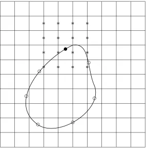
angle. Since the immersed boundary is assumed to be an elastic membrane, it is important to note that✓_k and in turn, the arclengths_k, is calculated on the basis of a reference config-uration. This line of reasoning will become more apparent in the next section where the forces are calculated. Figure 3.1 is a depiction of an arbitrary immersed boundary i b in a

rectangular grid. A reprsentative discrete pointXk(✓),Yk(✓)is also shown. Other possible

representations of the immersed boundary include level set functions[11]and cubic splines as introduced by Leveque and Li[8]in their work on Immersed Interface methods.

3.3 Representation of Forces

The forces in the special case of an immersed elastic membrane depend upon the tension in the immersed boundary. As mentioned earlier,s₌rno t✓ is the parametric coordinate. At a

given timetn, the tension is denoted byT(✓,tn). The unit tangent vector to the immersed

boundary is given by:

~

⌧₌ @ ~X/@s

3.3. REPRESENTATION OF FORCES CHAPTER 3. IMMERSED BOUNDARY METHOD

⌦

⌦+

Xk(✓),Yk(✓)

i b

(x,y₎ Xk+1(✓),Yk+1(✓)

Figure 3.1Immersed Boundary over a Rectangular Eulerian Grid

If we denote force applied by a section of immersed boundary from point a to point b by Rb

a F~(✓,tn)d s, then according to Newton’s third law:

0₌T⌧~

b

a

Z b

a

~

F₍✓,tn)d s

= Z b

a

Å _@

@s(T⌧~) F~

ã

d s

(3.3)

Keeping in mind thats₌r_o✓. Since a,b are arbitrary:

~

F ₌ @

@s(T⌧~) (3.4)

3.4. DISCRETE DELTA FUNCTIONS CHAPTER 3. IMMERSED BOUNDARY METHOD

Therefore,

T ₌

✓

@ ~X

@s 1

◆

(3.5)

The discretization of the force term will involve central differences. The terms T and⌧~

will be calculated atk ₊1₂ points and then the forcing term is calculated at the discrete immersed boundary points for equation 3.4

@ ~Xk

@s =

~

Xk+1 X~k

ro ✓

~

F_k=(Tk⌧~k) (Tk 1⌧~k 1) ro ✓

(3.6)

Equation 3.6 will give _F~ _{at the discrete immersed boundary points. It is important to}

note that since the immersed boundary is represented by discrete pointsXk,Yk, these

calculations will automatically result in a vector_F~_{= (Fx,Fy)in the x and y directions.}

3.4 Discrete Delta Functions

After the force at all imersed boundary points is calculated, the next logical step is to transfer this information to the eulerian grid on which the Navier Stokes equations are solved. The discrete dirac delta function is used to distribute the forces acting on the fluid at the eulerian points.. A variety of different delta functions are available in literature such as[6],[5],[9]. The force is distributed to eulerian points based on their distance from the lagrangian point being considered. If the distance of an eulerian point₍x,y₎from a langragian point

3.4. DISCRETE DELTA FUNCTIONS CHAPTER 3. IMMERSED BOUNDARY METHOD

⇤ ⇤ ⇤ ⇤

⇤ ⇤ ⇤ ⇤

⇤ ⇤ ⇤ ⇤

⇤ ⇤ ⇤ ⇤

Figure 3.2Force is spread from a Lagrangian point to Eulerian point

Newren[10].

h(x) =

8 < : 1

4h 1+c o s ⇡2hx |x|2h

0 _|x_| 2h (3.7)

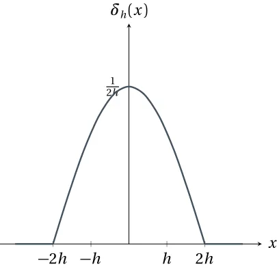
The delta function in 3.7 will transmit the forces to the nearest 16 points on the eulerian grid. Figure 3.3 shows the delta function in one dimension. In two dimensions, the delta function extends to:

(x,y_{) = (}x_{) (}y₎ (3.8)

The force distribution is accomplished by:

~

f ₌

Z

i b

~

3.5. LAGRANGIAN VELOCITY CHAPTER 3. IMMERSED BOUNDARY METHOD

2h h h 2h

1 2h

x

h(x)

Figure 3.3One dimensional delta function from equation 3.7. The function flattens out at a dis-tance 2hfrom the origin on both sides.

In discrete form, equation 3.9 takes the form of equation 3.10

~

f_{i,j =}

Nb

X

k

~

F_k(X_k,Y_{k) h(}x_i,j X_{k) h(}y_i,j Y_k) s_k (3.10)

Nb denotes the total number of lagrangian points. Equation 3.10 is directly added to the

Navier Stokes solver 2.7 and hence the effect of the immersed boundary is captured in calculating intermediate velocities. Once the velocity of the fluid is calculated, keeping in mind the physics of the problem, the next logical step is to calculate the velocity of the immersed boundary.

3.5 Lagrangian Velocity

3.6. MOVING BOUNDARY CHAPTER 3. IMMERSED BOUNDARY METHOD

lagrangian point. This is, in a way, a reversal of equation 3.10 which was used to distribute forces to the eulerian grid. This localised distribution in the case of forces and averaging in the case of velocity is depicted in figure 3.2. The velocity from nearest 16 points on the eulerian grid is averaged to get the velocity at the discrete immersed boundary point.

~

U₍X~_{) =}@ ~X @t =

Z Z

⌦

~

u₍x,y_{) h(}x~ X~₎dx~ (3.11) It is important to note that the vector notation throughout this document is used to de-note rectangular components both in discrete and continuous form._U~_(X~_{)denotes the}

lagrangian velocity of immersed boundary and⌦is the complete computational domain. In discrete form:

~

Uk = m

X

i n

X

j

~

ui,j h(xi,j Xk) h(yi,j Yk) x y (3.12)

One thing that needs to be mentioned here is that while distributing forces in equation 3.10 and collating velocities in equation 3.12, the form of the two dimensional discrete delta function is slightly different because velocities u and v are calculated at two diffrent grids in the Marker and Cell method as shown in figure 2.1.

3.6 Moving Boundary

An explicit way of moving the boundary is to use the forward Euler method. The new lagrangian location in this case as follows:

~

Xn+1

k X~kn

t =U~

n+1

k

~

Xn+1

k =X~kn+ tU~ n+1

k +O(h)

(3.13)

3.7. QUASI NEWTON METHOD CHAPTER 3. IMMERSED BOUNDARY METHOD

in[8]for Stokes flow and was later implemented for Navier Stokes equation in[6].

~

Xn+1

k =X~kn+

1 2 t U~

n

k (X~kn) +U~kn+1(X~kn+1) (3.14)

This means that the distance the immmersed boundary point moves is determined by the average of its velocity depending upon its previous location and its velocity depending upon the new location. This forms an implicit system of the form:

g_(X~n+1

) =X~n+1 X~n 1₂ t U~n(X~n) +U~n+1(X~n+1) (3.15) Normally, this equation will be solved through a Newton like method over a number of iterations to get tog_(X~n+1

) =0. The Hessian matrix for Newton Method would be:

H₍X~n+1

) =g0(X~n+1) =I 1₂ t U0(X~n+1) (3.16) A Newton Method, if applied to equation 3.16 will require that the three elliptic equations be solved at every iteration and then a₍2N_bx2N_b)system for the Hessian matrix be approx-imated through finite differences. The finite difference approximation will require that

~

U is evaluated a further 2N_b times. This will require a lot of work. This is the reason for implementing a quasi Newton method that will maintain an approximation to the Hessian matrix in the first iteration and will then be updated by a rank 2 update.

3.7 Quasi Newton Method

The exact Newton method aims to get the minimum of a function by calculating the point at which its gradient is zero. Suppose, we want to solve:

(P :₎ minf₍x₎

3.7. QUASI NEWTON METHOD CHAPTER 3. IMMERSED BOUNDARY METHOD

Atx ₌x¯,f₍x₎can be approximated by:

f₍x_)⇡h₍x_{) =}f ₍x¯_{) +r}f₍x¯₎T₍x x¯_{) +}1

2(x x¯)

t_H

(x¯₎₍x x¯₎

Which is the quadratic Taylor series expansion of f₍x₎atx₌x¯. Here_rf₍x₎is the gradient off ₍x₎andH₍x₎is the Hessian off₍x₎. This quadratic functionh₍x₎can be minimized by

rh₍x_{) =}0. Since the gradient ofh₍x₎is:

rh₍x_{) =r}f₍x¯_{) +}H₍x¯₎₍x x¯₎

rh₍x_{) =}0

x x¯₌ H 1₍x¯_)rf₍x¯₎

It has already been explained in the previous section that it is cost prohibitive to even approximate the Hessian matrix above. The motivation here is to show how any type of Newton’s Method can be adapted for equation 3.15. For any implementation of Newton’s method, the idea is to findx for which_rh₍x_{) =}0. In the case of equation 3.15, the term

g₍Xn+1_{)is treated asrh(x)to find the corresponding updates.The Rank 2 Quasi Newton} Method applied here aims to getg_(X~n+1_{) =0. Therefore, in the actual implementation, the} iteration is designed in the following manner:

Step 1:Make an initial guess at_X~n+1_{. SetI} =0

~

X[0]_=X~n

H=I

WhereHis the Hessian matrix andIis the 2Nbx2Nb identity matrix.

Step 2:Calculate_U~_(X~[I]_)usingX~[I]_=X~[0] _{for the first time. This will involve calculating}

velocity vectoru~[I]_{(intermediate velocity) and then interpolating.}

Step 3:Evaluateg_(X~[I]_{)using equation 3.15}

g_(X~I

) =X~[I] _X~n 1

2 t U~

n

3.8. VOLUME CONSERVATION CHAPTER 3. IMMERSED BOUNDARY METHOD

Step 4:

If _||g₍X~[I]

)||✏ Then X~n+1 =X~[I] where✏is some small tolerance and the present time step is over.

Else _X~[I]

=X~[I+1]_{, I}

=I₊1, Go toStep 2

For which the BFGS Rank-2 update needs to be calculated:

Rank-2 Update of Hessian Matrix

~

s₌Hg_(X~[I]

)

~

X[I+1]_=X~[I] _s~

~

y ₌g_(X~[I+1]_{) g(X~}[I]₎

~

b ₌Hs~

a₌1 y~

T_~b

~

sT_y~

H₌H₊~s₍as~t

+bT) ~bs~

T

~

sT_y~

Once the Hessian matrix is updated, the algorithm goes back toStep 2until the tolerance is met.

3.8 Volume Conservation

One of the biggest problems with any immersed boundary code is the preservation of volume (or area in two dimensions). For the membrane problem, at high Reynold’s numbers

3.8. VOLUME CONSERVATION CHAPTER 3. IMMERSED BOUNDARY METHOD

the velocity field in eulerian grid, does not act in the same predictable manner on the lagrangian grid. The choice of discreet divergence operator is also important here. For the divergence operator used in equation 2.10, the volume conservation problem is quite strong. The divergence free velocity on the eulerian grid does not remain divergence free after the interpolation to lagrangian grid.

Peskin and Printz[13]resolved this by modifying the divergence operator based on the choice of delta function used in the interpolation. The approach used in this work uses the method proposed by Newren[10]. The idea is that instead of modifying the divergence operators on the eulerian grid, the divergence free condition is applied to the lagrangian velocity itself. The continuous divergence equation on eulerian grid is:

ru~₌0 (3.17)

In weak integral form: _Z

⌦

rud V~ ₌0 (3.18)

The volume conservation inside the membrane denoted by⌦=_{from figure 3.1 is what we}

are interested in. Thus, _Z

⌦=

rud V~ ₌0 (3.19)

Applying the divergence theorem, Z

~

u.nd S~ ₌0 (3.20)

Wheren~is the outward normal to the immersed boundary. Since this last equation lives on the boundary,u~can be replaced by lagrangian velocity. In discrete form,

Nb

X

k

~

U.n~_k S_{k =}0 (3.21)

Sk is a representation of the arclength of the boundary. It is important to distinguish it

from s~k that was used in calculating forces because that depended upon the reference

3.8. VOLUME CONSERVATION CHAPTER 3. IMMERSED BOUNDARY METHOD

forces. Since the lagrangian points on the boundary do not remain equally spaced, an accurate way of enforcing equation 3.21 can be obtained by minimal effort. First,

~

t_k+= (X~k+1 X~k)

~

tk = (X~k X~k 1)

Sk+=||t~k+||

S_{k =||}t~_{k ||}

(3.22)

Where Sk+ and Sk measure the arclengths ahead of and behind a particular lagrangian

point respectively. Thus,

Sk=

1

2( Sk++ Sk ) (3.23)

A normalization of equation 3.22 will give localized tangent vectors just ahead of and behind the lagrangian point. The tangent vectors at lagrangian points will be a weighted average:

~ ⌧k+=

~

tk+

Sk+

~ ⌧k =

~

tk

Sk

~ ⌧k=

Sk+t~k + Sk t~k+

Sk++ Sk

(3.24)

Note, that the weighted tangent may not be normalized. Further, from the dot product rule:

~

n₌

Ç

n_k,x n_k,y

å =

Ç ˆ

⌧k,y

ˆ

⌧k,x

å

3.8. VOLUME CONSERVATION CHAPTER 3. IMMERSED BOUNDARY METHOD

Where ˆ⌧is the normalizef form of⌧~.Going back to equation 3.21, all terms have now been defined. Enforcing it requires:

M ₌

Nb

X

k

~

Uk.n~k Sk Nb

X

k

Sk

~

U_k=U~_{k Mn~k}

3.9. ALGORITHM CHAPTER 3. IMMERSED BOUNDARY METHOD

3.9 Algorithm

Since the computer program for this work requires that a number of different scripts to work together, it is pertinent to sketch a pseudocode for the overall algorithm. The details of calculations have already been explained.

Algorithm 1Immersed Boundary Algorithm Rank-2

1: Create a Rectangular Meshx~ ₍x,y₎

2: Store Lagrangian CoordinatesX~ ₍X₍✓),Y₍✓))

3: Setd t,⌫

4: Initializeu~,tn

5: Initializep:p⌦ >p⌦+

6: Averageu~ to lagrangian grid_U~

7: fortimet ₌0 :tn do

8: X~[I],n

=X~n

9: U~[I],n

=U~n

10: I ₌0 andH_(2Nbx2Nb)=I_(2Nbx2Nb) 11: whileg₍X~[I],n) ✏do

12: Solve Navier Stokes usingX[I],n,un,vn,pn

13: U[I+1] un+1,[I]

14: Use Rank-2 update:

15: X~[I+1] _{X~[I] +s}

16: H H₊Rank-2

17: I ₌I ₊1

18: end while

19: X~_b[I],n+1₌X~_b[I],n₊1₂₍U[I]_+U[0]₎

20: Un₌U[I]

21: n₌n₊1,t_n=t_n+d t

CHAPTER

4

NUMERICAL RESULTS

This chapter has been structured into three parts. The first part presents solutions for the membrane problem using the Immersed Boundary method employing the Quasi Newton method for updating the position of lagrangian points_X~_{b. The second approach uses two}

4.1. IBM WITH QUASI-NEWTON UPDATE CHAPTER 4. NUMERICAL RESULTS

time advancement because of the incompressibility of the fluid.

4.1 IBM with Quasi-Newton Update

Xb

Yb

-1 -0.5 0 0.5 1

-1 -0.8 -0.6 -0.4 -0.2 0 0.2 0.4 0.6 0.8 1

(a)t=0

Xb

Yb

-1 -0.5 0 0.5 1

-1 -0.8 -0.6 -0.4 -0.2 0 0.2 0.4 0.6 0.8 1

(b)t=0.12

Xb

Yb

-1 -0.5 0 0.5 1

-1 -0.8 -0.6 -0.4 -0.2 0 0.2 0.4 0.6 0.8 1

(c)t=0.24

Xb

Yb

-1 -0.5 0 0.5 1 -1 -0.8 -0.6 -0.4 -0.2 0 0.2 0.4 0.6 0.8 1

(d)t=0.36

Xb

Yb

-1 -0.5 0 0.5 1

-1 -0.8 -0.6 -0.4 -0.2 0 0.2 0.4 0.6 0.8 1

(e)t=0.73

Xb

Yb

-1 -0.5 0 0.5 1

-1 -0.8 -0.6 -0.4 -0.2 0 0.2 0.4 0.6 0.8 1

(f)t=0.97

4.2. COARSE LAGRANGIAN GRID CHAPTER 4. NUMERICAL RESULTS

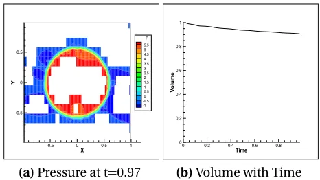
The solution is obtained on a 128x128 eulerian grid with Re=100. Figure 4.1 shows the membrane location at different time intervals.The number of lagrangian pointsN_b is 256. Generally, the number of points is taken such that the arclength between two adjacent points₍ s₎is_⇠h. The time interval t ish2_{at the start and is later increased. The time} interval t can become quite small while implicitly updating the immersed boundary. Figure 4.2a depicts the pressure within the domain. As expected, the discontinuity at the immersed boundary is smothered somewhat because of the use of discrete Dirac Delta functions. Further, figure 4.2b depicts the shrinking volume of the pressurised membrane. It is also apparent in figure 4.1f that the area of the circle is smaller than the initial ellipse.

X

Y

-0.5 0 0.5 1 -0.5 0 0.5 P 5.5 5 4.5 4 3.5 3 2.5 2 1.5 1 0.5 0 -0.5 -1

(a)Pressure at t=0.97

Time

Vo

lu

m

e

0 0.2 0.4 0.6 0.8

0 0.2 0.4 0.6 0.8 1

(b)Volume with Time

Figure 4.2Pressure and Volume loss

4.2 Coarse Lagrangian Grid

4.2. COARSE LAGRANGIAN GRID CHAPTER 4. NUMERICAL RESULTS

Xb

Yb

-1 -0.5 0 0.5 1 -1 -0.8 -0.6 -0.4 -0.2 0 0.2 0.4 0.6 0.8 1

(a)t=0

Xb

Yb

-1 -0.5 0 0.5 1

-1 -0.8 -0.6 -0.4 -0.2 0 0.2 0.4 0.6 0.8 1

(b)t=0.12

Xb

Yb

-1 -0.5 0 0.5 1

-1 -0.8 -0.6 -0.4 -0.2 0 0.2 0.4 0.6 0.8 1

(c)t=0.24

Xb

Yb

-1 -0.5 0 0.5 1

-1 -0.8 -0.6 -0.4 -0.2 0 0.2 0.4 0.6 0.8 1

(d)t=0.36

Xb

Yb

-1 -0.5 0 0.5 1

-1 -0.8 -0.6 -0.4 -0.2 0 0.2 0.4 0.6 0.8 1

(e)t=0.72

Xb

Yb

-1 -0.5 0 0.5 1

-1 -0.8 -0.6 -0.4 -0.2 0 0.2 0.4 0.6 0.8 1

(f)t=0.97

4.3. VOLUME CONSERVATION CHAPTER 4. NUMERICAL RESULTS

the membrane assumes the shape of a circle albeit with a reduced area. Figure 4.4b depicts this shrinking of the membrane over time.

X

Y

-0.5 0 0.5 1

-0.5 0 0.5 P 5.5 5 4.5 4 3.5 3 2.5 2 1.5 1 0.5 0 -0.5 -1

(a)Pressure at 4000

Projec-tions Time Vo lu m e

0 0.2 0.4 0.6 0.8 1

0 0.2 0.4 0.6 0.8 1

(b)Volume with Time

Figure 4.4Volume loss and Pressure

4.3 Volume Conservation

4.3. VOLUME CONSERVATION CHAPTER 4. NUMERICAL RESULTS

Xb

Yb

-1 -0.5 0 0.5 1

-1 -0.8 -0.6 -0.4 -0.2 0 0.2 0.4 0.6 0.8 1

(a)t=0

Xb

Yb

-1 -0.5 0 0.5 1

-1 -0.8 -0.6 -0.4 -0.2 0 0.2 0.4 0.6 0.8 1

(b)t=0.12

Xb

Yb

-1 -0.5 0 0.5 1

-1 -0.8 -0.6 -0.4 -0.2 0 0.2 0.4 0.6 0.8 1

(c)t=0.24

Xb

Yb

-1 -0.5 0 0.5 1

-1 -0.8 -0.6 -0.4 -0.2 0 0.2 0.4 0.6 0.8 1

(d)t=0.36

Xb

Yb

-1 -0.5 0 0.5 1

-1 -0.8 -0.6 -0.4 -0.2 0 0.2 0.4 0.6 0.8 1

(e)t=73

Xb

Yb

-1 -0.5 0 0.5 1 -1 -0.8 -0.6 -0.4 -0.2 0 0.2 0.4 0.6 0.8 1

(f)t=2.03

4.4. MESH REFINEMENT FOR LAGRANGIAN POINTSCHAPTER 4. NUMERICAL RESULTS

X

Y

-0.5 0 0.5 1 -0.5

0 0.5

P 5.5 5 4.5 4 3.5 3 2.5 2 1.5 1 0.5 0 -0.5 -1

(a)Pressure at t=0.97

Time

Vo

lu

m

e

0.2 0.4 0.6 0.8 0

0.2 0.4 0.6 0.8 1

(b)Volume with Time

Figure 4.6Volume loss after the same Time and Number of Projections as in the first Method

4.4 Mesh Refinement for Lagrangian Points

This section presents a mesh refinement analysis for the smaller set of Lagrangian points. Table 4.1 presents the levels of mesh refinement. In the absence of an accurate solution, the mesh refinement has been done by comparing the solution to a finer mesh ofn₌256. The parameters have been kept consistent to make this comparison. The last term in table 4.1 is the dense set of Lagrangian points. These calculations have been done atR e₌100.

Table 4.1Mesh Refinement Levels with Parameters

S.# h Time Step Nb 3Nb

1 2_/32 3.9_⇥10 3 _{22 66} 2 2/64 9.76_⇥10 4 _{44 132} 3 2/128 2.44⇥10 4 _{88 264} 4 2_/256 6.10_⇥10 5 _{176 528}

4.5. CONCLUSIONS AND FURTHER WORK CHAPTER 4. NUMERICAL RESULTS

Table 4.2Convergence Rates forXb andYb

S.# _||X_N X_256||2 Ratio _||Y_N Y_256||2 Ratio pE₁/E_3X pE₁/E_3Y

1 0.0546 – 0.0482 – – –

2 0.0274 1.9928 0.0272 1.7720 – –

3 0.0070 3.9033 0.0069 3.9570 2.7890 2.6480

meshes as expected. The order of accuracy is O(h) as expected at the immersed boundary.

4.5 Conclusions and Further Work

Figure 4.4b shows the reduction in volume when two different sets of Lagrangian points are used. It is clear that the second method moves much faster in time because the Quasi Newton Method has a smaller number of points to implicitly update. Hence, the reduction in volume at timet ₌0.97 for the method with cubic splines is much less than the method that does not use two different sets of lagrangian points. The volume reduction is depen-dent upon the number of projections performed. Volume reduction with Newren’s[10] proposed change makes the decrease in volume for the same number of projections almost nonexistent. A mathematically more robust immersed boundary method from a volume conservation point of view is the one proposed by Peskin_[13_].

Bibliography

[1] Colonius, T. & Taira, K. “The immersed boundary method: A projection approachs”.

Journal of Computational Physics225(2007), pp. 2118–2137.

[2] D., D. Z. “Matrix-dependent prolongations and restrictions in a blackbox multigrid solver.”Journal of Computational and Applied Mathematics33(1990), pp. 1–27.

[3] David L. Brown, R. C. & Minion, M. L. “Accurate Projection Methods for the Incom-pressible Navierâ ˘A¸SStokes Equations”.Journal of Computational Physics168(2001), pp. 464–499.

[4] John Adams, PaulL Swartzrauber and Roland Sweet.A Package of Fortran Subpro-grams for the Solution of Separable Elliptic Partial Differential Equations. Version 3.1.

[5] Lai, M.-C. & Peskin, C. S. “An Immersed Boundary Method with Formal Second-Order Accuracy and Reduced Numerical Viscosity”.Journal of Computational Physics160 (2000), pp. 705–719.

[6] Lee, L. & Leveque, R. J. “An Immersed Interface Method for Incompressible Navier– Stokes Equations”.SIAM Journal on Scientific Computing25.3 (2003), 832â ˘A¸S856.

[7] Leveque, R. J. & Li, Z. “The Immersed Interface Method for Elliptic Equations with Dis-continuous Coefficients And Singular Sources”.SIAM Journal on Numerical Analysis

31(1994), pp. 1019–1044.

[8] Leveque, R. J. & Li, Z. “Immersed Interface Methods for Stokes Flow with Elastic Boundaries or Surface Tension”.SIAM Journal on Scientific Computing18.3 (1997), pp. 709–735.

[9] Li, Z. & Lai, M.-C. “The Immersed Interface Method for the Navierâ ˘A¸SStokes Equations with Singular Forces”.Journal of Computational Physics171(2001), pp. 822–842.

[10] Newren, E. P. “Enhancing The Immersed Boundary Method: Stability, Volume Con-servation, and Implicit Solvers”. PhD thesis. The University of Utah, 2007.

[11] Osher, S. & Fedkiw, R. P. “Level Set Methods: An Overview and Some Recent Results”.

Journal of Computational Physics169(2001), pp. 463–502.

[12] Peskin, C. S. “Flow patterns around heart valves: A numerical method”.Journal of Computational Physics10(1972), pp. 252–271.