An Integrated Framework for Assessing the Dynamics of Population Growth and Climate Change for Urban Water Resources Management.

(1)

ABSTRACT

MASHHADI ALI, ALIREZA. An Integrated Framework for Assessing the Dynamics of Population Growth and Climate Change for Urban Water Resources Management. (Under the direction of Emily Z. Berglund.)

The management of water resources requires careful planning to balance water supply

and demand. Under increasing population growth and land use change through

urbaniza-tion, water shortages may become increasingly frequent, and climate change will alter the

availability and timing of water from expected levels. While long-term water supply planning

is conventionally based on projections of population growth, demands, and system capacity

under a stationary climate, the sustainability of water resources depends on the dynamic

interactions among the environmental, technological, and social characteristics of the water

system and local population. These interactions can cause supply-demand imbalances at

various temporal scales, and the response of consumers to water use regulations will impact

future water availability. Conventional approaches may rely on simple or linear assumptions

about water availability, population growth, and demand increases. To address the challenges

of water resources management and provide insight to system dynamics, new modeling is

needed to explicitly incorporate the feedbacks among these systems and their impacts on

water availability. The research described here develops a dynamic modeling approach to

simulate the supply-demand dynamics and feedbacks arising from urban growth dynamics,

consumer behaviors, and potential changes in climate and water demands. An agent-based

modeling (ABM) approach is developed to couple models of consumers and utility managers

with watershed and reservoir models. Households are represented as agents, and their water

use behaviors are represented as rules. A deterministic end use model is used to simulate

indoor demands, and landscaping demands are calculated based on irrigation requirements of

crops and behaviors of end users. A population growth model is used to simulate an increasing

number of household agents. A water utility manager agent enacts water use restrictions,

(2)

in precipitation and temperature. The integrated framework provides insight for water utility

operators and stakeholders about the interactions of management strategies, climate change,

population growth, and consumer behaviors, and the impact that these behaviors have on

long-term water supply sustainability. The framework is applied to the Falls Lake water supply

system in Raleigh, North Carolina to analyze the accuracy of the modeling framework and

assess sustainability of drought management plans. Accuracy is assessed using traditional

statistical metrics, and sustainability is measured using an index based on the satisfaction

or deficit of meeting water use demands that are exerted by a population. Low values for

traditional statistical metrics demonstrate that the ABM approach captures the dynamics of a

water system. This integrated framework provides an approach to create critical insights for

water utility operators and stakeholders about the impact of the interactions of management

strategies with climate change, population growth, and consumer behaviors on long-term

water supply sustainability. Results demonstrate the use of the ABM approach to project the

effectiveness of management policies for long-term planning, and based on the scenarios

tested in this research, a more restrictive drought policy can improve the sustainability of the

(3)

(4)

Urban Water Resources Management

by

Alireza Mashhadi Ali

A thesis submitted to the Graduate Faculty of North Carolina State University

in partial fulfillment of the requirements for the Degree of

Master of Science

Civil Engineering

Raleigh, North Carolina

2014

APPROVED BY:

Sankar Arumugam Kumar Mahinthakumar

(5)

DEDICATION

I dedicate this thesis to the three pillars of my life:

God and my parents.

Without you, my life would fall apart.

At each and every moment of life, talking to You, has given me strength. I might not know

where the life’s road takes me, but I believe I walk through this journey with You, God.

I would like to express my deepest gratude to my parents. Their support and unwavering

confidence in my ability helped me to achieve my academic dreams.

Mom, you have given me so much, thanks for your faith in me, and for teaching me that I

should never surrender.

Dad, you always told me to "trust yourself." I think I did. Thanks for inspiring my love for

engineering.

(6)

The author, born in Tehran, graduated in 2005 from a national high school for development of

exceptional talents in Iran. That autumn, Alireza Mashhadi Ali was awarded a full scholarship

by Amirkabir University of Technology to further his education in the major of Civil

Engineer-ing. Having finished his undergraduate study, he supplemented his career with working at

a construction company for two years. In fall of 2012, he admitted to North Carolina State

University to study Master of Science in Civil Engineering. After his graduation in August 2014,

(7)

ACKNOWLEDGEMENTS

This thesis would not have been possible without the support and encouragement that I

received from my advisor, Dr. Emily Berglund. I sincerely thank her for consistant efforts and

desire to keep me on track.

I would like also to thank my commitee members, Dr. Sankar Arumugam and Dr. Kumar

Mahinthakumar for serving in my defense committee despite their overwhelmingly busy

schedule.

Special thanks to the Dr. Ehsan Shafiee and other group members who helped and

(8)

LIST OF TABLES . . . vi

LIST OF FIGURES. . . vii

CHAPTER 1 INTRODUCTION . . . 1

CHAPTER 2 METHODOLOGY . . . 4

2.1 Agent-Based Modeling Framework . . . 6

2.1.1 Household agents . . . 6

2.1.2 Population growth model . . . 15

2.1.3 Water utility manager agent . . . 16

2.1.4 Water reservoir model . . . 17

2.2 Model Evaluation . . . 17

2.3 Sustainability Index . . . 19

2.3.1 Deficit . . . 19

2.3.2 Reliability . . . 19

2.3.3 Resilience . . . 20

2.3.4 Vulnerability . . . 20

2.3.5 Maximum deficit . . . 21

2.3.6 Sustainability index . . . 21

CHAPTER 3 RESULTS . . . 22

3.1 Application of ABM Framework for Raleigh, NC Water Supply . . . 22

3.1.1 Data for household agents . . . 23

3.1.2 Data for Falls Lake Reservoir . . . 28

3.1.3 Hydrologic data . . . 38

3.2 Model Evaluation Results . . . 38

3.3 Sustainability of Management Strategies for Climate Scenarios . . . 42

3.4 Stochasticity . . . 52

CHAPTER 4 DISCUSSION . . . 54

CHAPTER 5 SUMMARY & CONCLUSIONS . . . 56

CHAPTER 6 RECOMMENDATIONS . . . 58

BIBLIOGRAPHY . . . 60

APPENDIX . . . 62

(9)

LIST OF TABLES

Table 2.1 Water demand volume for household indoor end uses[Vic01] . . . 9

Table 2.2 Turf grass coefficients[MG87]. . . 13

Table 2.3 Watering frequency distribution[FS13]. . . 14

Table 2.4 Drought stages and level of response[BB11] . . . 15

Table 2.5 Drought stages and triggers . . . 16

Table 3.1 Raleigh population projections . . . 23

Table 3.2 Raleigh household average size (Raleigh Department of City Planning 2013 [CP13]) . . . 24

Table 3.3 Raleigh household size distribution (Raleigh Department of City Planning 2013[CP13]) . . . 24

Table 3.4 Distribution of build years for houses in Raleigh (Raleigh Department of City Planning 2013[CP13]) . . . 25

Table 3.5 Total land area for seven communities served by the City of Raleigh Water Utility (Raleigh Department of City Planning 2013[CP13]) . . . 25

Table 3.6 Raleigh land use allocation (Raleigh Department of City Planning 2013[CP13]) 26 Table 3.7 Allocation of residential zoning areas in Raleigh (Raleigh Department of City Planning 2013[CP13]) . . . 28

Table 3.8 Watering frequency distribution . . . 29

Table 3.9 Model evaluation criteria . . . 41

(10)

Figure 2.1 ABM framework. . . 7

Figure 2.2 Daily water demand for indoor end use appliances per person as reported by[Vic01] . . . 8

Figure 2.3 Distribution of leakage rates across households[DeO11] . . . 10

Figure 2.4 Daily water demand for indoor end use appliances per person as reported by[Vic01] . . . 11

Figure 2.5 Turf grass coefficient[MG87]. . . 14

Figure 3.1 Water allotments for Falls Lake in MSL (Mean Sea Level): flood storage, water Supply, water quality, and sediment storage. Figure based on data from the City of Raleigh Public Utilities Department (2011). . . 30

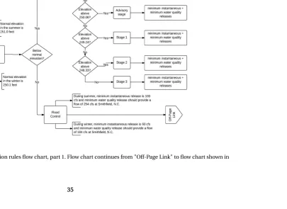
Figure 3.2 Water release operation rules flow chart, part 1. Flow chart continues from "Off-Page Link" to flow chart shown in Fig. 3.3. . . 35

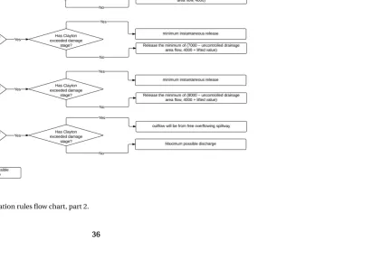
Figure 3.3 Water release operation rules flow chart, part 2. . . 36

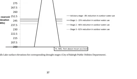
Figure 3.4 Falls Lake surface elevations for corresponding drought stages (City of Raleigh Public Utilities Department). . . 37

Figure 3.5 Historical inflow to the reservoir . . . 38

Figure 3.6 Outdoor water demand per capita per day . . . 39

Figure 3.7 Total water demand per capita per day . . . 39

Figure 3.8 Public water supply withdrawn from reservoir . . . 40

Figure 3.9 Water quality release . . . 40

Figure 3.10 Reservoir storage . . . 41

Figure 3.11 Future scenarios for inflow to the reservoir. . . 42

Figure 3.12 Monthly average of precipitation for three climate scenarios . . . 43

Figure 3.13 Monthly average of evapotranspiration for three climate scenarios . . . 43

Figure 3.14 Indoor water demand per capita per day for Scenario 1. Agents do not retrofit water appliances. . . 45

Figure 3.15 Indoor water demand per capita per day for Scenarios 2-6. Agents retrofit water appliances. . . 45

Figure 3.16 Outdoor demand for each management scenario and dry climate scenario . 46 Figure 3.17 Total demand for each management scenario and dry climate scenario . . . 47

Figure 3.18 Water supply for each management scenario and dry climate scenario . . . . 48

Figure 3.19 Water quality release for each management scenario and dry climate scenario 49 Figure 3.20 Reservoir storage for each management scenario and dry climate scenario . 50 Figure 3.21 Performance criteria and sustainability index values for management sce-narios, dry climate scenario . . . 51

Figure 3.22 Performance criteria and sustainability index values for management sce-narios, med climate scenario . . . 51

Figure 3.23 Performance criteria and sustainability index values for management sce-narios, wet climate scenario . . . 52

Figure 3.24 Reservoir storage . . . 53

Figure 3.25 Public water supply withdrawn from reservoir . . . 53

(11)

CHAPTER

1 INTRODUCTION

Urban water resources should be managed sustainably to achieve an appropriate balance

between water demand and supply. This balance is increasingly difficult to sustain as urban

areas increase in size, and precipitation decreases due to climate change. Traditionally, water

shortages are managed through supply management, which is based on the assumption that

economic growth generates new demands. Supply management does not control demand,

but increases the supply to meet demands. This approach leads to the depletion of freshwater

reserves and the construction of large infrastructure systems comprised of pipe networks and

pumping stations. Continuing to use a supply management approach is not feasible for many

utilities due to additional objectives and goals, such as greenhouse gas emissions, energy

(12)

emerged as a promising paradigm for sustainable management of water resources. Demand

management focuses on reducing demands through water pricing, educational campaigns,

incentives and rebates for water-saving technologies, regulations, and metering. Demand-side

strategies have the potential to significantly reduce demands, but they rely on changes in

human behavior, and the performance is impacted by social factors.

Management strategies are typically developed using linear projections of demands based

on population growth and evaluations of system capacity under a stationary climate and a

homogeneous population of consumers. The sustainability of water resources, however, may

be affected by the dynamic interactions among the environmental, technological, and social

characteristics of the water system and local population. The response of water consumers to

demand management strategies can affect the performance of management, and the dynamic

adoption of water-efficient appliances can impact the evolution of water availability. These

interactions can cause supply-demand imbalances that may not be predictable using

tradi-tional engineering models and assumptions of a stationary climate. Single-family residential

customers typically comprise the largest water demand sector in utilities across the United

States. Regional variations in climate across the country impact the relative consumption of

the single-family residential customer class and end use demand patterns.

This research develops a sociotechnical modeling approach to describe interactions among

the public, environmental resources, and engineering infrastructure and to simulate emerging

system-level properties of a water supply system. An agent-based modeling (ABM) approach is

developed to couple models of consumers and utility managers with watershed and reservoir

models. Households are represented as agents, and their water use behaviors are represented

as rules. A deterministic end use model is used to simulate indoor demands, and landscaping

demands are calculated based on irrigation requirements of crops and behaviors of end users.

A population growth model is used to simulate an increasing number of household agents. A

(13)

CHAPTER 1. INTRODUCTION

water storage. Water balance in a reservoir is simulated, and climate scenarios are used to test

the sensitivity of water availability to changes in precipitation and temperature. The integrated

framework provides insight for water utility operators and stakeholders about the interactions

of management strategies, climate change, population growth, and consumer behaviors, and

the impact that these behaviors have on long-term water supply sustainability.

The goal of this research is to develop a framework and approach for simulating the

emergence of water sustainability over a long-term horizon, rather than providing

short-term predictions. Results are generated using scenario analysis to provide insights about the

behavior of the system for a 20-year projection for alternative decision-making strategies.

Performance measures are used to evaluate resilience, reliability, the occurrence of deficits,

and sustainability and compare alternative water resources management strategies for climate

scenarios. The ABM framework is applied to simulate the water supply system of Raleigh,

North Carolina and to evaluate and compare alternative water shortage response plans and

(14)

2 METHODOLOGY

An ABM framework is developed to simulate urban water resources as a complex adaptive

system[Hol95]. A complex adaptive system is a system composed of a large network of decen-tralized actors without a cendecen-tralized controller and with the capability to adapt to a changing

environment. The collective actions of individual components give rise to complex,

hard-to-predict, and changing behaviors of the system ([Mit09],[MP09]). The complex behavior of the system at the macroscopic level, as it emerges from the collective actions of many interacting

components, can be simulated and described using an ABM approach. ABM is an approach for

creating a computer simulation in which entities and their interactions as they are identified

in the real system, are represented by software objects (agents) interacting with each other

(15)

CHAPTER 2. METHODOLOGY

Computer simulation improves tractability for scientific modeling in natural sciences and

provides capabilities to realistically represent the complexity of natural and human systems.

ABM provides modeling capabilities to directly represent individual actors as agents and avoids

the use of simplifying hypotheses about aggregated variables of the system. ABMs describe

individuals or agents as unique entities, which vary in characteristics, such as size, location,

and history. Agents are autonomous, and they act independently of one other to pursue

individual objectives. Agents also adapt their behavior or decisions based on their current state,

messages from agents, and the environment. ABM provides an approach to increase the level

of detail that can be included in simulation beyond the use of mathematical equations alone.

As a result, ABM facilitates the explicit study of individual influences and interactions and

provides an approach to study complex and seemingly unpredictable dynamics of a complex

system based on the actions of individuals. One criticism of ABM is that the complexity of

modeling may generate results that are not readily accessible, and, especially in the use as

a decision-support tool, there may be a tradeoff between the accuracy of a model and the

tractability of analysis.

ABM provides a useful methodology for studying water resources systems, because water

resources can consist of number of heterogeneous water consumers of different social

char-acteristics and technical elements such as water infrastructure components. The dynamic

interactions between social and technical elements can significantly impact the performance

of water resources management strategies. ABM has been developed for exploring the

influ-ence of human behaviors and decision-making on water resources systems. For example, ABM

frameworks were applied to study rules for the expansion of water infrastructure[Til05]and to model a population of customers with changing water demands ([Ath05];[Rix07];[Gal09]).

An ABM framework is developed here, and it is described in Section 2.1. The ABM

frame-work is used to simulate water use and water supply for a surface water system. Application

(16)

in Section 2.1, as it could be applied for any municipality. Details for the specific case study

are provided in Section 3. The metrics that are used to evaluate the accuracy of the model

for simulated historic data are described in Section 2.2. Metrics that are used to evaluate the

sustainability of management scenarios are described in Section 2.3. Again, these metrics are

described independent of specific case studies, and application is demonstrated in Chapter 3.

2.1 Agent-Based Modeling Framework

The framework is composed of subcomponents that capture various influential socio-technical

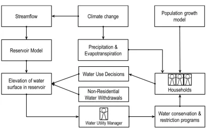
aspects of the water resources in a metropolitan area. Before describing the details of each of

the sub-models, it is important to explain the general structure of the overall model: the agents

and the technical models as the shared environment. The model includes household agents

and a water utility manager agent Fig. 2.1. Household agents withdraw water from the

reser-voir, and a hydrologic model is used to simulate runoff from the contributing watershed based

on climatological data. Household agents receive alerts from the water utility manger agent

about the level of water use restrictions, which are enacted when storage in the reservoir drops

below pre-defined stages. This model extends a framework that was developed to simulate

population growth, land use change, and water conservation for the City of Arlington, Texas

([Gia13];[KZ13]). The model is implemented in Java using MASON agent-based simulation libraries[Luk04].

2.1.1 Household agents

Households are simulated as agents, with properties and behavioral rules to simulate

household-level demands. Household size, house built year, and irrigated area are considered as

prop-erties, and rules are encoded to calculate indoor water use, adaptive outdoor water use,

(17)

2.1. AGENT-BASED MODELING FRAMEWORK CHAPTER 2. METHODOLOGY

Figure 2.1ABM framework.

agent is the sum of indoor end uses and the outdoor end use, described below.

Attributes can be initialized using historic information and projections. Household agents

are assigned the number of residents using demographic information and distribution of

household size based on U.S. Census Bureau.

2.1.1.1 Indoor end use demand model

An indoor end-use model is developed to describe the uses of water by a household at the

appliance level[Vic01] [Ken09]. Indoor water consumption in each household is disaggregated to eight end uses - showerhead, faucets, cloth washers, toilets, dishwashers, bathtub, leakage,

and others. Models for each end use are developed using a deterministic approach, which

assigns one value for each end use appliance to each household, and a probabilistic approach,

(18)

The end use model estimates the water use of each end-use per day per household as

the product of the water use rate of the end-use and the frequency of use (number of uses

per person per day), using volumes as shown in Table 2.1, as reported by[Vic01]. Daily water demands are multiplied by the number of days per month to obtain monthly demands. Daily

demands are calculated per person (Fig. 2.2) to explore the change in demands from pre-1950

to the present, due to the penetration of more water-efficient appliances. Water Sense

appli-ances provide the most water-efficient appliappli-ances, and they are adopted by agents after 2001

(the time of publication of the report). Household agents replace toilets, showerheads, faucets,

clothes washer, and washing machines with more efficient appliances after the appliance life

span has expired, and this changes the indoor water demand volume. The life span of each

appliance is simulated as 30 years. Each agent is assigned a set of appliances based on the

build year of its house. Each agent replaces appliances with more efficient appliances every

30 years. 0 5 10 15 20 25 30 35 40

Pre‐1950 1950s‐1980 1980‐1994 1994‐present WaterSense

Wat e r Use (gallon pe r da y per pe rso n )

Showerhead Toilet Faucets Dishwashers Cloth Washers

(19)

Table 2.1Water demand volume for household indoor end uses[Vic01]

Water Appliance/fixtures

Showerhead Toilet Faucet Dishwasher Cloth Washer

(gpm) (gpf ) (gpm) (gpl) (gpl)

Pre-1950 4.3 7 3.3 14 56

1950s-1980 4.3 5.5 3.3 14 56

1980-1994 1.8-2.7 3.5-4.5 1.8-2 9.5-14 43-51

1994-present 1.7 1.6 1-1.7 7-10.5 27-39

Water Sense 1.4 1 1 4.5 27

Frequency of Use 5.3 5.1 8.1 0.1 0.37

(20)

Leakage is also calculated as an end-use to represent water that is lost due to cracks in pipes

and leaky appliances. Instead of a deterministic end use calculation, as shown above, leakage

is estimated using a probabilistic distribution based on a study conducted in California in 2011

[DeO11]Fig. 2.3. It is assumed for this work that the California data can be applied for additional locations (e.g., Raleigh, North Carolina, as described in following sections). It is expected that

indoor uses across the country are similar for households of similar characteristics, such

as number of residents and house build year. Outdoor water use, on the other hand, varies

based on climate, and the California data is not used for outdoor water use approximations.

Leakage is not updated as homes are retrofitted, due to a lack of data to describe changes in

leakage rates with retrofits. The distribution of indoor water volume across all end uses, as

reported by[DeO11], is shown in Fig. 2.4. Leakage represents approximately 18% of indoor water consumption. 0% 10% 20% 30% 40% 50% 60% 70% 80% 90% 100% 0% 5% 10% 15% 20% 25% 30% 35% 40% 45% 50%

10 20 30 40 50 60 70 80 90 ₁₀₀ ₁₁₀ ₁₂₀ ₁₃₀ ₁₄₀ ₁₅₀ ₁₆₀ ₁₇₀ ₁₈₀ ₁₉₀ ₂₀₀

Mo re Cu m u lat ive Fr equency % of Hou se s Leakage Rate (gphd)

Relative frequency Cumulative Frequency

Figure 2.3Distribution of leakage rates across households[DeO11]

(21)

20%

19% 18%

18%

2% 2% 1%

Toilet

Shower

Faucet

Clothes Washer

Leaks

Other

Bath

Dish Washer

Figure 2.4Daily water demand for indoor end use appliances per person as reported by[Vic01]

standard deviation[DeO11]. Other end uses are those that simply do not fit neatly into another category. Like leakage end-use, the volume for other and bathing end uses are not updated

through retrofitting, due to a lack of data to describe changes in volume. End uses for bath

and other are calculated as follows.

B a t h=3.2±1 g p h d. (2.1)

O t h e r =7.8±2 g p h d. (2.2)

wheregphdstands for gallons per household per day, Bath is the volume of water used

for baths, and Other is the volume of water used for other end uses. Volumes are reported

(22)

2.1.1.2 Outdoor demand model

A significant portion of residential outdoor demand is used for garden watering. The following

approach calculates outdoor demand as a function of climatic data and water demands for

landscaping. Other outdoor demands, such as swimming pools and washing vehicles and

driveways, are neglected.

The water demands for landscape irrigation are calculated using a theoretical irrigation

model, which is based on a soil-water budget model. The theoretical irrigation requirement

(TIR) is calculated for each agent, or household, based on the area of land dedicated to each

plant type, evapotranspiration and precipitation data, efficiency of irrigation technologies,

and crop coefficient for each plant type.

T I R=0.624×E T_{o n e t}×

A E f f

×K_{c r o p} (2.3)

where

TIR=theoretical irrigation requirement (gal)

E To n e t=reference ETo (inches) minus effective rainfall (inches)

0.624=converts from inches of ETo net to gallons per square foot

A =irrigated area (square feet)

Eff =irrigation efficiency allowance

K_{c r o p} =crop coefficient

E T_{o n e t} is calculated as the difference between monthly evapotranspiration (E T_o) and

monthly rainfall.E T_{o n e t} is converted from inches to gallons per square foot using the

conver-sion factor 1 inch=0.624 gpsf. Household agents can use one of two types of turf grass, warm and cold, and monthly crop coefficients (Kc r o p) are shown in Table 2.2 and Fig. 2.5 for each

(23)

Table 2.2Turf grass coefficients[MG87]

Month Warm crop Cold crop

Jan 0.55 0.61

Feb 0.54 0.64

Mar 0.76 0.75

Apr 0.72 1.04

May 0.79 0.95

Jun 0.68 0.88

Jul 0.71 0.94

Aug 0.71 0.86

Sep 0.62 0.74

Oct 0.54 0.75

Nov 0.58 0.69

Dec 0.55 0.6

is 71% ([DeO11]).

Agents are assigned a behavioral factor to represent how often they water their lawn[FS13]. Eq. 2.4 is used to calculate the volume of water used for irrigation:

OW U = O I R×T I R (2.4)

whereOWUis outdoor water use that is exerted by an agent (gpd), andOIRis outdoor

irrigation ratio, which represents the fraction ofTIRthat an agent uses to water the lawn

(Table 2.3).

Household agents receive information from a water utility manager agent about the level

of outdoor water use restrictions, based on drought stages. Each stage is characterized by the

necessary restrictions, which must be implemented to preserve water supply. Households

reduce outdoor demands based on utility restrictions.

(24)

0

0.2

0.4

0.6

0.8

1 Jan Feb Mar Apr May Jun Jul Aug Sep Oct Nov Dec

Warm turfgrass

Cold turfgrass

Figure 2.5Turf grass coefficient[MG87]

Table 2.3Watering frequency distribution[FS13]

Watering Frequency Outdoor irrigation ratio

Never water 0

(25)

Table 2.4Drought stages and level of response[BB11]

Drought Stage Consumption Goal Level of Response (gpcpd) (Outdoor Restrictions)

PCM 65 No restrictions

Advisory Stage 60 Reduce water usage by 8% Stage 1 55 Reduce water usage by 15% Stage 2 35 Reduce water usage by 46% Stage 3 25 Reduce water usage by 62%

to alleviate demands in periods of water shortages or droughts. For the framework that is

implemented here, the level of response, or reduction of demands, for household agents are

calculated using the City of Raleigh’s Water Shortage Response Plan ([BB11]). According to the report, per capita per day consumption goals are set for each conservation stage, and

consumers should reduce their normal consumption to that amount. The ABM simulates

that each agent reduces its use by the percentage specified after a drought stage is enacted

(Table 2.4). For example, for Stage 2, residents should reduce their normal demand of 65

gallons per day to 35 gallons per day, and the reduction is 54%. Indoor end uses are not

affected by restrictions. PCM is Permanent Conservation Measures.

2.1.2 Population growth model

Population growth is simulated by increasing the number of household agents in the

pop-ulation at each time step, or month. Data for poppop-ulation growth are available through the

U.S. Census, and data about household sizes are available through specific utilities. The total

increase in population for each decade is divided by the average size of household at each

decade to obtain the total number of households. The total number of households is divided

(26)

Table 2.5Drought stages and triggers

Drought Stage Trigger Reverse Trigger (% WSSP) (% WSSP)

PCM N/A N/A

Advisory Stage <70% N/A Stage 1 <50% >=100% Stage 2 <30% >=70% Stage 3 <10% >=50%

agents that are added in the model. Households are populated based on the household size

distributions. The population increases linearly during each decade.

2.1.3 Water utility manager agent

The water utility manager is simulated as an agent that receives information about the surface

water elevation from the reservoir model at each monthly time step. Based on the reservoir

storage, the water utility manager agent defines the level of water restrictions: Permanent

Conservation Measures, Advisory Stage, and Drought Stages 1, 2, and 3. Restrictions are

enacted in response to decreasing reservoir storage.

The water utility manager agent uses triggers for enacting conservation stages and reverse

triggers to release conservation stages, as conditions return to normal. Triggers are based on

the storage in the reservoir for water supply, or water supply storage pool (WSSP). Storages

of less than 70%, less than 50%, less than 30%, and less than 10% correspond to triggers for

the Advisory Stage, Stage 1, Stage 2, and Stage 3, respectively. The reverse triggers for Stage 1,

Stage 2, and Stage 3 are 90%, 70%, and 50% of the reservoir storage, respectively. The drought

(27)

2.2. MODEL EVALUATION CHAPTER 2. METHODOLOGY

2.1.4 Water reservoir model

Reservoir storage is calculated on a monthly time-step using the continuity equation:

S_t = S_t₋₁+I_t−R_t −W S_t −S P_t +D e f_t (2.5)

whereSt is the volume of water stored in the reservoir at time stept;It is the monthly net

inflow to the reservoir (inflow plus precipitation over the lake surface minus evaporation from

the lake surface).R_t is the reservoir outflow (water quality releases) at time step t.W S_t is the

total water supply, which is the sum of the indoor and outdoor demands withdrawn from

reservoir at time step t,S P_t is reservoir spill, which is released when the water level within

the reservoir exceeds a pre-defined control elevation, andD e f_t is reservoir deficit or shortfall

whenSt =Sm i n.

At the beginning of each month, the reservoir model receives stream flow values based on

hydrologic data, the volume of water to be released based on operational rules, and the volume

of withdrawals from consumer agents. The storage at the end of the month is computed and

used as input for the water utility manager agent for selecting water use restrictions in the

subsequent month.

2.2 Model Evaluation

The model is evaluated to assess the accuracy in simulating the water supply system through

a set of statistical criteria. Models are evaluated using three evaluation statistics, described as

follows.

The absolute error is the magnitude of the difference between the exact value and the

(28)

value which is expressed as a percentage[Mor07].REvalue is calculated:

R E(%) =

Pn

i=1|(Oi−Si)|

Pn

i=1Oi

×100 (2.6)

where n is number of observations,Oi is observed value at timei, and Si is the value

simulated by the model at timei. Observed and simulated values are compared for demands,

release from a reservoir, and storage, as described in Chapter 3. A smaller value ofREindicates

better performance for the model.

Percent bias (PBIAS) measures the average tendency of the simulated data in exceeding or

under-estimated the observed data[Gup99].

P B I AS= Pn

i=1(Oi−Si)

Pn

i=1Oi

×100 (2.7)

The optimal value for this criterion is zero, and low-magnitude values indicate accurate

model simulation. Positive values indicate model underestimation bias, and negative values

indicate model overestimation bias.

The Nash-Sutcliffe efficiency (NSE) is a normalized statistic that determines the relative

magnitude of the residual variance compared to the observed data[NS70].NSEis computed as shown below:

N S E = 1−

Pn

i=1(Oi−Si)2

Pn

i=1(Oi−MO)2

×100 (2.8)

MO is the mean of observed data.NSEranges between -∞and 1.0 (1.0 inclusive), andNSE

equals 1.0 corresponds to perfect performance. Values between 0.0 and 1.0 are generally viewed

as acceptable levels of performance. Values less than 0.0 indicate that the mean observed value

(29)

2.3. SUSTAINABILITY INDEX CHAPTER 2. METHODOLOGY

2.3 Sustainability Index

Alternative management policies are evaluated using a sustainability index[SS10]. The analysis of a management policy focuses on system failure, defined as any output value in violation of

a performance threshold. Probability-based performance criteria include reliability, which

describes how often the system fails; resilience, which measures how quickly the system

comes back to a satisfactory state once a failure has occurred; vulnerability, which indicates

the significance of the likely consequences of failure; and maximum deficit.

2.3.1 Deficit

Demand (D e m a n dt) is calculated at each time step as the total public water demand that

will be withdrawn from the reservoir, and Supply (S u p p l y_t) is calculated as the volume of

water that the reservoir can deliver to the public.D e m a n d_t is the sum of residential and

non-residential demands on a monthly time step.S u p p l y_t is the amount of water that is

available in a reservoir to meet up to the volume that is demanded (D e m a n d_t), but it may

be less than that volume, if the water is not available in the reservoir. Therefore, a deficit (D_t)

is counted when the total water demand from reservoir is more than the available storage in

the reservoir; if the water demand is equal to water supply, deficit is zero (Dt =0). Therefore,

whenDt is greater than zero, the system fails.

D_t = 





D e m a n dt−1−S u p p l yt−1 ifD e m a n dt−1>S u p p l yt−1

0 ifD e m a n dt−1=S u p p l yt−1

(2.9)

2.3.2 Reliability

Water demand reliability is the probability that the available water supply meets the water

(30)

the fraction of time the water demand is fully supplied, or the number of timesDt =0, with

respect to the number of time steps simulated (nmonths).

R e l = No. of timesDt =0

n (2.10)

2.3.3 Resilience

Resilience is the capacity of a system to recover quickly from difficulties or period of failure

and to adapt to changing conditions. As water supply is threatened due to climate conditions,

which vary, resilience assesses the ability of water management policies to adapt to changing

conditions. Resilience is defined as the probability that a successful period follows a failure

period (the number of times thatD_t =0followsD_t >0) for all failure periods (the number of

timesD_t >0occurred). This statistic assesses the recovery of the system once it has failed:

R e s = No. of timesDt =0 followsDt >0

No. of timesDt >0 occured

(2.11)

2.3.4 Vulnerability

Vulnerability is the probable magnitude of deficits, if they occur ([Has82]). Vulnerability ex-presses the severity of failures, because even when the probability of failure is small, the

possible consequences of failure should be considered carefully. Vulnerability is the expected

value of deficits, or the sum of the deficits divided by the number of deficit periods, which is

the number of timesDt >0occurs. Vulnerability is expressed as a dimensionless number by

dividing the average annual deficits by the average annual water demand.

V u l =

Pt=n

t=0Dt

No. of timesDt>0 occured

(31)

2.3. SUSTAINABILITY INDEX CHAPTER 2. METHODOLOGY

2.3.5 Maximum deficit

The worst-case annual deficit is the maximum deficit.

M a x D e f = m a x(DAn n u a l)

Average Annual Water Demand (2.13)

2.3.6 Sustainability index

Finally, the Sustainability Index (SI)[SS10]represents the aggregate sustainability based on a combination of the performance criteria described above, including the reliability, the

resilience, the vulnerability, and the maximum deficit. The index is defined a geometric

average of the performance criteria.

(32)

3 RESULTS

3.1 Application of ABM Framework for Raleigh, NC

Water Supply

The ABM framework is applied to simulate the water supply system of Raleigh, North Carolina.

The city of Raleigh has a population of approximately 486,000 inhabitants over an area of

142.8 square miles in 2013, and the population of Raleigh is projected to increase to 848,000

inhabitants by the year 2032, as reported by the U.S. Census. The primary water supply source

for the city is Falls Lake, which is a man-made reservoir located on the upper Neuse River and

managed by U.S. Army Corps of Engineers. The Raleigh Water Utility provides water to Raleigh

(33)

3.1. APPLICATION OF ABM FRAMEWORK FOR RALEIGH, NC

WATER SUPPLY CHAPTER 3. RESULTS

Table 3.1Raleigh population projections

Year Population

1983 170,415 1993 244,430 2003 366,599 2013 529,840 2023 686,723 2033 848,365

Wendell, and Zebulon. Due to the population growth in the city of Raleigh and surrounding

communities served by Falls Lake over the last decade, the water storage in Falls Lake has

been increasingly stressed. Droughts were recorded in the years 2002, 2005, and 2007[Gol09].

3.1.1 Data for household agents

The ABM was initialized with a population of agents, where each agent represents one

house-hold.

N H_t = Pt

S_t (3.1)

whereN Ht is the number of households in yeart;Pt is the population in yeart; andSt is

the average size of households in yeart.

Household agents are assigned household size, or number of members, based on data

available through U.S. Census and Raleigh Department of City Planning (2013) (Table 3.3).

Using information in Table 3.4, agents are initialized with the build year for houses. Around

60% of houses are built before 1999.

A household agent is assigned a value for the area of land that it irrigates, which is based

on the amount of pervious area in a lot. Lot sizes are calculated using information in Table

(34)

Table 3.2Raleigh household average size (Raleigh Department of City Planning 2013[CP13])

Year Average household size

1980 2.67

1990 2.56

2000 2.54

2010 2.55

2020 2.55

2030 2.55

Table 3.3Raleigh household size distribution (Raleigh Department of City Planning 2013[CP13])

Household Size Percent of Population (%)

1-person household 32.8

4-person household 12

7-or-more-person household 1.2

(35)

Table 3.4Distribution of build years for houses in Raleigh (Raleigh Department of City Planning 2013[CP13])

2010 Housing Statistic Year Built

Housing, Median Year Built 1993

Built 1999 or Later 41.58% Built 1995 to 1998 7.52% Built 1990 to 1994 5.88% Built 1980 to 1989 14.97% Built 1970 to 1979 10.94% Built 1960 to 1969 8.37% Built 1950 to 1959 5.13% Built 1940 to 1949 2.61% Built 1939 or Earlier 3.01%

Table 3.5Total land area for seven communities served by the City of Raleigh Water Utility (Raleigh Department of City Planning 2013[CP13])

Year Land area (acres)

(36)

Table 3.6Raleigh land use allocation (Raleigh Department of City Planning 2013[CP13])

Land Use Percentage

Residential-Single Family 34.10% Residential - Apartment, Condominium 4.90% Residential - Townhouse, Multiplex 3.20%

Residential - Other 0.60%

Non-Residential 57.20%

TOTAL 100.00%

are served by the Raleigh Water Utility from 1980-2060 is shown in Table 3.5, based on historic

records and projections of urbanization (Raleigh Department of City Planning 2013). The land

area is distributed among several land use types, based on Raleigh land use allocation data for

the year 2013 (Table 3.6). The land use allocation remains constant over the simulation, as the

total land use dedicated to the service area increases. Due to lack of enough datat about land

use allocation over simulation time period, we assumed that non-residential area increases in

proportion to residential area.

At the beginning of the simulation, the lot size of each household is calculated based on

the area for the year of 1983 and the number of households:

T R A₁₉₈₃ = 0.428×T A₁₉₈₃ (3.2)

LS1983 =

T R A₁₉₈₃ N H1983

(3.3)

T R A₁983 is total residential area for the year 1983;T A₁983 is total area for the year 1983;

and 0.428 is the percentage of land use that is allocated to residential types of land use

(37)

in the year 1983, andN H₁983 is number of households in the year 1983.

Lot sizes are calculated for new household agents at each time step of the model. New

household agents are added to the population at each year, and the lot sizes for new agents

are determined for each decade, as follows. At the beginning of each decade, 42.8% of the

increased land area is divided by the number of new households for that decade to obtain the

lot size for new households.

I R A_t = 0.428×I A_t (3.4)

LSt =

I R A_t I N Ht

(3.5)

I R A_t is increased residential area for the yeart;I A_t is increased area for the yeart; 0.428 is

percentage of land use that is allocated to residential types of land use development, including

single family, apartment/condominium, townhouse/multiplex, other, and non-residential (shown in Table 3.6).LS_t is the lot sizes for new households that are added in the yeart, and

I N Ht is the number of households that are added in the yeart.

To determine the amount of area that is irrigated, the pervious areas for lots are calculated,

based on categories of residential areas. Residential area for the Raleigh area is divided into

ten groups, and each household is categorized as one type of residential area to determine

the pervious area of its lot size (Table 3.7). Pervious area is simulated as turf grass, and is used

to represent the irrigated area that is assigned to each household. The size of the pervious

area is calculated as follows.

P A = LS×P P (3.6)

PAis pervious area,LSis lot size for each household, andPP is percentage of pervious

area based on residential zone information in Table 3.7 (Raleigh Department of City Planning

2013).

(38)

Table 3.7Allocation of residential zoning areas in Raleigh (Raleigh Department of City Planning 2013[CP13])

Residential Zoning Density Pervious Area (%) (units/acre) (%)

Rural Residential 6.44 1.089 80

Residential 2 2.60 2 75

Manufactured Home 1.05 6 62

Special Residential 6 0.83 6 62

Special Residential 30 0.10 30 35

and these values are extracted from results of a survey of North Carolina residents about their

lawn-watering habits[FS13]. Household agents are assigned a value forOIRbased on the data reported in Table 13. Based on results reported in the survey[FS13], 60% of homes have warm turf grass, and 40% have cold turf grass.

3.1.2 Data for Falls Lake Reservoir

The Falls Lake reservoir provides Raleigh and its service area with water supply, which is

reserved in the Water Supply Storage Pool (WSSP) of the reservoir. The reservoir has multiple

purposes, and water is allocated for flood control, water quality, and sediment storage; leaving

only 42.3%, or 45,000 acre-feet of storage in Falls Lake for the WSSP storage Fig. 3.1.

(39)

Table 3.8Watering frequency distribution

Watering Frequency Percent Outdoor irrigation ratio

Never water 30.16% 0

Water new plants/stressed plants 42.31% 0.5 Water regularly or in absence of rain 27.53% 1

storage in the reservoir and implements water restrictions. The WSSP is calculated as:

W SS P = 0.423×(T S−SS) (3.7)

(40)

(41)

This storage supplies a service area population of approximately 500,000 which includes

the City of Raleigh and the Towns of Garner, Wake Forest, Rolesville, Knightdale, Wendell, and

Zebulon. Residential part comprises 56.6% of total demand of water supply for the Raleigh

service area, so as total residential water demand is calculated through the indoor and outdoor

models during simulation. Non-residential water demand is simulated as a non-adaptive

value, and the total demand as:

Total Demand = Residential Demand

0.566 (3.8)

Non-Residential Demand = (1−0.566)×Total Demand (3.9)

The City of Raleigh Public Utilities Department uses surface water from Falls Lake and

from the Swift Creek Lake system (Lakes Benson and Wheeler) as source of drinking water.

Falls Lake Reservoir which is located on the upper Neuse River and northwest of the City of

Raleigh has a surface area of over 12,500 acres and can provide Raleigh with up to 100 mgd

(peak day), 66.1 mgd (annual daily average) for the fifty-year reliable yield during the period of

record. The smaller Swift Creek lake system has a peak withdrawal rate of 20 mgd (peak day),

11.2 mgd (annual daily average) for the fifty-year reliable yield during the period of record. In

total, Falls Lake Reservoir and Swift Creek Lake provide 77.3 mgd (annual daily average) during

the period of record, and Falls Lake provides 66.1 mgd of that, or 85.5% of the total demand.

Because just Falls Lake is modeled as the surface water storage, demands are simulated as

85.5% of all calculated demands and are withdrawn from Falls Lake storage.

Water quality and flood control releases are simulated using operational rules that control

the release based on water level fluctuations in the reservoir on a daily basis and inflow

projections for subsequent days. The overall plan of operation for water control of Falls Lake

(42)

feet M.S.L, May through September, with April and October as transition periods. Flood control

storage space is reserved between elevations 250.1 and 264.0 feet M.S.L with surcharge storage

provided above the crest of the free-overflow spillway (from elevation 264.0 feet M.S.L up to

elevation 287.1 feet M.S.L). Conservation storage between elevations 250.1 and 236.5 feet M.S.L

is reserved for water supply as well as low flow and water quality control. Immediately below

the dam, a minimum instantaneous flow of approximately 60 CFS should be maintained

November through March and 100 CFS, April through October. Falls Lake also should be

operated to maintain water quality flow requirements in the Neuse River at Smithfield Rive

gage of 184 CFS and 254 CFS during the period of November through March and April through

October, respectively. Flood control and water quality rules are detailed in the following

sub-sections.

3.1.2.1 Operating Falls Lake for Flood Control

Storage of 220,880 acre-feet between elevations 250.1 and 264.0 feet M.S.L is reserved

exclu-sively for the detention of floodwaters. An additional 685,360 acre-feet of surcharge storage

exists above the free-overflow spillway between elevations 264.0 and 287.1 feet M.S.L. Falls

Lake releases are operated to produce non-damage stages in the downstream reaches of the

river whenever possible. Water is stored in the flood control space in Falls Lake whenever the

Clayton River gage exceeds a damage flow of approximately 7,000 CFS. Because of the

dis-tance from the dam to Clayton and the amount of uncontrolled drainage area above Clayton,

releases from the Falls Lake Dam may be terminated at the beginning of a storm to prevent

normal discharges from contributing substantially to the uncontrolled floodwaters at Clayton.

Therefore, discharges are halted (except for the minimum instantaneous release) whenever

the lake level is below elevation 264.0 feet M.S.L, and it is forecasted that runoff from the

storm may cause damaging flows in the lower Neuse River Basin. Once a storm has passed,

(43)

of 7000 CFS on the Clayton gage. The channel capacity below Falls Lake is 4000 to 8000 CFS.

Operational criteria for various flood situations are outlined as follows. Rules are summarized

as follows and in Fig. 3.2 and Fig. 3.3:

Lake elevation between 250.1 and 255.0 feet M.S.L.: if the flow from the uncontrolled

drainage area above Clayton is, or is forecasted to be, equal to or greater than 7000 CFS, the

reservoir outflow is released at 60 CFS or 100 CFS. If the flow from the uncontrolled drainage

area is less than 7,000 CFS, the reservoir release will be equal to the difference between 7,000

CFS and the flow from the uncontrolled drainage area, or 4,000 CFS, whichever is least.

Lake elevation between spillway crest 264.0 and 268.0 feet M.S.L.: if the flow from the

uncontrolled drainage area above Clayton is, or is forecasted to be equal to or greater than

8,000 CFS, the only outflow from the reservoir will be from overflowing spillway until the peak

flow at Clayton has occurred. After the peak at Clayton has occurred, releases from the conduit

should be the maximum possible, which is 8,000 CFS.

Lake elevation above 268.0 feet M.S.L.: The conduit will be fully open to pass maximum

(44)

3.1.2.2 Operating Falls Lake for Water quality

Minimum water quality flows in the lower Neuse River are established by the state of North

Carolina measured at the Smithfield River gage and should be 184 CFS and 254 CFS during

the period of November through March and April through October, respectively. A minimum

instantaneous flow of 60 or 100 CFS depending on the time of year will be maintained

imme-diately below the dam.

In the reservoir model, flows at locations downstream of the dam are represented as follows.

For water quality purposes, it is assumed that the flow that is released from the reservoir is

reaching the Clayton and Smithfield locations without any loss and at the same time step.

Therefore, the amount of flow at those gages is equal to the flow from reservoir. In flood

occasions, the flow at gages is calculated as the reservoir release added to the flow from the

flood area. A constant flow of 4000 CFS is assumed as runoff from the uncontrolled drainage

(45)

(46)

(47)

(48)

‐1000 0 1000 2000 3000 4000 5000 6000

1983 1985 1988 1990 1993 1996 1998 2001 2004 2006 2009 2012 Inflow (MSF)

Figure 3.5Historical inflow to the reservoir

3.1.3 Hydrologic data

Historic data is used for the inflow to the reservoir. Thirty years of monthly data are available

for the river that contributes flow to the reservoir, and are used as input values for the reservoir

simulation Fig. 3.5. As these monthly inflow data include evaporation losses, during low flow

month negative values are resulted.

3.2 Model Evaluation Results

The ABM simulates monthly values for the total demands in the population, reservoir storage,

and reservoir release. These values are compared to historical data for 1983-2013. Historical

inputs are used to simulate the demands, total withdraws, release, and storage for Falls Lake.

Outdoor demands are calculated Fig. 3.6, and Fig. 3.7 shows the total water usage per capita per

day for each month. Total demand decrease due to the effect of retrofitting indoor appliances.

Fig. 3.8 shows the total water withdrawal from Falls Lake reservoir for each month, which

includes the residential and non-residential demands. The value for the observed water

withdrawal from reservoir is plotted to compare with the simulated values. The model

(49)

3.2. MODEL EVALUATION RESULTS CHAPTER 3. RESULTS

0 50 100 150 200 250

1983 1987 1992 1997 2002 2007 2012

Outdoor demand (Gallon per capita

per day)

Figure 3.6Outdoor water demand per capita per day

0 50 100 150 200 250 300 350

1983 1987 1992 1997 2002 2007 2012

Total demand (Gallon per capita

per day)

(50)

decreased, due to droughts and increases in water prices. The model captures reactions of

consumers to decrease demands due to drought stages, but does not represent changes in

indoor water use that may have occurred due to droughts and pricing changes. This is a

limitation of the model that can be explored in further research.

0 5 10 15 20 25

1983 1987 1992 1997 2002 2007 2012

Water Supply (acre‐feet)

Th o u sa n d s Model Observed

Figure 3.8Public water supply withdrawn from reservoir

Fig. 3.9 depicts the water quality releases of reservoir throughout the simulation period.

The simulated and observed values are similar.

0 50 100 150 200 250 300

1983 1987 1992 1997 2002 2007 2012

Release

(acre‐feet)

Th o u sa n d s Model Observed

(51)

3.2. MODEL EVALUATION RESULTS CHAPTER 3. RESULTS

Table 3.9Model evaluation criteria

Criteria Storage Release Water Supply Simulation Simulation Simulation

NSE 0.33 0.70 -0.19

PBIAS (%) 2.98% 0.03% -1.37% RE (%) 13.69% 34.41% 20.63%

The performance of the model in predicting reservoir storage is shown in Fig. 3.10.

0 50 100 150 200 250 300 350

1983 1987 1992 1997 2002 2007 2012

Reservoir Storage (acre‐feet) Th o u sa n d s Model Observed

Figure 3.10Reservoir storage

The ability of the model to simulate water supply, reservoir release, and reservoir storage are

evaluated using the statistical metrics, RE, PBIAS, and NSE (3.9). The water release simulation

model shows accurate simulation, as demonstrated by low values of PBIAS, and NSE equal to

0.7. Simulation of water supply is not acceptable based on the value for NSE, but the relatively

low value of PBIAS indicates that average tendency of the simulated data is not significantly

larger or smaller than the observed values. Overall, the reservoir storage is predicted with a

medium level of performance, based on the metrics and NSE eauql to 0.33 which explains

(52)

3.3 Sustainability of Management Strategies

for Climate Scenarios

Future climate scenarios are constructed and used to evaluate the sustainability of six

man-agement scenarios. Future scenarios are simulated for 2013-2032 to explore the effectiveness

of policies.

To simulate runoff process for the future time period three climate scenarios are defined,

dry, medium, and wet climate. Inflows to the reservoir, monthly precipitation, and monthly

evapotranspiration are created for the three climate scenarios by sampling from the historic

data (Fig. 3.11 to Fig. 3.13). Scenarios are constructed by selecting 20 years of data from the

historic 30 years. The dry scenario is comprised of years with below average inflow values, the

medium scenario selects years with inflow values that are closest to the average values, and

the wet scenario is comprised of years with inflow values above the average.

0 500 1000 1500 2000

2013 2015 2017 2019 2021 2023 2025 2027 2029 2031

Inflow (CSF)

WET MED DRY

Figure 3.11Future scenarios for inflow to the reservoir.

Six management scenarios are defined by a set of rules for the actions of household agents

(53)

3.3. SUSTAINABILITY OF MANAGEMENT STRATEGIES

FOR CLIMATE SCENARIOS CHAPTER 3. RESULTS

0 10 20 30 40 50 60 70

2013 2015 2017 2019 2021 2023 2025 2027 2029 2031

Precipitation (Inch / Year)

WET MED DRY

Figure 3.12Monthly average of precipitation for three climate scenarios

0 10 20 30 40 50 60 70

2013 2015 2017 2019 2021 2023 2025 2027 2029 2031

Evapotranspiration

(Inch / Year)

WET MED DRY

(54)

Table 3.10Model evaluation criteria

Scenarios Triggers

1 NO Retrofitting NO Drought Restriction NA 2 Retrofitting NO Drought Restriction NA

3 Retrofitting Drought Restriction 60%-40%-20%-0% 4 Retrofitting Drought Restriction 70%-50%-30%-10% 5 Retrofitting Drought Restriction 80%-60%-40%-20% 6 Retrofitting Drought Restriction 90%-70%-50%-30%

water appliances. All household agents water lawns using the demand calculated by Eq.

2.3-Eq. 2.6, without reductions due to lawn watering habits. The water utility manager agent

does not enact drought stages. The second scenario is created to investigate the impact of

retrofitting water appliances on residential water demand without any drought restrictions.

Scenarios 3-6 analyze the impact of drought restrictions on sustainability by testing various

settings for triggers (3.10).

Management scenarios are analyzed for three defined climate scenarios. Indoor demands

are not affected by drought restrictions and differ when household agents retrofit water

appliances (Scenarios 2-6). Fig. 3.14 and Fig. 3.15 show average indoor demand for agents

that do not retrofit and do retrofit appliances, respectively. Though households do not replace

their water appliances with more efficient ones, the average demand decreases, because as

more households with more water efficient appliances are added to the community of agents,

they reduce the average indoor demand (Fig. 3.14). Fig. 3.15 shows that each time step there is

a small drop in demand, due to retrofits.

Results for each management scenario and the dry climate scenario are shown in Fig. 3.16

to Fig. 3.21. Most notably, Scenario 6 shows that the water supply does not reach zero in

(55)

0 10 20 30 40 50 60 70 80 90 100

1983 1987 1992 1997 2002 2007 2012 2017 2022 2027 2032

Indoor demand

(Gallon per capita per day)

Figure 3.14Indoor water demand per capita per day for Scenario 1. Agents do not retrofit water appliances. 0 10 20 30 40 50 60 70 80 90 100

1983 1987 1992 1997 2002 2007 2012 2017 2022 2027 2032

Indoor demand

(Gallon per capita

per day)

(56)

decreasing reservoir levels, water demands are reduced and the water supply is sustained.

Therefore, water is available in the reservoir for subsequent time steps.

Figure 3.16Outdoor demand for each management scenario and dry climate scenario

The base case scenario overestimates residential water use, when compared to historic

data and evaluated based on its sustainability index, which is around 40%. Fig. 3.21 shows the

results for the six management scenarios. Results show that as retrofitting and drought

restric-tions are enacted, (1) maximum deficit decreases; (2) vulnerability decreases; (3) resilience

(57)

(58)

(59)

(60)

(61)

water appliances improves sustainability and all performance measures. Scenarios 5 and 6

improve the sustainability index to nearly 80%, because the vulnerability and max deficit

decreases due to the reactive triggers.

0% 20% 40% 60% 80% 100%

1 2 3 4 5 6

Per fo rma nce C rit e ria & Su st ai na bi lit y In de x (% ) Scenarios

Reliability Resilience Vulnerability Max Deficit Sustainability Index

Figure 3.21Performance criteria and sustainability index values for management scenarios, dry climate scenario

For the med climate scenario, the sustainability index increases across the Scenarios

(Fig. 3.22), through Scenario 6 increases the value of the index compared to Scenario 5 by a

small value. 0% 20% 40% 60% 80% 100%

1 2 3 4 5 6

P e rfor mance Crit er ia & Su st ai nabi lit y Index (% ) Scenarios

(62)

For the wet scenario, there is little change in the value of the sustainability index or other

metrics across the management scenarios (Fig. 3.23). For the wet climate, there is little stress

on the reservoir and water supply system, and the performance criteria are at optimal values

for all management scenarios.

0% 20% 40% 60% 80% 100%

1 2 3 4 5 6

Pe rf o rm an ce Cr iter ia & Sus ta inabil ity Index (%) Scenarios

Figure 3.23Performance criteria and sustainability index values for management scenarios, wet climate scenario

3.4 Stochasticity

Stochasticity in the model is shown in the result for the reservoir storage, public water supply,

and reservoir releases (Fig. 3.24 to Fig. 3.26). Each model was executed for 30 random trials,

but results show little variation due to little randomness in the model initialization and few

stochastic processes. One source of stochasticity is in the calculation of the bath, leakage, and

other end uses and another one is a stochastic process for the assignment of lawn watering

behaviors. Because the population is large, this stochasticity does not significantly affect the

results. Water use behaviors can be more realistically represented in future research to better

(63)

3.4. STOCHASTICITY CHAPTER 3. RESULTS 0 50 100 150 200 250 300

1983 1987 1992 1997 2002 2007 2012 2017 2022 2027 2032

Reservoir Storage (acre‐feet)

Th o u san d s Mean MAX MIN

Figure 3.24Reservoir storage

0 5 10 15 20 25

1983 1987 1992 1997 2002 2007 2012 2017 2022 2027 2032

Water Supply

(acre‐feet)

Th o u sand s Mean MAX MIN

Figure 3.25Public water supply withdrawn from reservoir

0 50 100 150 200 250 300

1983 1987 1992 1997 2002 2007 2012 2017 2022 2027 2032

Release (acre‐feet) Th o u san d s Mean MAX MIN