Intelligent Load Monitoring in Beam Structures

Abstract

Li, Junping Intelligent load monitoring in beam structures. (Under the direction of Dr. F. G. Yuan.)

A robust approach for identifying impact load location and impact force history in beam structures is presented in this thesis. Beam strain transients propagating from the impact site can be inverted to yield the impact location and force history. Solving the inverse problem consists of three parts: a transient wave model, an impact location determination, and then an impact history identification. The classical Euler-Bernoulli beam theory (EBT) is used to obtain the dynamic models of a simply-supported beam.

INTELLIGENT LOAD MONITORING IN BEAM

STRUCTURES

By

Junping Li

A thesis submitted to the Graduate Faculty of North Carolina State University

in partial fulfillment of the requirements for the Degree of

Master of Science

Mechanical Engineering

Raleigh

2002

Approved by:

_________________________ _________________________ Dr. Kara Peters Dr. Fen Wu

__________________________ Dr. Fuh G. Yuan

Biography

Acknowledgements

First of all, I would like to thank Dr. F. G. Yuan for suggesting the following work and serving as my graduate advisor over the past more than two years. I appreciate very much his warm guidance and enthusiastic encouragement throughout the work. Especially, his insight into research topic and his insistence of pursuing perfect in research impress me greatly. I would also like to thank Dr. Kara Peters and Dr. Fen Wu for providing helpful advice in completing this research. Special thank goes to Dr. Gregory D. Buckner, who give me a deep understanding of Radial Basis Function neural network about how to set the parameters and train the networks. Without his help, much longer time could be needed to complete this work.

I would also like to express my thanks to Dr. Shaorui Yang, who has given me lots of help in understanding the principles of the beam theory, and to Mr. Lei Wang, who help me to utilize the Wavelet Toolbox in Matlab. Also, thanks go to all the members in our research group and my roommates for their care and help. The friendship with them makes my life at Raleigh easier and more colorful.

Thanks also go to my friends who showed strong confidence in my ability and consistent encouragement. Hong Yang, and Lei Wan are among them. Especially, my deepest appreciation goes to my friend, Xin Wang, who was there wherever I needed.

Finally, I should thank my father, mother and brothers. Without their strong support, I could never reach this joyful moment. I dedicate this thesis to them.

Table of Contents

Page

List of Tables…….………...VI List of Figures…….……..………..…VII

1:Introduction……...……..………..….1

1.1Literature Review………...1

1.2Proposed Method………...6

2: Flexural Waves in a Beam………...…………..………….……….….8

2.1 Governing Equation of Bernoulli-Euler Theory.……..……….8

2.2 Finite Element Formulation Based on EBT……….10

2.3 Beam Transient wave Analysis Based on State Variable Approach……...…12

2.4 Comparisons of Solutions from Proposed Method and ANSYS…………...17

2.4.1 Stability and Accuracy………20

3: Determination of Impact Location Using Continuous Wavelet Transform (CWT)………...26

3.1 Continuous Wavelet Transform………...26

3.2 Time-Frequency Analysis of Wave Propagation……….30

3.3 Identification of the Impact Location………..32

3.4 Numerical Results………34

3.4.1 Case 1: Triangular-shaped Impact Load………..35

3.4.2 Case 2: Half-sine Impact Load..………..37

3.4.3 Case 3: Five-peak Impact Load………...38

4: Radial Basis Function Neural Networks…………..……….………59

4.1 RBFN Networks………..59

4.3.1 De-noising the Strain Measurements Using Discrete wavelet

Transform………...66

4.3.2 Normalizing the inputs……….70

4.3 Numerical Results..….……….70

4.3.1 Case 1: Triangular-shaped Impact Load………..71

4.3.2 Case 2: Half-sine Shape Impact Load………..72

4.3.3 Case 3: Five-peak Impact Load.………..72

5: Discussion and Conclusions………….………….………....104

Appendix A: Timoshenko Beam Theory ( TBT)…..……….…..106

A.1 Governing Equation………..106

A.2 Dispersion Relation for the Timoshenko Beam and Euler-Bernoulli Beam.109 Appendix B: Calculation of Exponential MatrixΦ and Γ………...…..114

List of Tables

Page

Table. 2.1 The dimensions and material constants of the Al-6061 beam………18 Table. 3.1 Arrival times selected from measurements without noise and the

locations estimated for triangular-shaped impact load……….……...36 Table. 3.2 Arrival times selected from measurements with SNR=10 and the

locations estimated for triangular-shaped impact load………...………37 Table. 3.3 Arrival times selected from measurements without noise and the

locations estimated for half-sine impact load………....….………37 Table. 3.4 Arrival times selected from measurements with SNR=10 and the

locations estimated for half-sine impact load………..………38 Table. 3.5 Arrival times selected from measurements without noise and the

locations estimated for five-peak impact load………….………38 Table. 3.6 Arrival times selected from measurements with SNR=10 and the

locations estimated for five-peak impact load.………39 Table. 4.1 The values of weights after 2000 iterations for triangular-shaped

impact load at two sensor locations………...………..73 Table. 4.2 The values of weights after 1000 iterations for triangular-shaped

impact load at two sensor locations………...………..74 Table. 4.3 The values of weights after 2000 iteration for half-sine impact load

at two sensor locations………..………..75 Table. 4.4 The values of weights after 1000 iteration for half-sine impact load

at two sensor locations………..………..76 Table. 4.5 The values of weights after 2000 iteration for five-peak impact load

List of Figures

Page

Fig. 2.1 Euler-Bernoulli beam element subjected load………...9

Fig. 2.2 A Euler beam element………..10

Fig. 2.3 Beam subjected to an impact load………...13

Fig. 2.4 The dispersion relations of group velocity for EBT and TBT……….18

Fig. 2.5 Triangular-shaped load history and its frequency spectrum………22

Fig. 2.6 Comparison of transverse displacement from ANSYS and present method.……….23

Fig. 2.7 Five-peak load history and its frequency spectrum……….24

Fig. 2.8 Comparison of transverse displacement from ANSYS and present method.……….25

Fig. 3.1 Gabor function and its Fourier transform………29

Fig. 3.2 Estimation of the impact location………33

Fig. 3.3 The simulated strain measurements without noise when the beam is subjected to the triangular-shaped impact load………....40

Fig. 3.4 Contour plot of the time-frequency distribution of the WT for the strain without noise when the beam is subjected to the triangular-shaped impact load……….……..41

Fig. 3.5 The magnitude of the WT for f =1.45 kHz without noise when the beam is subjected to the triangular-shaped impact load………..42

Fig. 3.6 The simulated strain measurements with SNR=10 when the beam is subjected to the triangular-shaped impact load……….…..43

Fig. 3.8 The magnitude of the WT for f =1.45 kHz with SNR=10 when the

beam is subjected to the triangular-shaped impact load………....…..45 Fig. 3.9 Half-sine load history and its frequency spectrum………..…46 Fig. 3.10 The simulated strain measurements without noise when the beam is

subjected to the half-sine impact load……….47 Fig. 3.11 Contour plot of the time-frequency distribution of the WT for the strain

without noise when the beam is subjected to the half-sine impact load……..48 Fig. 3.12 The magnitude of the WT for f =2 kHz without noise when the beam

is subjected to the half-sine impact load……….…….49 Fig. 3.13 The simulated strain measurements with SNR=10 when the beam is

subjected to the half-sine impact load……….50 Fig. 3.14 Contour plot of the time-frequency distribution of the WT for the strain

with SNR=10 when the beam is subjected to the half-sine impact load….…51 Fig. 3.15 The magnitude of the WT for f =2 kHz with SNR=10 when the beam

is subjected to the half-sine impact load……….………....52 Fig. 3.16 The simulated strain measurements without noise when the beam is

subjected to the five-peak impact load…………..………..53 Fig. 3.17 Contour plot of the time-frequency distribution of the WT for the strain

without noise when the beam is subjected to the five-peak impact load…….54 Fig. 3.18 The magnitude of the WT for f =10 kHz without noise when the

beam is subjected to the five-peak impact load……….…..55 Fig. 3.19 The simulated strain measurements with SNR=10 when the beam is

subjected to the five-peak impact load………..…...……….……..56 Fig. 3.20 Contour plot of the time-frequency distribution of the WT for the strain

Fig. 4.1 ANN supervised learning processing……….………..60

Fig. 4.2 RBFN networks architecture………..….………….60

Fig. 4.3 RBFN networks for dynamic load identification……….…………....64

Fig. 4.4 1D-DWT decomposition tree………...68

Fig. 4.5 Daubechies scaling function and wavelet function………..79

Fig. 4.6 (a) Strain measurement without white noise at x₁ =99.375cm (b) Comparison of NN predicted impact load with the actual one without white noise atx₁ =99.375cm………80

Fig. 4.7 (a) Strain measurement with white noise SNR=20 at x₁ =99.375cm (b) Comparison of NN predicted impact load with the actual one with white noise SNR=20 atx₁ =99.375cm………..……...………81

Fig. 4.8 (a) Strain measurement with white noise SNR=10 at x₁ =99.375cm (b) Comparison of NN predicted impact load with the actual one with white noise SNR=10 atx₁ =99.375cm………..……...………82

Fig. 4.9 (a) Strain measurement after de-noising SNR=10 at x₁ =99.375cm (b) Comparison of NN predicted impact load with the actual one after de-noising SNR=10 atx₁ =99.375cm………...……...………83

Fig. 4.10 (a) Strain measurement without white noise at x₂ =138.125cm (b) Comparison of NN predicted impact load with the actual one without white noise atx₂ =138.125cm………84

Fig. 4.11 (a) Strain measurement with white noise SNR=20 at x₂ =138.125cm (b) Comparison of NN predicted impact load with the actual one with white noise SNR=20 atx₂ =138.125cm...………..…………...………..85

Fig. 4.13 (a) Strain measurement after de-noising SNR=10 at x₂ =138.125cm

(b) Comparison of NN predicted impact load with the actual one after

de-noising SNR=10 atx₂ =138.125cm………...……….……87 Fig. 4.14 (a) Strain measurement without white noise at x₁ =99.375cm

(b) Comparison of NN predicted impact load with the actual one without white noise atx₁ =99.375cm………88 Fig. 4.15 (a) Strain measurement with white noise SNR=20 at x₁ =99.375cm

(b) Comparison of NN predicted impact load with the actual one with

white noise SNR=20 atx₁ =99.375cm………...………..89 Fig. 4.16 (a) Strain measurement with white noise SNR=10 at x₁ =99.375cm

(b) Comparison of NN predicted impact load with the actual one with

white noise SNR=10 atx₁ =99.375cm………..……...………90 Fig. 4.17 (a) Strain measurement after de-noising SNR=10 at x₁ =99.375cm

(b) Comparison of NN predicted impact load with the actual one after

de-noising SNR=10 atx₁ =99.375cm………...……...………91 Fig. 4.18 (a) Strain measurement without white noise at x₂ =138.125cm

(b) Comparison of NN predicted impact load with the actual one without white noise atx2 =138.125cm………..92

Fig. 4.19 (a) Strain measurement with white noise SNR=20 at x2 =138.125cm

(b) Comparison of NN predicted impact load with the actual one with

white noise SNR=20 atx₂ =138.125cm..………...……….93 Fig. 4.20 (a) Strain measurement with white noise SNR=10 at x₂ =138.125cm

(b) Comparison of NN predicted impact load with the actual one with

de-noising SNR=10 atx₂ =138.125cm..………...……...………95 Fig. 4.22 (a) Strain measurement without white noise at x₁ =99.375cm

(b) Comparison of NN predicted impact load with the actual one without white noise atx₁ =99.375cm………96 Fig. 4.23 (a) Strain measurement with white noise SNR=20 at x₁ =99.375cm

(b) Comparison of NN predicted impact load with the actual one with

white noise SNR=20 atx₁ =99.375cm…………..………...………97 Fig. 4.24 (a) Strain measurement with white noise SNR=10 at x₁ =99.375cm

(b) Comparison of NN predicted impact load with the actual one with

white noise SNR=10 atx₁ =99.375cm………..……...………98 Fig. 4.25 (a) Strain measurement after de-noising SNR=10 at x₁ =99.375cm

(b) Comparison of NN predicted impact load with the actual one after

de-noising SNR=10 atx₁ =99.375cm………...……...………99 Fig. 4.26 (a) Strain measurement without white noise at x₂ =138.125cm

(b) Comparison of NN predicted impact load with the actual one without white noise atx₂ =138.125cm……….…..…….100 Fig. 4.27 (a) Strain measurement with white noise SNR=20 at x2 =138.125cm

(b) Comparison of NN predicted impact load with the actual one with

white noise SNR=20 atx2 =138.125cm………...………...……...101

Fig. 4.28 (a) Strain measurement with white noise SNR=10 at x₂ =138.125cm

(b) Comparison of NN predicted impact load with the actual one with

white noise SNR=10 atx₂ =138.125cm..………..……...……..102 Fig. 4.29 (a) Strain measurement after de-noising SNR=10 at x₂ =138.125cm

(b) Comparison of NN predicted impact load with the actual one after

Chapter 1 Introduction

1.1 Literature Review

In the study of the response of structures using structural models, three classes of problem exist. Most structural problems are concerned with the determination of the response due to known structural parameters (stiffness, mass, damping, etc.) and given geometry, boundary conditions, and input. This first type problem is termed the direct or forward problem. The second type problem of finding unknown input or boundary conditions to the structure from given structural response and structural parameters with known geometry is called the reconstruction problem. The third class of problem deals with quantifying the structural parameters or unknown geometry, such as an internal damage, due to the given input, boundary conditions, and structural response is called the identification problem. Sometimes both the reconstruction and the identification problem coexists or these two problems are not readily distinguishable. The second and third types of problems are together called inverse problem.

Damage due to an external impact has become a major concern in the structural design, because such damage can significantly decrease the strength or stiffness of the structures, and thus cause the safety concern. In some cases, the damage is extensive, and yet hidden inside the structures and cannot be detected by visual inspection. Thus routine nondestructive testing must be performed over the entire surface. Conventional methods, such as X-ray, C-scan, and coin tapping inspection methods, usually are quite time-consuming, and labor intensive to perform for a large structure, and require the structure system to be out of service. Therefore, to understand how impact damage occurs and to make the inspection more effective, an intelligent load monitoring system needs to be developed. Before it is achieved, the detailed knowledge of dynamic characteristics of a structure under impact must be studied.

The dynamic characteristics of a structure under impact can be understood by identifying the impact location and the loading time history or vice versa. If the time when the impact occurs is known, the traditional inspection methods can be performed when necessary, and if the impact location is known, the inspections only need to be performed in the vicinity of the local location, which can save time and expense. In addition, if the impact force history is known, the strength test can be made on the ground to assess the residual strength due to the impact force. From this information, one can determine if the structure shall be repaired immediately or if the associated damage can survive for the next inspection period. Therefore, in addition to the structural health monitoring system, an intelligent load monitoring system that can efficiently identify the location and the amount of the impact force and its duration from the measurements would be very beneficial in making timely maintenance decision on the structures.

A survey of literature indicates that currently several model-based approaches exist and have been used for load identification. The model-based approaches are developed from an understanding of the structural parameters and dynamic behavior of the system. Building a model representing the relation between the structural response and the impact force is a prerequisite for achieving the goal of load identification. Then how to solve the inverse problem is another essential issue.

Based on the dispersive nature of wave propagation in the beam, Whiston (1984) and Jordan and Whiston (1984) proposed an approach to find location and time history of the contact force. An initial estimation of the location of the force was calculated by using the arrival-time difference between the maximum and minimum frequency components of the response (acceleration transients). And then further refinement iterative process proceeded to reconstruct the impact history. Doyle (1984, 1987, and 1993) used a spectral method for determining the contact force during the impact in beams, plates, and bi-material beams. Wave propagation responses of the elastic systems were used since these are the data most readily available in this impact type problem. The method proposed in these papers consists of experimentally recording response (strain) and using spectral analysis of the structural dynamics to analytically establish the relation between the Fourier transforms of the responses and the impact force. Frequency domain deconvolution plus an inverse Fourier transform then allows the time history of the force to be obtained. In these papers, only incident waves for the short force duration and short measurement duration were considered. The effects of reflection of boundaries and long-term behavior were not originally taken into account, which was considered later in Doyle (1995).

Green’s function. Thus, the deconvolution method for Green’s function and multiple Green’s functions was developed to determine the forces. In this paper, the location of the force was known. The time history and orientation of the force were identified using measured displacements by the proposed deconvolution method. Chang and Sachse (1984) extended this method to solve the inverse problem of an extended, finite source of elastic waves in a thick plate by treating the source as a superposition of point sources, each of known location. The determined parameters were the time dependence and spatial distribution of the source. Chang and Sun (1989) used experimentally generated Green’s functions and signal deconvolutions to extract impact force history in a composite laminate. Choi and Chang (1996) presented an impact load identification technique of a beam using piezoelectric sensors. They used a structural model and a corresponding comparator for solving the inverse problem. The structure model characterizes the relation between the input load and the sensor output. The response comparator compares the measured sensor output with the model prediction and updates the load parameters (location and time history). The method was extended to the composite plate and stiffened panels by Tracy and Chang (1996) and Seydel and Chang (2001).

the plate. Later the same authors (D’Cruz et al., 1992) extended the problem to a viscoelastic plate.

three locations in the three-story shear building using the RBFN networks from the strain measurements at the same three locations.

Due to the dispersive nature of flexural waves, characterization of the transient waves in structures in the time or frequency domain is difficult. Recently, a wavelet transform approach was proposed to solve the impact location identification problem. The wavelet transform is the recent technique to emerge for processing signals with nonstationary spectral contents. These mathematical techniques for the time-frequency analysis and their applications have been actively studied in a variety of fields of engineering sciences, including damage detection (Staszewski, 1998). Its application to dispersive waves in the structures was studied by Kishimoto et al. (1995). In this paper, the flexural wave induced in a beam was analyzed using a Gabor wavelet, which led to the conclusion that the peaks of the time-frequency distribution indicate the arrival times of waves. The group velocity was identified for a wide range of frequencies. Inone et al.

(1996) verified this method experimentally on beams and the impact site also was determined for a wide range of frequencies. Gaul and Hurlebaus (1997) used Gabor wavelet to analyze the flexural waves in a plate and the arrival times at different frequencies were extracted. These arrival times were used together with an optimization method to identify the location of an impact. However, the identified location values according to different frequency levels had accuracy within 10% and thus the averaged value was taken as the final results. Jeong (2000) also analyzed the dispersion of the flexural waves traveling in the plate using wavelet transform with Gabor wavelet function. The group velocity was identified based on the arrival times according to different frequencies. All these work shows that wavelet transform is an efficient method to analyze the dispersion relation for the flexural waves. Therefore, in this thesis, Gabor wavelet transform is adopted to solve the location identification problem.

1.2 Proposed Method

been solved by a number of approaches (Simonian, 1981): dynamic programming method, deconvolution method, optimal control method; parameter identification method; optimal state estimation method, etc. The neural networks and wavelet transform also show their capabilities on force history identification and location estimation problems. Therefore, the method in this research combines these three methods together to perform the load identification using the response measurements of the structures.

A robust approach will be established which permits prediction of impact load location and impact load history from the strain response. The approach consists of three parts: a transient wave model, an impact location determination, and an impact force identification. The transient wave model, which is derived from finite element method in conjunction with the state variable approach, represents the relation between the impact load and the response measurements (strain). The impact location determination uses the Gabor wavelet transform to analyze the measured signals to estimate the impact location. A pair of measurements between the impact load and only one single frequency component is used to locate the impact site, which believes it is more accurate than the averaging value of a range of frequencies. The inverse problem of identifying impact force history is recast as a function optimization problem solved by RBFN networks. The measurements are represented to the networks with the force history as the neural network (NN) output. Instead of the pure back-propagation (BP) algorithm, the BP algorithm in conjunction with the transient wave model is adopted to update the parameters of the networks.

Chapter 2 Flexural Waves in a Beam

In the first part of this chapter, Euler-Bernoulli beam theory (EBT) is introduced. A finite element model combining with the state variable approach is then presented to examine the transient flexural wave response of the beam under an impact. Finally the accuracy of this algorithm is verified by comparing the numerical results with the data from ANSYS, a commercial software for structural analysis. This transient wave model will be used to characterize the flexural waves in the beam and will be adopted in the neural network structure in Chapter 4.

2.1 Governing Equations of Euler-Bernoulli theory

For transverse motion of the beam resulting from bending action, two theories exist, Euler-Bernoulli theory and Timoshenko theory. The simplest model based on the Euler-Bernoulli theory (BET) (Graff, 1975) is introduced in this section. Dispersion relations, phase and group velocitiy of BET and Timoshenko beam theory (TBT) are introduced in Appendix A. It is assumed that the impact duration is short enough so that the damping effect is negligible. The stress generated by the impact disturbance will not exceed the elastic limit. Thus the wave speed is not dependent on the stress level. The basic assumption of Euler-Bernoulli theory is that plane cross-section initially perpendicular to the axis of the beam remain plane and is perpendicular to the neutral axis during bending, which means the transverse shear deformation is neglected. Considering a differential element of the beam subjected to shear force V , bending moment M , and distributed vertical load f(x,t) shown in Fig. 2.1, this assumption

results that the relationship between the bending moment and curvature is given by

EI M x

w ₌₋

∂ ∂

2 2

(2.1.1)

Fig. 2.1 Euler-Bernoulli beam element subjected to load

The balance of forces in the vertical direction for the element of Fig. 2.1 results in

2 2 ) ( t w Adx fdx dx x V V V ∂ ∂ = + ∂ ∂ + +

− ρ (2.1.2)

where ρ is the mass density, andA the area of the cross section of the beam. It can be

reduced to ₂ 2 t w A f x V ∂ ∂ = + ∂ ∂ _ρ (2.1.3)

Considering the balance of moments about an axis perpendicular to the x, plane z

and passing through the center of the element, and neglecting the rotational inertia effects of the element and higher order contributions of the force f , one can obtain

0 ) ( 2 1 2 1 ) ( = ∂ ∂ + + + ∂ ∂ +

− dx dx

x V V Vdx dx x M M

M (2.1.4)

Reducing eq. (2.1.4) yields

x M V

∂ ∂

= (2.1.5)

Substituting eq. (2.1.5) into eq. (2.1.3) gives

Finally, substituting eq. (2.1.1) into eq. (2.1.6), the governing equation of motion for EBT is given by

) , ( 2 2 4 4 t x f t w A x w EI = ∂ ∂ + ∂ ∂ _ρ (2.1.7)

2.2Finite Element Formulation Based on EBT

The element used in the Bernoulli-Euler beam theory is shown in Fig. 2.2

Fig. 2.2 A Euler beam element

Each element has two nodes each of which has two degrees of the freedom, w_itransverse

displacement and θ_irotation. In the EBT,

x w

∂ ∂ =

θ (2.2.1)

The transverse displacement w(x) can be interpolated by the shape functions

) 4 , , 1 (i= _L

N_i as (Cook et al., 1989)

dx dw N w N dx dw N w N x w 2 4 2 3 1 2 1 1 )

( = + + + (2.2.2)

where

3 2

1 1 3( ) 2( ) l x l

x

N = − + , 2

2 (1 )

l x x

N =− − ,

( )2(3 2 )

3

l x l

x

N = − , (1 )

2 4 l x l x

N = − (2.2.3)

which satisfy nodal value and slope continuity requirements.

Letting

1

w w₂

1

θ θ2

1 2

l x

] , , ,

[N₁ N₂ N₃ N₄

e =

N (2.2.4)

and

T e =[w1,θ1,w2,θ2]

q (2.2.5)

Eq. (2.2.2) can be denoted as

e e

w=N q (2.2.6)

It is known that the total strain energy in an element can be expressed by

∫

Substituting eq. (2.2.6) into eq. (2.2.7) results in the strain energy given by

e e T e e

U q k q

2 1

= (2.2.8)

where the element stiffness matrix k_e is expressed as

            − − − − − − = 2 2 2 2 2 2 3 4 6 2 6 6 12 6 12 2 6 4 6 6 12 6 12 l l l l l l l l l l l l l EI e k (2.2.9)

which is symmetric.

The element mass matrix is defined as

dV e

V e

T e e =

∫

m ρ (2.2.10)

And for this beam element, the symmetric mass matrix m_eis given by

          − − − = 2 2 22 156 13 54 3 13 4 22 13 54 22 156

420 l l

From eq. (2.2.6), the axial strain ε_xcan also be derived as e e x x w z x

z =B q

∂ ∂ − = ∂ ∂ −

= θ 2₂

ε (2.2.12)

where ] 6 2 , 12 6 , 6 4 , 12 6

[ _{2 3 2 2 3 2}

l x l l x l l x l l x l z

e =− − + − − −

B (2.2.13)

Specially, for 2 l

x= ,

2 h

z=− , a point at the center of an element on the bottom surface,

    ₋ = l l h e 1 , 0 , 1 , 0 2

B (2.2.14)

Thus, the axial strain at the center of the an element on the bottom surface is given by

) (

2 θ1 θ2

ε = −

l h

bottom (2.2.15)

2.3 Beam Transient Wave Analysis Based on State Variable Approach

For a simply supported beam subjected to an impact load perpendicular to the

Fig. 2.3 Beam subjected to an impact load

Assuming the beam is divided into N_e elements with N_e +1 nodes, the equation

of the motion has the following form

F Kv v

M_&&+ = (2.3.1)

F: force vector =

[

]

v: displacement vector=

[

]

v&&: acceleration vector

[

]

w

w₁, ₁, , ₊₁, ₊₁

= _&& θ&& _{L &&} θ&& (2.3.4)

where M is the global mass matrix, and K global stiffness matrix. Both are assembled from the element mass matrix m_eand stiffness matrix k_e

Considering the simply supported boundary conditions:

0 1 1

1

1 =w =wNe+ =wNe+ =

w _{&& &&} (2.3.5)

Eq. (2.3.1) can be reduced to

re re req K q F

M &&+ = (2.3.6)

where M_re and K_re are obtained by eliminating the first row, first column, (2N_e+1)th

row and (2N_e +1)th column from M and K, respectively. q,q&& and F_reare obtained by

eliminating the first and (2N_e+1)th column from v,v&&andF, respectively.

Since detM_re> 0, by pre-multiplying both sides of eq. (2.3.6) by -1 re

M , eq. (2.3.6)

can be rewritten as

) (t f I

Letting re -1 re ~ K M

K = (2.3.8)

and P as the negative of the corresponding column of the matrix 1 re

−

M to the force

location, eq. (2.3.7) can be rewritten as

) ( ~ t f P q K

q_&&+ = (2.3.9)

This is a second-order ordinary differential equation with respect to time, which can be converted to a set of first-order differential equations (Franklin et al., 1990)

) (

~ f t

t d d       +             − =       P 0 q q 0 K 0 q q & & I (2.3.10) Letting

[

]

z= , & (2.3.11)

be a state variable, eq. (2.3.10) can be written in state-space form as

_~ f(t) t d d       +             − =       = P 0 q q 0 K I 0 q q z & & & ) (t f B z A +

= (2.3.12)

where zis a vector of size 4N_e, and I the identity matrix of size 2N_e×2N_e.

The discrete-time version of the system equation (2.3.12) is

) ( ) ( ) 1

(n Φz n Γf n

z + = + , n=0,1,⋅⋅⋅,(N −1) (2.3.13)

where

) exp( ∆t

= A

Φ (2.3.14)

Γ A B I A A _B

     ⋅⋅ ⋅ + ∆ + ∆ + ∆ =     =

∫

t

∆ is the time step or the sampling rate, and N the total number of time steps. An efficient approach in calculating exponential matrix Φ and vector Γ is discussed in Appendix B.

Substituting z(n)in eq. (2.3.13) with z(n−1) and f(n−1), on can have

) ( ) 1 ( ) 1 ( ) 1

(n Φ z n ΦΓf n Γf n

z _{+ =} 2 _{− + − + (2.3.16)}

Continuing this process results in

) ( ) 1 ( ) 0 ( ) 0 ( ) 1

(_{n Φ}n 1_{z Φ}n_{Γf Φ}n-1_{Γf Γf n}

z + = + + + ⋅ ⋅⋅+ _(2.3.17)

Applying the initial condition

0 q

q= _& = (2.3.18)

eq. (2.3.17) can be rewritten as

) ( ) 1 ( ) 0 ( ) 1

(_{n Φ}n_{Γf Φ}n-1_{Γf Γf n}

z + = + ⋅ ⋅⋅+

[

]

L I Γ

Φ Φ

[

]

ξ (2.3.19)

where [ , , ]T ( i 1, , n) i

i i

n

i = = L L = L

−_{Γ ,η ζ}

Φ

ξ is a vector with the same size as z(n).

Thus, the displacement and the rotation at a given nodal position (say the impact location), except for the two nodes at the ends, can be represented with the following observation equation:

[

]

( _{0 1}

n f f f n w _n M L η η

η (2.3.20)

[

]

+ (1)

) 0 (

) 1

( _{0 1} f

f n _n M L ζ ζ ζ

Thus, the strain in the center of an mthelement at the bottom surface of the beam can be calculated by )] ( ) ( [ 2 )

( n ₁ n

l h

n = θ_m −θ_m+

ε

[

]

a_{n n}

M

L (n=1,2,_L,N−1) (2.3.22)

where a_nis constant dependent on the location.

Using eq. (2.3.22), the relation between ε and f at an arbitrary n time step for

the given impact location can be obtained

            −             =            

− _{− −} ( 2)

) 1 ( ) 0 ( 0 0 0 ) 1 ( ) 2 ( ) 1 ( 1 2 1 1 2 1 N f f f a a a a a a

N N N

M L M O O M L L M ε ε ε (2.3.23)

or expressed as

f G

ε= (2.3.24)

where G has a lower triangular form. Note that initial condition ε(0)=0. Although in this study short-time duration measurements are considered, the above model is valid for steady state (long duration) conditions as well.

In some cases inverse problems can be converted into a direct problem. For example, if the matrix in eq. (2.3.24) has a known inverse after some preprocessing procedures, then the reconstruction problem by recovering the impact load history from the strain measurements can be solved by

ε G

f = -1 (2.3.25)

Considering a case where a given structure is excited by a known time-varying force, the output of the proposed transient wave model depends on the location where the force is applied. It indicates that the transient wave model that represents the relation between input (force) and output (measurement) are functions of an unknown parameter (loading location). Thus, before calculating the response of the structures by the transient wave model, the loading location must be determined.

2.4 Comparisons of solutions from proposed method and ANSYS

In order to verify the transient wave model described above, the solutions of present model are compared with those obtained from ANSYS. It is known that an important characteristic of the propagating waves in structures is the variation of the phase velocity, c_p, with frequency ω. Waves whose phase velocity is independent of

frequency are called non-dispersive, while the phase velocity varies with frequency are called dispersive. A pulse can be decomposed using Fourier analysis into many wave components at different frequencies. If the wave velocity changes with the frequency then components of the pulse will travel at different speeds and the pulse shape will distort with time (and thus location). For the Euler-Bernoulli beam, the phase velocity

p

c and group velocity c_gare derived in Appendix A, or given by (Doyle, 1997)

ω ρ

ω ρ

4 / 1 4

/ 1

2 2

, _

     = = 

     =

A EI c

c A

EI

c_{p g p} (2.4.1)

Table. 2.1 The dimensions and material constants of the Al-6061 beam

Width b = 0.5 cm

Height h = 0.5 cm

Span L = 2.5 m

Cross sectional area _{A = 0.25} 2 cm

Moment of inertia 11 4

10 2083 .

5 m

I = × −

Mass density 3

/ 2800kg m =

ρ

Young’s modulus E = 70 Gpa

Poisson ratio ν = 0.33

0 20 40 60 80 100

0 0.5 1 1.5 2 2.5 3 3.5 4 4.5

Frequency (kHz)

G

rou

p v

elo

ci

ty

cg

(km/

s)

Timoshenko Theory Euler-Bernoulli Theory

Fig. 2.4 The dispersion relations of group velocity for EBT and TBT

For the Euler-Bernoulli and Timoshenko beams, the dispersion relations are shown in Fig. 2.4. From this figure, the Euler-Bernoulli beam theory provides a good prediction of the dispersion relation below 10 kHz.

     ≥ < < + − ≤ ≤ = = s t s t s t a s t t a t x f µ µ µ µ 400 0 400 200 400 200 0 ) , 0

( (2.4.2)

where _a=1×106_{and the magnitude of the force f is 200 N. The waveform of the load}

and its frequency spectrum are shown in Figs. 2.5 (a) and 2.5 (b), respectively. From Fig. 2.5 (b), it can be seen that the truncated frequency for this force history is about 5kHz.

Thus the time step∆tis chosen as 10 µs and 200 elements are used to model the beam.

The transverse displacements at two locations x₁ =137.5cm and x₂ =150.0cm are

calculated using the present method described in Section 2.3. The comparisons of solution from present method and ANSYS are shown in Figs. 2.6 (a) and 2.6 (b). The good agreement between two solutions shows the efficiency of the present method.

Another example for verification is an impulse force with tone-burst five-peak, narrow-band modulated sinusoidal waveform. The load history is given by

[

]

N t f f N t H t H P t x f p

p 0 0 )sin2 0 2 cos 1 ( ) / ( ) ( ) , 0

( = = − − − π π (2.4.3)

where 5N_p = , kHzf₀ =10 and P=500N. The waveform of the load and its

frequency spectrum are shown in Fig. 2.7. Since most frequency components are concentrated at f =10kHz(essentially a single frequency excitation), the time step∆tis

set as 5µs. The group velocity is 1.3km/s. The beam is still divided into 200 elements. The comparisons of solution from present method and ANSYS are shown in Figs. 2.8(a) and 2.8(b).

From Figs. 2.6 and 2.8, the dispersion for the triangular-shaped impact is more severe than that of five-peak impact force. The reason is that: for the impact with five peaks, most frequency components are highly concentrated around f =10kHz and a

shown in Fig. 2.4, at low frequency level a small change of frequency will change the velocity obviously and so the initial wave shape can not keep during the wave propagation

2.4.1 Stability and Accuracy

When the method proposed above is used to analyze the dynamics of the structure, two factors need to be carefully chosen for the accuracy, the element size l and the time step size ∆t. The element size l is usually selected as one-tenth of the wavelength.

From the derivation in Section 2.3, one can see that the state variable approach is an explicit direct integration method, which generally is conditionally stable and requires

t

∆ such that

max 2 ω

≤

∆t (2.4.1.1)

where ω_maxis the highest natural frequency of det(_K−ω2_M)₌0_{(Cook et al., 1989).} CFL Condition (Courant, Friedrichs, and Lewy) (Anderson et al., 1984) suggested that

p c

l t≤

∆ (2.4.1.2)

which physically means that ∆tmust be small enough that wave does not propagate

through more than one element per time step. In practice, much smaller time step size is used for the accuracy.

The highest frequency of the impact load applied also should be taken into consideration while choosing the time step∆t. For a continuous load with close-form

expression f(t), it should be digitized before applying to a numerical algorithm. That is,

) (t

f should be converted to a discrete form{~f(n)} which is chosen at discrete times of

t n

t = ∆ (n=0,1,_L,N−1). {~f(n)} is considered as an adequate representation of the

function f(t) if f(t) can be recovered exactly from {~f(n)}. Thus the time step∆tmust

be small enough so that {~f(n)}can properly represent the function f(t). If the highest

time step, called sampling rate in signal processing, should be at least max 2

1

f (Weaver,

1983), which physically means there must be at least two samples in one waveform of the highest frequency component. It turns out that in actual practice about 10 samples or more in one waveform of the highest frequency component is usually an acceptable time step. That is,

max 10

1 f t≤

∆ (2.4.1.3)

0 0.2 0.4 0.6 0.8 1 1.2 1.4 1.6 1.8 2 0

20 40 60 80 100 120 140 160 180 200

Time t (ms)

Load

f (

N

)

(a) Load Waveform

0 2 4 6 8 10 12 14 16 18 20

0 500 1000 1500 2000 2500 3000 3500 4000 4500

Frequency (kHz)

A

m

pl

itude

(b) Frequency spectrum

0 0.4 0.8 1.2 1.6 2.0 -0.4

0 0.4 0.8 1.2 1.6 2.0 2.4 2.8

Time t (ms)

D

isp

la

ce

m

en

t (1

0

-3 m)

ANSYS Present Method

(a) x₁ =137.5cm

0 0.4 0.8 1.2 1.6 2.0

-0.6 -0.4 -0.2 0 0.2 0.4

Time t (ms)

D

isp

la

ce

m

en

t (

10

-3 m)

ANSYS Present Method

(b) x₂ =150.0cm

0 0.2 0.4 0.6 0.8 1 1.2 1.4 1.6

-1 -0.8 -0.6 -0.4 -0.2 0 0.2 0.4 0.6 0.8 1

Time t (ms)

Load

f (

kN

)

(a) Load Waveform

0 5 10 15 20 25 30

0 0.5 1 1.5 2 2.5

x 104

Frequency (kHz)

A

m

pl

itude

(b) Frequency Spectrum

0 0.4 0.8 1.2 1.6 -1

-0.5 0 0.5 1

Time t (ms)

Di

sp

la

ce

ment (

10

-4 m)

ANSYS Present Method

(a) x=135.5cm

0 0.4 0.8 1.2 1.6

-1 -0.5 0 0.5 1

Time t (ms)

D

isp

la

ce

m

en

t (1

0

-4 m)

ANSYS Present Method

(b) x=150.0cm

Chapter 3 Determination of Impact Location Using Continuous Wavelet

Transform (CWT)

When the impact force strikes on a structure, the force is transmitted through the structure in the forms of stress waves. The stress waves disturbances from one part of the structure to the other at finite speeds. If the waves are dispersive, the propagation speed varies with the frequencies. Dispersion of the stress waves results in distortion of the stress waves as it propagates. The effects of distortion increase as the duration, rise time decreases. In the dispersive medium, an arbitrary waveform will evolve in time and space. The wavelet transform is a signal processing technique for analyzing the time-frequency evolution of transient signals. The time-time-frequency representation of the signals is useful in describing traveling dispersive waves in beams.

A wavelet transform approach is presented to estimate the impact location in this Chapter. The wavelet transform theory using a Gabor wavelet is illustrated in detail. The two simulated strain-history signals measured from opposite side of the impact load, obtained from the proposed method in Chapter 2, are analyzed using continuous wavelet. The arrival time of the group velocity at a single frequency is extracted, and then the impact location is calculated. When the two sensors are located on one side of the impact load, the group velocity of the beam can be obtained. Based on this location estimation, time-history of the load will be predicted using Radial Basis Function neural network described later in Chapter 4.

3.1 Continuous Wavelet Transform

The wavelet transform is one of the important linear time-frequency representations of signals, which map a one-dimensional signal of time into two-dimensional function of time and frequency. In contrast to Short-Time Fourier Transform (STFT), wavelet transform shows the advantage of automatically scaling the time window function to cover both high frequency and low frequency signal resolutions.

The continuous wavelet transform of a signal s(t)is defined by (Chui, 1992)

∫

−

= dt

a b t t s a b a

s ( ) ( )

1 ) , (

where a>0 and the overbar indicates the complex conjugate.

Considering Parseval’s identity

[

]

[

]

2 1 ) ( ),

( ω ω

π s g

t g t

s = , (3.1.2)

where

[

]

_∫

∞ −

= s t g t dt

t g t

s( ), ( ) : ( ) ( ) (3.1.3)

and sˆ(ω)is the Fourier transform of s(t)defined by

∫

= ω

ω _{s t e} ω_d

s_{ˆ( ): ( )} j t _{. (3.1.4)}

Eq. (3.1.1) can be rearranged as

∫

= ω ψ ω ω

π s e ω a d

a b

a j b

s( , ) ₂ ˆ( ) ˆ( )

WT (3.1.5)

The function

) ( 1 : ) (

,

a b t a t

b a

−

= ψ

ψ (3.1.6)

is termed as the analyzing wavelet or mother wavelet and satisfies the admissibility condition:

∫

ω ψ

d

2 ) ( ˆ

. (3.1.7)

which guarantees the reconstruction of the signal s(t) from its wavelet transform

) , (

WT_s a b . The admissibility condition also enforces the Fourier transform ψˆ(ω) of the

wavelet )ψ(t to have a zero component at the zero frequency, so that

0 )

(

ˆ ω 2ω=0 =

ψ (3.1.8)

0 )

( =

∫

In practice, the wavelet is chosen such that ψˆ(ω)and )ψ(t satisfy the eqs. (3.1.7), (3.1.8)

and (3.1.9).

For an analyzing wavelet defined in eq. (3.1.6), the terms band aare known as the

translation and scale parameters, respectively. The analyzing wavelet may be considered as a window function both in time and frequency domains. Let us assume that the time

window )ψ(t is centered at t =0 and the frequency window ψˆ(ω) at ω =ω₀. Then the

function ψ_a,b(t) is located around t=b and its Fourier transform [aexp(−jbω)ψˆ(aω)]

around

a 0

ω

ω = . It can be viewed that WT_s(a,b)corresponds to the time-frequency

component of f(t)in the vicinity of t =b and

a 0 ω

ω = during the time period of a∆t.

With the change of parametera, both the corresponding frequency window center

a 0 ω

and the window width

a ω

∆

will change.

According to the sampling theorem (Weaver, 1983), a sufficiently wide time window is required to appropriately characterize low frequency component, and at the same time a sufficiently narrow time window is required to appropriately detect high frequency component. The Gabor function introduced in the following gives a compact time-frequency window and thus is normally used as the analyzing wavelet to analysis the signals.

The Gabor function is defined by

   

 

+ −

= t j t

t

g 2 0

2 0 0

4 ₂

) / ( exp 1

)

( ω γ ω

γ ω π

ψ (3.1.10)

Considering that

a t

j t

a _e

a dt e

e 4

2

2 _−ω π −ω

∞ +

∞ −

− ₌

∫

   

 

− −

= 2

0 2

0

0

4 ₂ ( )

) / ( exp 2

) (

ˆ ω γ ω ω

ω γ π

π ω

ψ_g (3.1.12)

where ω₀and γ are positive constants. Fig. 3.1 shows the Gabor Wavelet and its Fourier

transform

-5 0 5

-0.8 -0.4 0 0.4 0.8 1

Time t ψ g

(t

)

Real Part Imag Part

(a) Gabor Function

0 0.5 1 1.5 2

-0.2 0 0.2 0.4 0.6 0.8 1 1.2 1.4 1.6 1.8 2

ω/2π

I

Ψ( g ω)I

(b) Fourier Transform

It is clear that Gabor function is a complex-valued sinusoidal function windowed

by a Gaussian function centered at t=0and its Fourier transform is Gaussian function

centered at ω =ω₀(shown in Fig. 3.1). When γ is properly selected, it approximately

satisfies the admissibility condition. Thus Gabor function can be used as analyzing

wavelet. In this work, it is used that γ =π 2/ln2. If eq. (3.1.10) is substituted into eq.

(3.1.1), the WT of Gabor function is equivalent to the Fourier transform with a Gaussian window. Therefore the squared magnitude of the WT corresponds to the energy

spectrum. If ω₀ is set as 2π , parameter a is equal to the period of vibration 1/a and

the usual frequency f =ω/2π.

In practice, the signals are digitized as

t n

t = ∆ , s(n)=s(n∆t) n=0,1,2,_L,(N−1) (3.1.13)

Therefore, the wavelet transform defined in eq. (3.1.1) needs to be calculated

numerically. The parameters

a

4 /

2m

a= , b=k∆t (3.1.14)

where m and k are integers. According to the discretized parameters

a

discretized wavelet transform can be written as

t t n k t

n s k

m N

n m m

s ∆

 

 − ∆

∆

=

∑

=

1

0 /4 2 /4

) ( 2

1 ) ( )

, (

WT ψ (3.1.15)

3.2 Time-Frequency Analysis of Wave Propagation

In order to determine the arrival time of the flexural waves, the relationship between the wave propagation and the wavelet analysis should be studied first

(Kishimoto et al., 1995). Let us consider two harmonic waves travelling in the beam in

the same x-direction with the same amplitude and with slightly different frequencies ω₁

and ω₂, respectively. These two waves can be expressed mathematically as

) ( )

( 1 1 2 2 )

,

(_{x t e} j kx t _e j kx t

u = − −ω + − −ω

) (

) cos(

2 ∆kx−∆ωt e−jkcx−ωct

where k₁ and k₂ are wave numbers which respectively correspond to the frequencies ω₁

and ω₂,

2 ,

2

2 1 2

1+ _{ω =}ω +ω

= _c

c

k k

k (3.2.2)

and

2 ,

2

2 1 2

1− _∆ω ₌ω −ω

=

∆k k k (3.2.3)

The phase velocity c_pand the group velocity c_gof the flexural wave are given by

k c

k

c _g

c c

p _∆

∆ =

=ω , ω (3.2.4)

When the Gabor wavelet is used as the analyzing wavelet, the WT of the function )

, (x t

u is given by

[

]

) , , (

WT ( ) ₂

1 )

(

u x a b a e jk1xω1bψg aω e j k2x ω2bψg aω

− − −

− ₊

= (3.2.5)

and the magnitude of the WT obtained as

[

] [

]

{

}

1

2 1

2 2 2

1

u( , , ) ˆ ( ) ˆ ( ) 2 ˆ ( )ˆ ( )cos(2 2 )

WT x a b = a ψ_g aω +ψ_g aω + ψ_g aω ψ_g aω ∆kx− ∆ωb

(3.2.6)

There are two cases to be considered: (1) ∆ω is sufficiently small and (2) ∆ω is

sufficiently large.

(1) If ∆ω is sufficiently small, one can take ψˆ_g(aω₁)≅ψˆ_g(aω₂)≅ψˆ_g(aω_c).

) , (x t

u may be considered as one wave propagating with phase velocityc_pand group

velocity c_g. The WT of u(x,t)is given by

[

]

1 u( , , ) 2 ˆ ( ) cos(2 2 )

It indicates that the magnitude of the WT has its maximum at

c

a ω ω₀

= and

g

c x x k

b =

∆ ∆ =

ω . In other words, the peak of the magnitude on the a-b plane indicates

the arrival time of the group velocity c_g at frequency

a

c 0

ω ω = .

(2) If ∆ω is sufficiently large, one can take ψˆ_g(aω₁)ψˆ_g(aω₂)as zero. u(x,t)may be

considered having two wave parts with two frequencies ω₁and ω₂, respectively. The

WT is given by

[

] [

]

{

}

1 2 2 2

1

u( , , ) ˆ ( ) ˆ ( )

WT x a b = a ψ_g aω +ψ_g aω (3.2.8)

It follows that the magnitude of the WT reveals two peaks at

1 0 ω ω =

a and

2 0 ω ω =

a

regardless of b. Therefore, two frequency components are represented as two separate

peaks on the time-frequency plane (a-bplane).

3.3 Identification of the Impact Location

As mentioned above, the peak of the wavelet coefficient indicates the arrival time

b of the group velocity c_g at frequency component

a 0 ω

ω = . Thus one can obtain two

useful information, group velocity c_g of a certain frequency ω and its corresponding

arrival time b, by using wavelet to analyze a measured signal at one location. Based on

this information, the impact location can be identified by

b c x

x− _I = _g (3.3.1)

where x and x_I are sensor and impact location, respectively. However, an actually

existing time lag b₀ add another parameter into the above equation, that is,

)

( ₀

I c b b x

x− = _g − (3.3.2)

inner product of the signal s(t) and the wavelet function ψ_a,b(t), which measures the similarity between the signal and the wavelet function (Wu and Chen, 1999). With the

changes of parameter a and b, the shape of the wavelet function changes as well. When

the shapes of the wavelet function and the analyzed signal match best, the wavelet transform reaches its maximum value. For the linear problem, the response of the structure at the impact location has a similar shape with the impact load. Time lag

appears when the wavelet function can not match the impact load best at b=0.

Therefore the second signal measured from the sensor point on the opposite side of the impact location is used to identify the impact location, as shown in Fig 3.2.

Fig 3.2 Estimation of the impact location

Since the sensor locations (x₁, x₂) are known, the distance of the two sensors,

1 2 x

x − , is given.

For sensor 1, the relation is

[

]

1

I x b a b a c a

x − = − _g (3.3.3)

and for sensor 2, the relation is

[

]

I

2 x b a b a c a

x − = − _g (3.3.4)

Combining them together, one can obtain



 ₋

1 x x

Impact load

Sensor 1 _{Sensor 2}

) (t f I

x

1 x

2 x

3 x

Thus, for each value of a, b₁, and b₂ can be obtained from the wavelet transform of the

measurements, and group velocity c_gcan be calculated by the dispersion relation of eq.

(2.4.1). Then the impact location can be determined readily from the sensor 1

)

( _{1 0}

1

I x c b b

x = + _g − (3.3.6)

or from the sensor 2

)

( _{2 0}

2

I x c b b

x = − _g − (3.3.7)

It is necessary to point out that the group velocity c_g can be determined from two sensors

measurements located on one side of the impact location by

) ( ) ( ) (

2 3

2 3

a b a b

x x a

c_g

− −

= (3.3.8)

Thus, for each value of a, b₁ and b₂ can be obtained from the wavelet transform

of the measurements, time lag b₀ and group velocity c_g can be calculated by the known

eqs (3.3.5) and (2.3.8), and then the impact location can be determined by eqs. (3.3.6) and (3.3.7). Therefore in determining the impact location from wavelet analysis, there is no need to know the material properties if three sensors are properly mounted on the beam structure. Once the impact location is estimated, the relation between the impact force and the sensor measurement (strain) can be gained. And then the time-history of the impact can be predicted by Radial Basis Function neural network structure to be described in the next chapter.

3.4 Numerical results

component in signal spectral analysis is chosen to identify the impact location. Three cases are displaced in the following. The dimensions and material constants of the beam shown in Table. 2.1 are used.

In order to demonstrate the practical applicability of the solution techniques, random white noises are added to the nominal response, and the results are used to simulate the actual sensor measurements. For each case, measurements with SNR=10 and without noises are analyzed, respectively, to show the robustness of the present method. The Signal-to-Noise Ratio (SNR) is defined as

) P P ( log 10 SNR

n s 10

= (3.4.1)

where P and _s P_n denote the power of the signal and the noise, respectively. For a signal

) (t

s , its power is calculated by

∫

= T

t 0s t dt 2

s ( )

P (3.4.2)

3.4.1 Case one: triangular-shaped impact load

In this case, 200 Euler beam element are used to model the beam with span

m

L=2.5 . Time step (∆t) is set to be 10 µs. Two strain measurements are obtained at

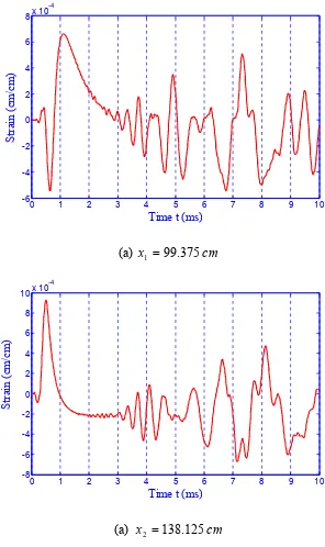
cm

x₁ =99.375 and x₂ =138.125cm, which are shown in Fig. 3.4. As mentioned

before, dispersion of the wave is relatively severe and low frequency components propagate at the relatively low velocities in this case. Although the intensive part is the waveform without deflection from the ends, for clarity, the duration is taken as long as 10

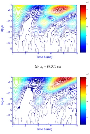
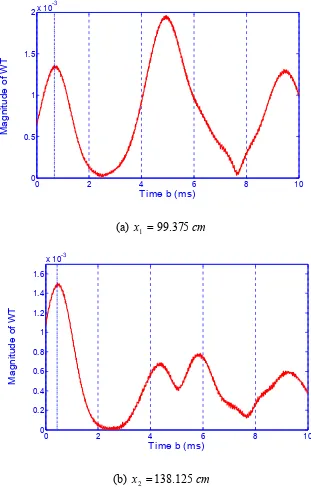
ms so that the low frequency components can be included. Fig. 3.6 shows the contour

plot of the time-frequency distribution of the WT of two signals. The scale a shown in

the Fig. 3.4 can be converted to the corresponding frequency as

a

f = 1 (3.4.3)