INVESTIGATION
Complete Numerical Solution of the Diffusion
Equation of Random Genetic Drift
Lei Zhao,* Xingye Yue,†and David Waxman*,1 *Centre for Computational Systems Biology, Fudan University, Shanghai 20433, People’s Republic of China and†Department of Mathematics, Suzhou University, Suzhou 215006, People’s Republic of China
ABSTRACT A numerical method is presented to solve the diffusion equation for the random genetic drift that occurs at a single unlinked locus with two alleles. The method was designed to conserve probability, and the resulting numerical solution represents a probability distribution whose total probability is unity. We describe solutions of the diffusion equation whose total probability is unity ascomplete. Thus the numerical method introduced in this work produces complete solutions, and such solutions have the property that whenever fixation and loss can occur, they are automatically included within the solution. This feature demonstrates that the diffusion approximation can describe not only internal allele frequencies, but also the boundary frequencies zero and one. The numerical approach presented here constitutes a single inclusive framework from which to perform calculations for random genetic drift. It has a straightforward implementation, allowing it to be applied to a wide variety of problems, including those with time-dependent parameters, such as changing population sizes. As tests and illustrations of the numerical method, it is used to determine: (i) the probability density and time-dependent probability offixation for a neutral locus in a population of constant size; (ii) the probability offixation in the presence of selection; and (iii) the probability offixation in the presence of selection and demographic change, the latter in the form of a changing population size.
R
ANDOM genetic drift occurs when genes of a given type are transmitted to the next generation with random variation in their number. It occurs when the relevant num-ber of genes isfinite and not effectively infinite. The process of random genetic drift plays a fundamental role in molec-ular evolution and the behavior of genes infinite populations (Crow and Kimura 1970; Kimura 1983). Beyond this, some of the ideas and techniques used in random genetic drift have a wider use, for example, with applications to cancer (Zhuet al.2011; Traulsenet al.2013) and range expansion (Slatkin and Excoffier 2012).To set the stage for the present work, consider a single locus with genetic variation due to the segregation of more than one allele in the population. The population size is assumed finite, so random genetic drift generally occurs, and the number of copies of a particular allele at the locus changes randomly over time. The genetic composition of the population exhibits a particular sort of random walk and
a distribution describing such walks can be analyzed under an approximation where it obeys a diffusion equation. This treatment of random genetic drift is naturally known as the diffusion approximation and was introduced into population genetics by Fisher (1922) and Wright (1945) and substantially extended and developed by Kimura (1955a); the diffusion approximation continues to be developed and applied in a variety of situations (Ewens 2004).
The diffusion approximation is often applied to the Wright–Fisher model (Fisher 1930; Wright 1931), where both time and the possible frequencies of an allele take discrete values. Such a“discrete”model has a mathematical description involving matrices and vectors, and numerical results for simple situations can be directly obtained on the computer. A comparison of Wright–Fisher and diffusion results suggest that the diffusion approximation is usually very accurate. It is known to work well when the number of individuals is not large (10) when selection is not strong (Ewens 1963). Generally, however, the accuracy of the dif-fusion approximation depends on the population size and the strength of selection, as discussed in the book by Ewens (2004). The book by Gale (1990) also discusses limitations of this approximation.
Copyright © 2013 by the Genetics Society of America doi: 10.1534/genetics.113.152017
Manuscript received April 5, 2013; accepted for publication June 2, 2013 1Corresponding author: Centre for Computational Systems Biology, Fudan University,
For an appreciable population size, or in complex situations, such as a changing population size, the diffusion equation, should, in principle at least, come into its own right, and be preferable to the Wright–Fisher model. For example, if the population size changes over time, the Wright–Fisher model becomes complicated by its matrix of transition probabilities changing size over time (the size of the matrix depends on the size of the population). By contrast, in a diffusion analysis only a parameter in the diffusion equation changes over time; the form and description of the diffusion equation are not depen-dent on the value of this parameter. The diffusion approxima-tion has some other advantages.
In some cases the diffusion equation can yield explicit mathematical results; however, beyond this, the diffusion equation has the property of accessibly displaying key parameters of a problem (e.g., the effective population size, the strength of selection, mutation rates,...). A consequence is that the diffusion equation can be subject to mathematical transformations that expose the dependence of a solution on important combinations of these parameters. As an example, consider an unlinked locus with two alleles, which is subject to semidominant selection of strengths(with |s|1) and two-way mutation at rateu. It can be shown that the diffu-sion equation leads, after the rescaling of time by the effec-tive population size,Ne, to an equation that depends on the
composite parameters Nes and Neu, rather than separately
depending onNe,s, andu. Thus one conclusion that may be
immediately drawn, without actually solving the diffusion equation, is that the equilibrium distribution of the allele frequency (which does not involve time) depends only on the composite parametersNesandNeu. Hence a locus with
Ne= 100,s= 1022, andu= 1025and another withNe=
1000,s= 1023, andu= 1026will both, under the diffusion
approximation, be described by the same equilibrium distri-bution of the allele frequency, because both haveNes= 1 and
Neu = 1023. More generally, the ability to mathematically
transform the diffusion equation can lead to understanding of the properties of whole sets of solutions (in the above example, all equilibrium solutions with given values of Nes
andNeu) along with other properties (Waxman 2011b).
While knowledge of the distribution of the allele frequency is important and useful, exact time-dependent solutions of the diffusion equation for two alleles are known in only a relatively small number of cases, such as under neutrality, where Kimura (1955b) obtained the part of the solution associated with segregating alleles, while McKane and Waxman (2007) derived the corresponding solution that also includes fixation and loss. Other known solutions incorporate migration or mutation (Crow and Kimura 1956, 1970). To analyze interesting new situations, which are con-stantly arising (for example, see Wylieet al.2009) requires additional solutions of the diffusion equation and a numeri-cal approach appears to be the simplest way forward.
In this work we present a scheme for numerically solving the diffusion equation. This approach can benefit from the advantages, alluded to above, of the diffusion approximation.
In our view, the numerical scheme provides a viable way of investigating problems in random genetic drift; as we show, it can be simply applied to complex situations.
The numerical scheme is designed to lead to a normalized probability distribution in which the total probability sums (or integrates) to unity at all times. We describe solutions of the diffusion equation, whose total probability is unity, as complete. Thus the numerical method presented here pro-duces complete solutions. Before we say more about the nu-merical scheme, let us discuss features of complete solutions. A key feature of acompletesolution of the diffusion equa-tion is that all possible outcomes are included, by virtue of the total probability of the distribution summing to unity. Thus iffixation and loss are possible, then populations with
fixed, lost, and segregating alleles are all, necessarily, in-cluded in a complete solution.
There are fundamental reasons for wishing to consider complete solutions of the diffusion equation, apart from the fact that they conserve probability and constitute a complete description. Such solutions have properties that are in extremely close correspondence with those of the model underlying the diffusion approximation—the Wright–Fisher model. As an example, in a Wright–Fisher model for a neu-tral locus, the expected value of the (relative) frequency of an allele, at any time, coincides with the initial value of its frequency (which is assumed known precisely). Under a dif-fusion analysis, exactly the same property of the expected value of the allele frequency holds only when a complete solution of the diffusion equation is used to carry out the average; using a solution that covers only populations with segregating alleles will not lead to the expected frequency of an allele coinciding with its initial value. Such an expecta-tion requires an average that is taken not only over popula-tions in which alleles are segregating, but also must include populations in which alleles havefixed or been lost.
When the phenomena of loss andfixation can occur, math-ematical treatments of the diffusion equation lead to complete solutions that have been found to contain singularities—sharp spikes (i.e., Dirac delta functions) at the frequencies zero and one (McKane and Waxman 2007; Chalub and Souza 2009; Waxman 2011a). The spikes in the solution are distributions with zero width butfinite area. They represent probability densities of lost andfixed alleles. The spikes are the way the probabilities of the terminal frequencies of the Wright–Fisher model arise within the diffusion approximation (Waxman 2011a).
The numerical approach presented here technically in-volves solving the forward diffusion equation (Otto and Day 2007) for the probability distribution of the frequency of an allele. In contrast to the previous approaches, we look for a complete solution that conserves probability. However, at
first sight it is unclear how to determine such a numerical solution iffixation or loss are possible, since singular spikes are present in the exact solution, and these appear to be numerically intractable, given their zero width. Further-more, even solutions that do not possess singular spikes may have very sharp features at the boundary frequencies of zero and one due,e.g., to low mutation rates.
The numerical method of this work evades problems by not directly dealing with actual values of a solution, which would diverge at any spikes present. Rather, the method deals with frequency averages. A solution of the diffusion equation is discretized into frequency bins of finite width, and the value of this solution across a bin is a constant that represents an average of the exact solution across the bin. Since this average value, when multiplied by the bin width, represents a probability, it has afinite value, irrespective of any singular behavior of the underlying exact solution. The resulting discretized/averaged solution is treated by a so-called“finite volume”numerical scheme, which is of a type used forfluids. Such a scheme conserves the total probabil-ity, in the same way that the volume of a fluid of constant density is conserved. Given that this numerical method is based on a discretization, it cannot explicitly show the pres-ence of singular, zero width spikes within the solution. How-ever, in the Results we show that it is possible to clearly demonstrate the presence and contribution of such singular features within a solution.
Overall, a complete numerical solution of the diffusion equation, as presented in this work, allows a wide range of problems to be addressed, including time-dependent selec-tion and changing populaselec-tion sizes, within a single inclusive and mathematically consistent framework.
Diffusion Equation
To proceed, let us consider the standard case of a single un-linked locus in a randomly mating diploid sexual population. The locus has two alleles, denotedAandB, and generations are taken to be non overlapping. The processes occurring in one generation are given in the following lifecycle:
Adults ðgeneration tÞ
Y reproduction; followed by the death of all adults
Zygotes
Y selection
Juveniles
Y thinning ðpopulation number regulationÞ
Adults ðgeneration tþ1Þ
Based on the assumption that each adult contributes to a very large number of zygotes, the processes of both re-production and selection are treated as being deterministic
in character, meaning that there are negligible deviations from expected behaviors.
The individuals who survive selection (juveniles) are subject to a nonselective process of ecological thinning. In this process, N individuals are randomly picked, without regard to genotype, from an assumed much larger number of individuals, to become theNadults of the next genera-tion. All randomness in the lifecycle, which directly arises from random genetic drift, occurs during the thinning stage of the lifecycle.
The proportion of all genes at the locus, in adults, that are theAallele is the relative frequency of this allele. Hence-forth we refer to the relative frequency as just the frequency. The process of thinning generally results in the frequency varying randomly from generation to generation and we write its value at time tasX(t). This random variable gen-erally takes different values in different copies of a popula-tion. Statistics of the frequency are described by a Wright– Fisher model (Fisher 1930; Wright 1931) and are expressed in terms of a discrete probability distribution, which can be thought of as describing the behavior ofX(t) in a very large number of replicate populations. Under a diffusion approx-imation, however, both time and the frequency are treated as continuous quantities, and the statistical description of the allele frequency is given in terms of a probabilitydensity (but following common usage we use the phrases probabil-ity densprobabil-ity and probabilprobabil-ity distribution interchangeably in what follows). The probability density of the frequency of theAallele at timet, when the value of the frequency isx, is written asf(x,t), and this obeys the diffusion equation
2@@
tfðx;tÞ ¼2 1 4NeðtÞ
@2
@x2½xð12xÞfðx;tÞ
þ@@
x½Mðx;tÞfðx;tÞ (1)
(Kimura 1955a, 1964). In this equation, the function M(x, t), which is typically a polynomial in x, incorporates the forces of migration, mutation, and selection, which are act-ing at time t(and in an infinite population M(x,t) would drive changes in the allele frequency), whileNe(t) denotes
the variance effective population size at timet.
Note that theoretically, the variance effective size,Ne(t),
is determined from processes that occur over a single gen-eration (Ewens 2004). We use Ne(t) to refer only to this
quantity, and in particular, we do not make use of averages of the effective population size, such as the harmonic mean, which summarize the values taken by the effective popula-tion size over multiple generapopula-tions.
When mutation may be neglected, but AA, AB, and BB genotype individuals have relativefitnesses of 1 +s, 1 +hs, and 1, respectively, assuming |s| and |sh| are small (1), we haveM(x) =sx(12x)[x+h(122x)] (Ewens 2004). A special case of this scheme of selection, termed semidomi-nantselection, occurs whenh=1
2. Furthermore,
selection, in which the relative fitnesses of the three geno-types are (1 +s)2, 1 +s, and 1, respectively, in which case
M(x) =sx(12x).
Numerical Scheme
Equation 1 can be written in the form
@fðx;tÞ @t þ
@jðx;tÞ
@x ¼0; (2)
where
jðx;tÞ ¼ 2 1 4NeðtÞ
@
@x½xð12xÞfðx;tÞ þMðx;tÞfðx;tÞ (3)
is the probability current density. The quantityj(x,t) repre-sents aflow of probability and Equation 2 ensures that prob-ability is rather like afluid, in the sense that all changes in the probability contained in a region ofxoccur only because of aflow of probability, via the probability current, in or out of that region.
In the diffusion equation, conservation of total proba-bility follows from the appropriate specification of the probability current at the terminal allele frequencies x= 0 andx= 1. Following McKane and Waxman (2007), we impose conditions that ensure that there is no flow of probability beyond the terminal allele frequencies, by re-quiring the probability current density to vanish at both x= 0 andx= 1. These conditions, combined with Equa-tion 2 ensure that the total probability, R01fðx;tÞdx, has a constant value for all times. A consequence of this is that fixation and loss are naturally included within the solution (McKane and Waxman 2007; Waxman 2011a). In this work, we present a numerical scheme for the so-lution of the diffusion equation where the total probabil-ity is conserved at all times. The scheme is similar to the sort used onfluids of constant density, where conservation of the total quantity of the fluid (analogous to the total probability) is maintained at all times.
Implementation of the numerical scheme
We first give a direct statement of the numerical scheme. Detailed aspects of the scheme are discussed immediately afterward.
The values of the frequency,x, are discretized into a grid with spacinge. The grid points lie atxi=i·e,wherei= 0, 1, 2,. . .,K, and we takee= 1/K; hence the values of thexi range from 0 to 1. Times are also discretized, with a step size oft and grid points attn=n·t,wheren= 0, 1, 2,. . ..
The numerical scheme determines an approximate, dis-cretized form of the allele frequency’s probability density, f(x, t). In particular, the scheme determines quantities we write asfn
i, with eachfinrepresenting theapproximatevalue of f(x, tn), when averaged over a range of x near xi (see Interpretation of the numerical scheme for a more detailed explanation of the fn
i). We call the K+ 1 values of f n
0,f1n, . . .,fn
K therepresentation of the distribution f(x,tn).
Given theK+ 1 values of the representation off(x,tn), the numerical scheme determines the K+ 1 values of the representation off(x,tn+1), namelyf0nþ1,f
nþ1 1 ,. . .,f
nþ1
K . The numerical scheme can be compactly written as the matrix equation
fðnþ1Þ¼
h
1þaRðnþ1Þ
i21h
12aRðnÞ
i
fðnÞ: (4)
In this equation:
1. f(n) denotes aK+ 1 componentcolumnvector for time
steptn. The elements off(n)arefinwithi= 0, 1, 2,. . .,K and sof(n) contains the representation off(x,t
n). 2. ais a constant, arising from the discretization ofxandt,
and takes the form
a¼2et2: (5)
3. R(n)is a matrix of size (K + 1)·(K+ 1) that generally
depends on the time,tn. To defineR(n)we introduce
Uni ¼2
xið12xiÞ
4NeðtnÞ þ
eMðxi;tnÞ
2 ; V
n i ¼
xið12xiÞ
4NeðtnÞ þ
eMðxi;tnÞ
2 :
(6)
Then elements ofR(n)are written asRðnÞ
i;j wherei,j= 0, 1, 2, . . .,K. The only nonzeroRði;njÞ havei=j andi=j 61; hence R(n) has the form of a tridiagonal matrix. For
exam-ple, for K= 4 the nonzero elements are
RðnÞ¼
0 B B B B @
n n n n n
n n n n n n
n n 1 C C C C A:
Generally, the nonzero elements ofR(n)are
Leading upper diagonal: R0ðn;1Þ¼2Un
1
Rði;niþÞ1¼Un
iþ1 for 1#i#K21
Main diagonal: Rð0n;0Þ¼2Vn
0
Rði;niÞ¼Vn i 2Uin
RðKn;ÞK¼ 22Un K
for 1#i#K21
Leading lower diagonal: Rið;ni2Þ1¼2Vi2n1
RðKn;ÞK21¼22Vn K21:
for 1#i#K21
UsingR(n)within Equation 4 completes the specification of
Equation 4 generally relies on inverting the matrix 1+ aR(n). When the condition |s| #K/[2N
e(tn)] applies, the matrix is invertible for all values of the constantaof Equa-tion 5. We have used values ofaas large asa= 1000 with good results. Full details of the derivation of the numerical scheme are given inAppendix A.
Interpretation of the numerical scheme
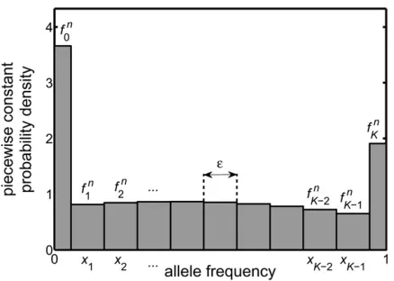
If the probability densityf(x,t) were a smooth function of the frequency,x, then its behavior at a given time would be reasonably summarized by the approximate values it takes at the discrete pointsxi. Potentially, however, we have a dis-tribution that contains spikes (Dirac delta functions), i.e., singular features that change arbitrarily rapidly. For this rea-son, wefirst replacef(x,t) with a probability density that is piecewise constant. This is obtained by splitting the range of possible frequencies, 0#x#1, into a set of intervals and replacingf(x,t) in each interval by a constant that equals its average value over the interval. The numerical scheme pre-sented here determines anapproximationof these average values, at the discrete timestn. The quantityfinthus denotes theapproximatevalue off(x,tn),afterit has been averaged over a range ofxnearxi. To be specific:
i. The quantityfn
0 is the approximate value off(x,tn), when averaged over x in the range x0 [ 0 to x1/2, i.e., over
a range of width e/2. This is equivalent to saying Rx1=2
0 fðx;tnÞdx ðe=2Þf0n.
ii. For i= 1, 2, . . ., K21, the quantity fn
i represents the approximate value of f(x,tn), when averaged over xin the rangexi21/2to xi+1/2, i.e., over a range of width e.
This is equivalent to sayingRxiþ1=2
xi21=2 fðx;tnÞdxefin. iii. The quantityfn
K represents the approximate value off(x, tn), when averaged overxin the rangexK21/2toxK[1, i.e., over a range of width e/2. This is equivalent to sayingRx1
K21=2fðx;tnÞdx ðe=2Þf
n K.
Figure 1 illustrates the piecewise constant probability den-sity that is determined by thefn
i.
We can use the numerical approximation of the proba-bility density, f(x,t), to calculate the average of a quantity such asG(X(t)), whereX(t) is the random value of the allele frequency at timet. We work under the assumption that the functionG(x) is continuous. The expected or average value of G(X(t)) is written as E[G(X(t)], and under the diffusion approximation E½GðXðtÞ ¼R01GðxÞfðx;tÞdx. Using the nu-merical approximation we take
E½GðXðtnÞe
2Gð0Þf
n
0 þe X
K21
i¼1
GðxiÞfinþ
e 2Gð1Þf
n
K: (7)
Note that conservation of probability means that the total probability has a value of unity ðR01fðx;tÞdx¼1Þ, indepen-dent of the value of time,t. This result, in conjunction with Equation 7, suggests that
CðtnÞ[
defe
2f
n
0þe X
K21
i¼1 finþe
2f
n K;
which is the numerical analog of R01fðx;tnÞdx, takes the value of unity, independent of the value of the time tn. In Appendix Bwe show that the numerical scheme given above yieldsC(tn) = 1 for alltn.
Results
Determining the solution of the diffusion equation
We first apply the numerical scheme of Equation 4 to the fundamental problem of determining the solution of the diffusion equation at timetand frequencyx, given an initial distribution at timet= 0. This solution, which is a probabil-ity densprobabil-ity, can be used to determine the expected value of any statistic that depends on the allele frequency at timet. For an initial distribution that is very narrowly peaked around a single frequency, the behavior of the numerically calculated distribution is illustrated in Figure 2 indicates spike-like parts of the solution developing over time.
Evidence of spikes in the solution
In the analysis of McKane and Waxman (2007) and Waxman (2011a), it was indicated that when the total probability is Figure 1 The numerical approximation replaces the exact probability
density of the diffusion equation at time tn, namely f(x, tn), by the
approximate piecewise constant probability density shown in thefi g-ure. This approximate distribution is determined by discretizing, aver-aging, and approximating the equation obeyed by f(x, t) and then iterating the resulting equation. It leads to the quantitiesfn
i, each of
which is a numerical approximation of the average value of f(x,tn),
with the average taken over a range ofxnear the grid pointxi(see
conserved, exact solutions of the diffusion equation describe populations where alleles are fixed, lost, or are segregating and that these solutions generally contain spikes. However, the numerical approach presented above is obtained by dis-cretizing the frequency intofinite-width bins. Thus it is clear that no spike, which has zero width, can bedirectlyseen un-der the numerical approach. To investigate the content of the numerical approach, let us consider the last two bins on the right in Figure 1. These are binK21 and binKand the corresponding values of the distribution are fn
K21 and fKn. These bins cover the frequency ranges xK23/2 to xK21/2
and xK21/2to xKand hence have widths of eand e/2, re-spectively. Let us write the probability of finding the fre-quency in these intervals, as calculated from the numerical scheme, aspK21(e) andpK(e) respectively, thenpK21ðeÞ ¼efKn21
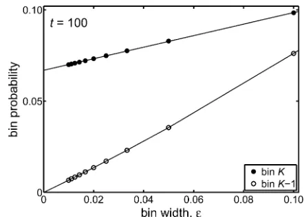
andpKðeÞ ¼ ðe=2ÞfKn. The behavior we observe, on progres-sively reducingeand hence the width of both bins, is shown in Figure 3.
For the parameters adopted for Figure 3, the behavior of the probabilities exhibited are very well described by
pK21ðeÞ ¼a·eþb·e2
pKðeÞ ¼cþd·e; (8)
wherea,b,c, anddare independent ofebut depend on the time at which the distribution is evaluated. The significant fact is that ase/0 the probabilitypK21(e) associated with
bin K 21 tends toward a very small number that cannot be meaningfully distinguished from zero but the probability of the end bin,pK(e), tends to a constant (namelyc). Since pK21(e) andpK(e) are numerical estimates of
RxK21=2
xK23=2 fðx;tnÞdx
andRx1
K21=2fðx;tnÞdx, the behaviors exhibited in Figure 3 and
Equation 8, ase/0, are fully consistent with the theoret-ical prediction that the distributionf(x,t) contains a spike (a Dirac delta function) whose weight is located at x= 1; so pK(e) obtains the entire contribution from the spike butpK21 (e)obtains no contribution.
The quantityc=c(tn), which is thelimiting valueofpK(e) aseapproaches 0, is a numerical estimate of the probability that the frequency x= 1 has been reached by timetn. It is thus an estimate of the probability offixation by timetnand Figure 2 Solutions of the diffusion equation at different times that
were obtained using the numerical method of this work. The figure covers the neutral case, with no selection, mutation, or migration, and the effective population size adopted wasNe= 100. When implement-ing the numerical method, we arbitrarily chose a time step oft= 0.1 and a frequency step ofe= 0.02 (i.e.,K= 50). The initial time was taken ast= 0 and the initial distribution had only a single of thef0 i
being nonzero, corresponding to an initial frequency ofy= 0.3. Such an initial distribution is indistinguishable from the initial frequency being uniformly distributed over an interval of widthethat is centered aty= 0.3. We note that during the time interval used in thefigure (50 generations), spike-like parts of the distribution appear at the fre-quency 0. As shown in the text, these are fully consistent with the presence of a spike (Dirac delta function) in the full diffusion solution atx= 0, representing populations that have lost theAallele. Evaluating the solution for a longer time (results not shown) also leads to a spike-like part developing at x = 1, signaling populations wherefixation occurs. Exact properties of the diffusion solution are that: (i) the dis-tribution remains normalized for all times and (ii) the expected value of the frequency at timet, given an initial distribution that is symmetric about the frequencyy, obeysE[X(t)] =y(this result is particular to the neutral case). Wefind that properties i and ii are both obeyed by the numerical solution to an accuracy of approximately one part in 1014, which is close to the precision of the software used in the calculations (MATLAB).
Figure 3 We show how the probabilities associated with the numer-ically determined probability density change when the spacing of discrete frequencies,e, is reduced. We considered the piecewise con-stant probability distribution at a discrete time corresponding tot= 100 generations. To make the numerical calculation of all probabil-ities as comparable as possible, we set the ratio aof Equation 5, which characterizes the numerical scheme, to have the value a = 500. We then determined the time step, for a given value ofe, from t= 2e2aand the time index fromn= 100/t. Thus different points of thefigure are associated with differenteand hence differenttandn, but the values oftandaare heldfixed. The probabilities associated with the last two bins on the right in Figure 1, namely binK21 and binK, arepK21ðeÞ ¼efKn21andpKðeÞ ¼ ðe=2ÞfKn, respectively. We
ob-serve in Figure 3 that wheneapproaches 0, the probabilitypK21(e),
associated with binK21, converges to a small number that, within numerical error, may be taken as zero. However the probabilitypK(e),
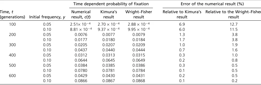
can also be described as the time-dependent probability of fixation. In addition to this numerical result, we have Kimura’s result for the time-dependent probability offixation, which was derived from the diffusion equation for the neutral case (Kimura 1955b). In Table 1 we give results of both meth-ods of calculation of the time-dependent probability offixation andfind small percentage differences in a variety of differ-ent cases.
Inclusion of selection
Table 1 and Figures 2 and 3 cover the random genetic drift of alleles at a neutral locus. We can, additionally, test the accuracy with which the numerical method can deal with selection. For genic selection (whereAA,AB, andBB geno-type individuals have relative fitnesses of (1 +s)2, 1 + s,
and 1, respectively) the probability ofultimatefixation (t/
N) from an initial frequency ofyis given, under the diffu-sion approximation, by
PfixðyÞ ¼
12e24Nesy
12e24Nes (9)
(Kimura 1962). In Table 2 we compare the result of the numerical method with Equation 9. Very reasonable agree-ment is seen in Table 2 between the numerical results and the exact diffusion results.
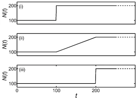
Demographic change
As a final test of the numerical method, let us investigate some nontrivial cases with no known explicit results. We consider the probability of ultimate fixation, under genic selection of strength s, when the population size changes over time. For the purposes of this test, we assume that the effective population size coincides with the census size and consider the population-size behaviors given in Figure 4.
WithPfix(y) the probability of ultimate fixation from an
initial frequency of y at time 0, we use three different approaches to estimate this quantity:
i. A direct approach: Use the numerical scheme to deter-mine the probability density of the frequency at very long times. The distribution then reduces to only the terminal bins having nonzero probability. The probability associ-ated with binK, namely the large nlimit of ðe=2Þfn
K, can be used to estimate of the probability offixation. ii. A less direct, but efficient approach: Use a special case of
a result of Waxman (2011b), which is based on the dif-fusion approximation. When the population size has ar-bitrary changes from time 0 to time T, but remains constant after timeT, the probability offixation is
PfixðyÞ ¼
Z 1
0
12e24NðTÞsx
12e24NðTÞsfðx;T;yÞdx: (10)
Here we have extended the notation slightly and usedf(x,T; y) to denote the complete probability density of the fre-quency at time T, given that the initial frequency at time 0 is y. Note that f(x, T; y) is the probability density after the population size has stopped changing. Equation 10 has the advantage that it requires only the distribution at timeT. Thus for populations that change according to Figure 4, it requires only the distribution of the frequency forfinite val-ues of T (namely 100 and 200 generations) and not for longer times. This considerably reduces the amount of com-putation compared with the direct method of approach i.
Since Equation 10 follows from an average of Kimura’s result for the fixation probability, Equation 9, we refer to Equation 10 as the “averaged Kimura result.” InAppendix Table 1 Results for the time-dependent probability offixation at a neutral locus when the effective population size isNe= 100
Time,t
(generations) Initial frequency,y
Time dependent probability offixation Error of the numerical result (%)
Numerical result,c(t)
Kimura’s result
Wright–Fisher result
Relative to Kimura’s result
Relative to the Wright–Fisher result
100 0.05 2.51·1024 2.70·1024 2.88·1024 6.9 12.7
0.10 8.81·1024 9.37·1024 9.95·1024 6.0 11.5
200 0.05 0.0076 0.0077 0.0079 1.3 3.8
0.10 0.0177 0.0180 0.0184 1.7 3.8
300 0.05 0.0205 0.0207 0.0209 1.0 1.9
0.10 0.0437 0.0440 0.0444 0.7 1.6
400 0.05 0.0312 0.0313 0.0315 0.3 1.0
0.10 0.0644 0.0645 0.0649 0.2 0.8
500 0.05 0.0384 0.0385 0.0386 0.3 0.5
0.10 0.0780 0.0781 0.0784 0.1 0.5
600 0.05 0.0429 0.0430 0.0431 0.2 0.5
0.10 0.0866 0.0867 0.0868 0.1 0.2
This table gives results for the time-dependent probability offixation at a neutral locus when the effective population size isNe¼100. It covers different values of the initial frequency,y, and different values of the time,t. The results were obtained from the numerical scheme of this work, Kimura’s expression for the time-dependent probability of fixation, which took the form of an infinite sum (Kimura 1955b), and the Wright–Fisher model. For the numerical calculations, wefixed the ratioa, Equation 5, at the value
C we give further details of how thefixation probability is determined by this method.
iii. Simulation: As the third andfinal method of estimating thefixation probability, we simulated a large number of replicate populations, which all started with an Aallele frequency of y. All simulations were made within the framework of a Wright–Fisher model (Fisher 1930; Wright 1931); for more details see the caption of Table 3. The simulations were continued until all populations eitherfixed or lost theAallele. An estimate ofPfix(y) was
then obtained from the proportion of all of the replicate populations where theAallele hadfixed.
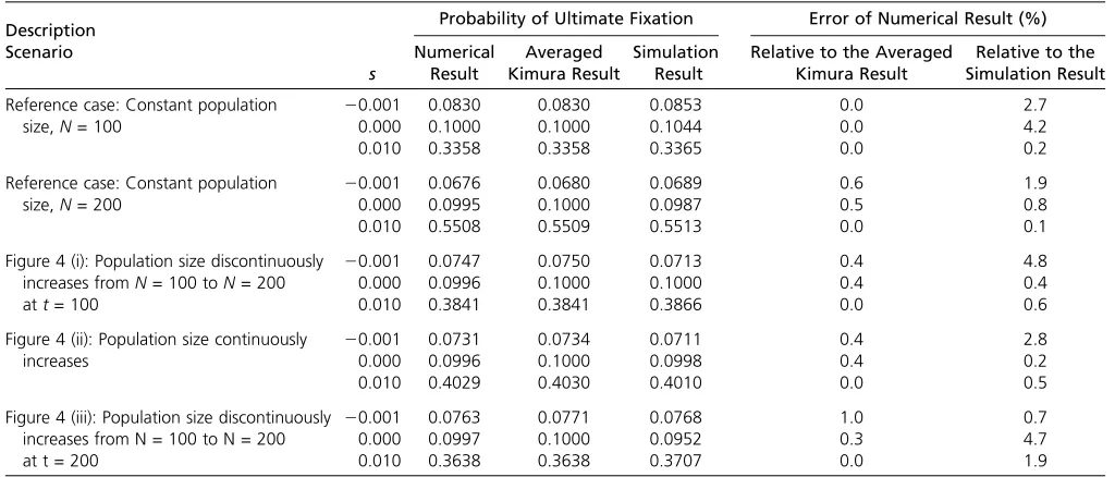
The results obtained from approaches i, ii, and iii are summarized in Table 3. The overall conclusion is that all three methods of calculation agree well with one another.
Discussion
In this work we have presented a method of numerically solving the diffusion equation for the random genetic drift of the frequency of an allele. We imposed “zero current” boundary conditions at the frequenciesx= 0 andx= 1 to ensure that the total probability associated with the distri-bution remains independent of time. Such an approach au-tomatically leads to the incorporation of fixation and loss into the distribution of allele frequencies—when it is possi-ble for these to occur. In situations where fixation and loss cannot occur, such as when there is two-way mutation, the zero current boundary conditions lead to solutions of the diffusion equation that, theoretically, do not possess singular spikes. In this case, we find that under the numerical scheme, the probability associated with any bin decreases as the splitting of discrete frequencies,e, decreases (results not shown), giving similar behavior to that of binK21 in Figure 3. This behavior is consistent with there being no spike present in the solution. It thus appears that zero cur-rent boundary conditions appear to capture all aspects of the genetic drift process.
The numerical scheme introduced in this work was applied to a number of different problems, as summarized in Tables 1, 2, and 3, including the time development prob-ability of fixation and the probability of ultimate fixation when the population size changes over time. For relatively modest population sizes we found very reasonable results. For example, in Table 3, differences between simulation results and the numerical results were of the order of a few percent. These results give us good confidence in the validity and robustness of the numerical scheme.
The mathematical aspects of this problem involve singu-lar spikes (Dirac delta functions) in exact solutions of the diffusion equation and direct manifestations of these fea-tures are seen in the numerical solutions. These ultimately result from the boundary condition imposed on the solu-tions, namely there being zero probability current density at the frequenciesx= 0 andx= 1. InAppendix Dwe discuss the possibility of other boundary conditions. It turns out that “natural” boundary conditions, which do not need to be externally imposed and, indeed, follow directly from the
Figure 4 Different scenarios of population size change that are used in a test of the numerical method of this work. The corresponding results for the probability of ultimatefixation are given in Table 3.
Table 2 Results for the probability of ultimate fixation at a locus subject to genic selection when the effective population size isNe= 100
4Nes Initial frequency, y
Probability of ultimatefixation
Relative error (%) Numerical result,c(N) Kimura’s result
21 0.05 0.0297 0.0298 0.3
0.10 0.0608 0.0612 0.7
0 0.05 0.0496 0.0500 0.8
0.10 0.0993 0.1000 0.7
10 0.05 0.3934 0.3935 ,0.1
0.10 0.6321 0.6321 ,0.1
diffusion equation, are another possibility, and these have been implicitly adopted in the past (Kimura 1955b; Barakat and Wagener 1978; Wang and Rannala 2004). However, these boundary conditions do not result in conservation of probability or the presence of singular spikes in solutions.
The numerical approach has another aspect that we have not pursued: it gives an expression for the probabil-ity current densprobabil-ity (see Equation A.11). Thus, unlike the Wright–Fisher model, it is possible to determine the numer-ical value of the probability current density at any time and at any frequency. This might have some interest in its own right.
The diffusion equation for random genetic drift has been in existence for a considerable period of time. The present work provides, we believe, the first method for directly
finding a complete numerical solution (i.e., a distribution with a total probability of unity). The delay infinding such a solution may be attributable to the diffusion equation hav-ing shav-ingular features, i.e., zero width spikes, which lie be-yond the features normally encountered in the literature. We have illustrated the accuracy of the numerical solution with a number of examples (see Tables 1, 2, and 3). The numerical method presented here can be easily and rapidly implemented; we believe it should have applications in the analysis and exploration of random genetic drift in genetics and related subjects, wherever the diffusion equation occurs.
Acknowledgments
It is a pleasure to thank Jianfeng Feng, Martin Lascoux, Andy Overall, Joel Peck, and Chenyang Tao for helpful discussions. We thank the handling editor Wolfgang Stephan and two anonymous reviewers for comments and sugges-tions, which have improved this work. X.Y. was supported in part by the National Science Foundation of China under grant no. 11271281.
Literature Cited
Barakat, R., and D. Wagener, 1978 Solutions of the forward dia-llelic diffusion equation in population genetics. Math. Biosci. 41: 65–79.
Chalub, F. A. C. C., and M. O. Souza, 2009 A non-standard evo-lution problem arising in population genetics. Commun. Math. Sci. 7: 489–502.
Crow, J. F., and M. Kimura, 1956 Some genetic problems in nat-ural populations. Proc. Third Berkeley Symp. Math. Stat. and Prob. 4: 1–22.
Crow, J. F., and M. Kimura, 1970 An Introduction to Population Genetics Theory. Harper & Row, New York.
Demmel, J. W., 1997 Applied Numerical Linear Algebra. Society for Industrial and Applied Mathematics, Philadelphia.
Engelmann, B., F. Koster, and D. Oeltz, 2011 Calibration of the Heston Stochastic Local Volatility Model: A Finite Volume Scheme. Available at: http://ssrn.com/abstract=1823769 or http://dx.doi.org/10.2139/ssrn.1823769.
Table 3 Comparison of the effects of different scenarios of demographic change on the probability of ultimatefixation when the initial frequency isy= 0.1
Description Probability of Ultimate Fixation Error of Numerical Result (%)
Scenario
s NumericalResult
Averaged Kimura Result
Simulation Result
Relative to the Averaged Kimura Result
Relative to the Simulation Result
Reference case: Constant population size,N= 100
20.001 0.0830 0.0830 0.0853 0.0 2.7
0.000 0.1000 0.1000 0.1044 0.0 4.2
0.010 0.3358 0.3358 0.3365 0.0 0.2
Reference case: Constant population size,N= 200
20.001 0.0676 0.0680 0.0689 0.6 1.9
0.000 0.0995 0.1000 0.0987 0.5 0.8
0.010 0.5508 0.5509 0.5513 0.0 0.1
Figure 4 (i): Population size discontinuously increases fromN= 100 toN= 200 att= 100
20.001 0.0747 0.0750 0.0713 0.4 4.8
0.000 0.0996 0.1000 0.1000 0.4 0.4
0.010 0.3841 0.3841 0.3866 0.0 0.6
Figure 4 (ii): Population size continuously increases
20.001 0.0731 0.0734 0.0711 0.4 2.8
0.000 0.0996 0.1000 0.0998 0.4 0.2
0.010 0.4029 0.4030 0.4010 0.0 0.5
Figure 4 (iii): Population size discontinuously increases from N = 100 to N = 200 at t = 200
20.001 0.0763 0.0771 0.0768 1.0 0.7
0.000 0.0997 0.1000 0.0952 0.3 4.7
0.010 0.3638 0.3638 0.3707 0.0 1.9
Ewens, W. J., 1963 Numerical results and diffusion approxima-tions in a genetic process. Biometrika 50: 241–249.
Ewens, W. J., 2004 Mathematical Population Genetics. I. Theoret-ical Introduction. Springer-Verlag, New York.
Fisher, R. A., 1922 On the dominance ratio. Proc. R. Soc. Edinb. 42: 321–341.
Fisher, R. A., 1930 The Genetical Theory of Natural Selection. Clar-endon Press, Oxford.
Gale, J. S., 1990 Theoretical Population Genetics. Unwin Hyman, London.
Kimura, M., 1955a Stochastic processes and distribution of gene frequencies under natural selection. Cold Spring Harb. Symp. Quant. Biol. 20: 33–53.
Kimura, M., 1955b Solution of a process of random genetic drift with a continuous model. Proc. Natl. Acad. Sci. USA 41: 141– 150.
Kimura, M., 1962 On the probability offixation of mutant genes in a population. Genetics 47: 713–719.
Kimura, M., 1964 Diffusion models in population genetics. J. Appl. Probab. 1: 177–232.
Kimura, M., 1983 The Neutral Theory of Molecular Evolution. Cam-bridge University Press, CamCam-bridge, UK.
McKane, A. J., and D. Waxman, 2007 Singular solutions of the diffusion equation of population genetics. J. Theor. Biol. 247: 849–858.
Morton, K. W., and D. F. Mayers, 2005 Numerical Solution of Partial Differential Equations. Cambridge University Press, Cam-bridge, UK.
Oleinik, Q. A., and E. V. Radkevic, 1973 Second Order Equations with Non-negative Characteristic Form. American Mathematical Society, Providence, RI.
Otto, S., and T. Day, 2007 A Biologist’s Guide to Mathematical Modeling in Ecology and Evolution. Princeton University Press, Princeton, NJ.
SSRN, http://ssrn.com/abstract=1823769 or http://dx.doi.org/ 10.2139/ssrn.1823769.
Slatkin, M., and L. Excoffier, 2012 Serial founder effects during range expansion: a spatial analog of genetic drift. Genetics 191: 171–181. Traulsen, A., T. Lenaerts, J. M. Pacheco, and D. Dingli, 2013 On the dynamics of neutral mutations in a mathematical model for a homogeneous stem cell population. Interface 10: 20120810. Wang, Y., and B. Rannala, 2004 A novel solution for the
time-dependent probability of gene fixation or loss under natural selection. Genetics 168: 1081–1084.
Waxman, D., 2011a Comparison and content of the Wright– Fisher model of random genetic drift, the diffusion approxima-tion, and an intermediate model. J. Theor. Biol. 269: 79–87. Waxman, D., 2011b A unified treatment of the probability offi
x-ation when populx-ation size and the strength of selection change over time. Genetics 188: 907–913.
Wright, S., 1931 Evolution in Mendelian populations. Genetics 16: 97–159.
Wright, S., 1945 The differential equation of the distribution of gene frequencies. Proc. Natl. Acad. Sci. USA 31: 382–389. Wylie, C. S., C.-M. Ghim, D. Kessler, and H. Levine, 2009 The
fixation probability of rare mutators in finite asexual popula-tions. Genetics 181: 1595–1612.
Zhu, T., Y. Hu, Z. M. Ma, D. X. Zhang, T. Liet al., 2011 Efficient simulation under a population genetics model of carcinogenesis. Bioinformatics 27: 837–843.
Communicating editor: W. Stephan
Appendix A
Numerical scheme
In this appendix we provide details of the numerical scheme used in this work to solve the forward diffusion equation. The scheme has the property that it conserves probability, in the sense that it leads to a probability density whose total integrated probability has the value of unity for all times.
Finite volume scheme
Withtdenoting time andxdenoting the allele frequency, we consider the continuity equation
@fðx;tÞ @t þ
@jðx;tÞ
@x ¼0; x2 ð0;1Þ; t.0: (A.1)
Heref(x,t) is the probability density andj(x,t) is the prob-ability current density, which characterizesflow of probabil-ity. The probability current density takes the form
jðx;tÞ ¼ 2 1 4NeðtÞ
@
@x½xð12xÞfðx;tÞ þMðx;tÞfðx;tÞ: (A.2)
Following McKane and Waxman (2007) and Waxman (2011a), we impose the boundary conditions that the
prob-ability current density vanishes atx= 0 andx= 1, for all times:
jð0;tÞ ¼0; jð1;tÞ ¼0: (A.3)
In applications of the numerical method, an initial probability density,e.g.,f(x, 0), needs to be specified for 0#x#1.
We now present a finite volume numerical scheme (Morton and Mayers 2005) for the above problem; see also Engelmann et al.(2011) for use of a finite volume scheme to numerically solve a diffusion equation in financial mathematics.
First, we discretize the frequencies, x, with a uniform grid. This is achieved using a grid spacing ofe = 1/Kand the grid pointsxi=i·e, with 0#i#K; we also make use of xi+1/2 = (i + 1/2)e. Time is uniformly discretized, with
a step size of t, and the grid pointstn=n·t withn= 0, 1, 2,. . ..
Letjn
i be the numerical approximation ofj(xi,tn) and let fin be the numerical approximation of an average off(x,tn), with the average taken overxin the vicinity ofxi. To make the definition of fn
i precise and to also determine how f n i determinesfnþ1
i , we proceed as follows.
xi21/2#x#xi+1/2,tn#t#tn+1}. Integrating Equation A.1
overDi,n, we obtain
Z xiþ1=2
xi21=2
h
fðx;tnþ1Þ2fðx;tnÞ i
dxþZ tnþ1 tn
h jxiþ1=2;t
2jxi21=2;t i
dt¼0:
(A.4)
The first term on the left-hand side of Equation A.4 is approximated as
Zxiþ1=2
xi21=2 h
fðx;tnþ1Þ2fðx;tnÞ
i
dxhxiþ1=22xi21=2ifnþ1
i 2fin
[efnþ1
i 2fin
;
thus for an inner mesh point, fn
i is a numerical approxima-tion of the average½1=ðxiþ1=22xi21=2Þ
Rxiþ1=2
xi21=2fðx;tnÞdx:
The second term on the left-hand side of Equation A.4 is approximated by evaluating the currents at the mean time (tn+tn+1)/2 =tn+1/2and this leads to
Z tnþ1
tn
h j
xiþ1=2;t
2j
xi21=2;t
i dtt
jniþþ11==222jni2þ11==22
:
(A.5)
We then have
efinþ12finþt
jinþþ11==222jinþ211==22¼0: (A.6)
For the left boundary point (x= 0), the control volume is D0,n= {(x,t)|x0#x#x1/2,tn#t#tn+1}. We integrate
Equation A.1 overD0,nto obtain
Z x1=2
x0 ½
fðx;tnþ1Þ2fðx;tnÞdxþ Z tnþ1
tn
h
jðx1=2;tÞ2jðx0;tÞ
i
dt¼0;
imposing the boundary conditionj(0,t) = 0 leads to e
2
f0nþ12f0nþtjnþ1=21=2¼0; (A.7)
where fn
0 is a numerical approximation of the average
½1=ðx1=22x0Þ
Rx1=2
x0 fðx;tnÞdx.
At the right boundary point (x= 1) Equation A.1 is anal-ogously discretized,
e 2
fKnþ12fKn2tjKnþ211==22¼0; (A.8)
where fn
K is a numerical approximation of the average ½1=ðxK2xK21=2Þ
RxK
xK21=2fðx;tnÞdx.
To obtain a fully discrete scheme, we need to approxi-mate the term jniþþ11==22, fori= 0,. . .,K21. First we use
jniþþ11==22j
nþ1
iþ1=2þj
n iþ1=2
2 ; (A.9)
and then forn= 1, 2.. . .take
jniþ1=22 1 4NeðtnÞ
xiþ1ð12xiþ1Þfinþ12xið12xiÞfin
e
þM
xiþ1;tn
fn
iþ1þM
xi;tn
fn
i
2 : (A.10)
We write this equation as
jniþ1=2¼U
n
iþ1finþ1þVinfin
e ; (A.11)
where we have defined
Un i ¼ 2
xið12xiÞ
4NeðtnÞ þ
eMðxi;tnÞ
2 ;
Vin¼xið12xiÞ 4NeðtnÞ þ
eMðxi;tnÞ
2 :
(A.12)
Substituting (A.9)–(A.11) into (A.6), (A.7), and (A.8), we obtain (K + 1) linear equations with respect to the (K+ 1) unknownsf0nþ1;⋯;f
nþ1
K , which take the form
1þ2aV0nþ1f0nþ1þ2aU1nþ1f1nþ1¼122aV0nf0n22aUn1f1n; (A.13)
1þaVnþ1
i 2Uinþ1
fnþ1
i þa
h Unþ1
iþ1finþþ112Vi2nþ11fi2nþ11 i
¼12aVn i 2Uin
fn
i 2a
Un
iþ1finþ12Vi2n1fi2n1
; for 1#i#K21 (A.14)
and
122aUnþ1
K
fnþ1
K 22aVK2nþ11fK2nþ11¼
1þ2aUn K
fn
Kþ2aVK2n 1fK2n 1: (A.15)
We can write Equations A.13, A.14, and A.15 as the matrix equation
h
1þaRðnþ1Þifðnþ1Þ¼h12aRðnÞifðnÞ; (A.16)
where f(n)denotes a column vector whose elements are fn i with i = 0, 1, 2,. . .,K, and R(n) is a (K + 1) ·(K + 1)
matrix, whose elements areRði;niÞwithi,j= 0, 1, 2,. . .,K. The form ofR(n)can be read off from Equations A.13–A.15 and
the only nonzero elements are Rð0n;1Þ¼2Un1, Rð
nÞ
0;0¼2V0n,
RðKn;ÞK¼ 22UKn, and R ðnÞ
K;K21¼ 22VKn21, and for 1 # i #
K21,Rði;niþÞ1¼Uniþ1,R
ðnÞ
i;i ¼Vin2Uin, andR ðnÞ
i;i21¼ 2Vin21.
Matrix inverse
To determinef(n+1)in Equation A.16 in terms off(n), it is
necessary to invert the matrix1+aR(n+1). TakingM(x,
t) =sx(12x) we employ Gershgorin’s circle theorem (Demmel 1997) and it quickly follows that when
jsj# K 2Neðtnþ1Þ;
the inverse of the matrix1+aR(n+1)exists for all values of
a, with all eigenvalues of the matrix having a real part that is $1.
Appendix B: Conservation of the Total Discretized Probability
In this appendix we show that the finite volume scheme introduced in this work conserves the total probability.
It is natural to define the total discretized probability at timetnasCðtnÞ ¼ ðe=2Þf0nþ ðe=2ÞfKnþe
PK21
i¼1fin(see Figure 1 and Equation 7 withG(x) = 1). We then use Equations A.6– A.8 to establish that
Cðtnþ1Þ2CðtnÞ ¼2e
f0nþ12f0nþe
2
fKnþ12fKnþeX K21
i¼1
finþ12fin
¼2tjn1þ=21=22tK2P1 i¼1
jinþþ11==222ji2nþ11==22þtjK2nþ11==22¼0;
(B.1)
i.e.,C(tn+1) =C(tn). Thus assumingC(t0) = 1, the numerical
scheme conserves probability in the sense thatC(tn) = 1 for alltn.0.
Appendix C: Probability of Fixation when the Population Size Changes
In this appendix, we express the result for the probability of
fixation with a varying population size in terms of the numerically determined piecewise constant distribution of frequency of the present work.
We begin with the result of Waxman (2011b) for the prob-ability of ultimate fixation, when specialized to a population whose size changes up to timeT, when subject to genic selec-tion with constant strengths. The result can be written as
PfixðyÞ ¼E "
12e24NeðTÞsXðTÞ
12e24NeðTÞs
Xð0Þ ¼y #
: (C.1)
In Equation C.1, E[. . .|X(0) = y] denotes an average over replicate populations that all start with an initial frequency of yat time t= 0, while X(T) is the random value of the allele frequency at timeT,i.e.,afterthe population size has stopped changing. In this appendix we extend the notation slightly and usef(x,T;y) to denote the probability density of the frequency at time T, given that the frequency had the valueyat time 0 [i.e.,f(x, 0;y) =d(x2y)]; then we can write Equation C.1 as
PfixðyÞ ¼ Z1
0
12e24NeðTÞsx
12e24NeðTÞsfðx;T;yÞdx[
12R01e24NeðTÞsxfðx;T;yÞdx
12e24NeðTÞs :
(C.2)
Using Equation 7 of the main text, withGðxÞ ¼e24NeðTÞsx, the
integral in Equation C.2 can be approximately written in terms of the numerically determined piecewise constant probability density as
Z1
0
e24NeðTÞsxfðx;T;yÞdxe
2f
n
0þe X
K21
i¼1
e24NeðTÞsxifn
i þ2ee24NeðTÞsfKn:
(C.3)
The time index,n, is chosen so thattn=Tand implicitly, the fn
i are determined from thefi0, where of thef
0
i, except one, are zero. The single nonzero f0
i has the value 1/eand cor-responds to the bin containing the frequencyy. Using Equa-tion C.3 in EquaEqua-tion C.2 yields the required approximaEqua-tion forPfix(y).
Appendix D: Boundary Conditions
In this appendix, we discuss the boundary conditions im-posed on the solution of the diffusion equation.
For Equation 2 to conserve the total probability, a zero current boundary condition, Equation A.3, was imposed. It is important to ask if any other boundary condition could be imposed. To answer this, we first rewrite Equation A.1 in the standard convection–diffusion form. For simplicity, we takeM(x) andNeto be independent of
time and omit the factor 1/(4Ne) in the diffusion
equa-tion. We then have
@fðx;tÞ @t 2
@ @x DðxÞ
@ @xfðx;tÞ
þ@
@xðWðxÞfðx;tÞÞ ¼0; (D.1)
where the diffusion coefficient isD(x) =x(12x) and the convection velocity isW(x) =M(x) + (2x21). For the class of problems we consider in this appendix we assume that M(0) =M(1) = 0.
Note that Equation D.1 is a degenerate parabolic equa-tion, since the diffusion coefficient D(x) vanishes at x = 0 and x= 1;i.e., it is degenerate at the boundary points. By the standard theory of degenerate partial differential equations for a well-posed problem (Oleinik and Radkevic 1973), whether a boundary condition should be imposed depends on the direction of the velocity W(x). At the left boundary,x= 0, ifW(0).0 and then a boundary condi-tion must be imposed; otherwise, no boundary condicondi-tion is needed and the solution at the boundary will benaturally determined by the differential equation itself. At the right boundary,x= 1, ifW(1),0 and then a boundary condi-tion must be imposed; otherwise, no boundary condicondi-tion is needed.
d dt
Z 1
0
fðx;tÞdx¼jð0;tÞ2jð1;tÞ,0: (D.2)
Returning to the zero current boundary condition, Equation A.3, if we impose these conditions, we actually impose boundary conditions on a system for which boundary conditions are unnecessary. This means that we cannot