Scholarship at UWindsor
Scholarship at UWindsor
Electronic Theses and Dissertations Theses, Dissertations, and Major Papers
1-1-1981
Numerical modelling of rectangular clarifiers.
Numerical modelling of rectangular clarifiers.
Emad Hamdy Hassan Imam University of Windsor
Follow this and additional works at: https://scholar.uwindsor.ca/etd
Recommended Citation Recommended Citation
Imam, Emad Hamdy Hassan, "Numerical modelling of rectangular clarifiers." (1981). Electronic Theses and Dissertations. 6122.
https://scholar.uwindsor.ca/etd/6122
A Dissertation
Submitted to the Faculty of Graduate Studies through the Department of Civil Engineering in Partial Fulfilment of
the Requirements for the Degree of Doctor of P h i l o s o p h y at the
U niversity of Wind s o r
by
E mad H a m d y Hassan Imam B . S c . (Honour), M.A.Sc.
Windsor, Ontario Canada
INFORMATION TO USERS
The quality of this reproduction is dependent upon the quality of the copy
submitted. Broken or indistinct print, colored or poor quality illustrations
and photographs, print bleed-through, substandard margins, and improper
alignment can adversely affect reproduction.
In the unlikely event that the author did not send a complete manuscript
and there are missing pages, these will be noted. Also, if unauthorized
copyright material had to be removed, a note will indicate the deletion.
UMI'
UMI Microform DC53215 Copyright 2009 by ProQuest LLC
All rights reserved. This microform edition is protected against unauthorized copying under Title 17, United States Code.
ProQuest LLC
789 East Eisenhower Parkway P.O. Box 1346
-^acACi^da&6 and moAaZ 6u pp o A t
A numerical model has b een developed to simulate the settling process of discrete particles in rectangular
clarifiera operating at neutral density conditions. First, the stream function-vorticity version of the equations of motion in the "conservation form" are solved numerically
to establish the v e l ocity field in the clarifier using a constant eddy viscosity turbulence model. Then a transport equation is solved for the spatial distribution of suspended
solids concentration. W h e n the steady-state conditions are reached, the concentration distribution yields the desired removal rate of the clarifier.
The numerical model employs a finite-difference scheme in which the unsteady term of the transport equation is
replaced by a three-time level approximation, the convective
expected to change rapidly. A partial slip boundary, . condition is u sed for t h e .clarifier bottom.
The proposed numerical m o d e l was v e r i f i e d and n u m e r i c a l l y tested prior to its calibration and was found
to be stable and convergent to the "exact solution." A truncation convergence criterion was derived and confirmed b y numerical expier i m e n t a t i o n . The dominant factors in selecting the mesh size and time increment were the local Courant and grid or cell Reynolds number. The same two
factors were also found to control the computational stability. Sensitivity analyses were carried out to investigate the effects of b o t t o m and b affle-lip b o u n d ary conditions, entrance v e l o c i t y distribution; degree of upwinding, eddy vis c o s i t y and initial conditions on the ultimate steady-state solution'. The hydrodynamic submodel wa s found to be satisfactory in reproducing the main flow features and a reasonable agreement was observed b e t w e e n predicted arid m e a s u r e d v e l o c i t y fields.
An unsteady version of the transport submodel wa s used to simulate the flow-through characteristics of a neutral density tracer. A fair agreement w i t h the experiment was observed b u t the need for a more sophisticated turbulence model is indicated. The steady-state transport submodel was successful in simulating the settling process of
.the removal rate of a n o n - u n i f o r m size mixture of discrete particles in a hypothetical tank. The simulation results were consistent wi-fch the results of Camp and Hazen. The m o d e l was also used to investigate the effect of scour
and relative baffle submergence on the solids removal.
The I z v z t appAzcJjcuUcn and Ae^p&ct t h a t I jjee£ touxVLcU my
advt^oA, Va. J . A. McCoAquodaZe., aannot be. zxpAZ4>4>e.d ^ tA tc tZ y t n
m Z t tz n {^oAm, but m ZZ bz zoAAizd m t h me ^oa th z Az&t my ZZ^z.
To hZm 1 i>ay "Thank you."
• I (üü>k to zxpAZ66 my dzzp appAZcZation and qAatZtudz to my
zo-advZ&oA, Va. J . K. BewtAa, ^oA hZ6 zontZnuou^ guZdancz o6 iveZZ
a6 gzneAouô aZd and zon^tAuztZvz cAZtZoZjim thAoughout t h z zompZztZon
0^ thZà MJAk.
My thankô oaz duz to t h z CzntAoZ Rz6zaAzk Shop Sta^^ and th z
CZvdZ EngZnzzAtng tzzhnZcZan, Ma. FAank KZô6, ^oa theZA hzZp and
zo-opzAatZon duAZng t h z zxpzAZmzntaZ ZnvzàtZgatZon.
I am aZJiO gAotZi^uZ to t h z VzpaAtmznt o^ CZvZt EngZnzzAcnq,
Thz UnZvzAàZty o^ iUZnd&oA, and th z MatZonaZ Rz^zoAzh CouncZZ f^oA
t h z oppoAtunZty o^ zoAAyZng o a t t h Z i AZiZOAzh.
EZnaZZy, IZ z U h to expAe.66 my 4>ZnzeAz thanks to Mas. A. ZeZznzy
^OA typZng thZs maniiszAZpt.
DEDICATION . . . iv
ABSTRACT ... V ACKNOWLEDGEMENTS ... viii
LIST OF F I G U R E S ... xiii
LIST OF TABLES ... xvi
CHAPTER 1. I N T R O D U C T I O N ... 1
1.1 O b j e c t i v e ... 1
1.2 Statement of the P r o b l e m ... 1
1.3 M o t i v a t i o n ... 3
1.4 General A p p r o a c h ... 7
2. BACKGROUND AND REVIEW OF THE LITERATURE . . . . 12
2.1 G e n e r a l ... 12
2.2 Settling Characteristics of Suspended Solids (Types of S e d i m e n t a t i o n ) ... 12
2.2.1 Type-I S e d i m e n t a t i o n ... 13
2.2.2 Type-II Sedimentation . . . 14
2.2.3 Zone and Compression Settling . . . 16
2.3 Hydrodynamics of Settling Tanks (Governing Equations of M o t i o n ) . 19 2.3.1 P r e a m b l e ... 19
2.3.2 Navier-Stokes Equations ... 20
2.3.3 Reynolds E q u a t i o n s ... 22
2.3.4 M a t h e matical Models of T u r b u l e n c e ... 24
2.3.5 Incompressible Flow Equations CPrimitive Equations) ... 27
2.3.6 Stream Function-Vorticity Transport (Y-w) Equations ... 29
2.3.7 Conservation F o r m ... 31
2.4.1 Equation for Suspended Solids . . . 36
2.4.2 Initial and Boundary Conditions . . 38
2.5 Previous Work on Settling T a n k s ... 41
2.5.1 G e n e r a l ... 41
2.5.2 Empirical Wor k on Settling Tanks. . 43
2.5.3 Simple Transport Models ... 48
2.5.4 Lagrangian-Stochastic Models. . . . 60
2.5.5 Models for Dynamic Simulation of Settling Basin Performance . . . 67
2.5.6 Mechanistic M o d e l s ... 74
3. THEORETICAL D E V E L O P M E N T S ... 80
3.1 G e n e r a l ... 80
3.2 Hydrodynamic S u b m o d e l ... 80
3.2.1 Governing Equations ... 80
3.2.2 Mesh S y s t e m ... 83
3.2.3 Finite-Difference Formulations. . . 87
3.2.3.1 General Comments ... 87
3.2.3.2 The Stream-Function E q u a t i o n ... 88
3.2.3.3 Selection of a Differenc ing Scheme for the o j - E q u a t i o n ... 90
3.2.3. 4 The Vorticity Transport E q u a t i o n ... 95
3. 2.3.5 Boundary Conditions for the Y-Û) E q u a t i o n s .... 100
3.2.3.6 Initial Conditions for the Y-o) E q u a t i o n s .... 105
3.2.4 Solution P r o c e d u r e ... 106
3.3 Suspended Solids Transport Submodel. . . . 108
3.3.1 Governing E q u a t i o n ... 108
3.3.2 Finite-Difference Analog of the C - E q u a t i o n 10 8 3.3.3 Initial and Boundary Conditions for the C - E q u a t i o n ... 109
4.1 G e n e r a l ... 112
4.2 C o n v e r g e n c e ... 113
4.2.1 Selection of Time I n c r e m e n t ... 113
4.2.2 Effect of Mesh S i z e ... 115
4.2.3 Effect of Variability in Mesh S i z e ... 117
4.2.4 Effect of a in the Unsteady Term. . . . 120
4.2.5 Iteration Convergence ... 122
4.3 Computational S t a b i l i t y ... 123
4.4 Conservation Tests ... 126
4.5 Sensitivity Analysis ... 129
4.5.1 Bottom Boundary C o n d i t i o n s ... 129
4.5.2 Baffle Lip Boundary C o n d i t i o n s ... 120
4.5.3 Entrance Velocity D i s t r i b u t i o n ... 122
4.5.4 Degree of U p w i n d i n g ... 123
4.5.5 Eddy V i s c o s i t y ... 123
4.5.6 Initial S o l u t i o n ... 124
MODEL CALIBRATION AND V A L I D A T I O N ... 126
5.1 G e n e r a l ... 126
5.2- Hydrodynamic S u b m o d e l ... 126
5.2.1 Experimental I n v e s t i g a t i o n... 126
5.2.1.1 Experimental S e t u p ... 136
5.2.1.2 Instrumentation. . ... 138
5.2.1.3 Experimental Procedure . . . . 140
5.2.2 Results and Calibration of Model P a r a m e t e r s ... 142
5.2.3 Validation of Hydrodynamic S u b m o d e l ... 147
5.3 Transport Submodel ... 149
5.3.1 D y e - T e s t s ... 149
5.3.1.1 G e n e r a l ... 149
5.3.1.2 Experimental S e t u p ... 150
5.3.1.3 Instrumentation and Cali b r a tion of E q u i p m e n t ... 150
Transport S u b m o d e l ... 154
6. APPLICATION OF THE M O D E L ... 161
6.1 G e n e r a l ... 1 6 1 6.2 Simulation of Removal of Non-Uniform Size Discrete S u s p e n s i o n ... 162
6.3 Effect of Relative Baffle Submergence on Removal of S o l i d s ... 165
6.4 Effect of Scour of Already Settled Solids on R e m o v a l ... 166
7. C O N C L U S I O N S... 168
7.1 G e n e r a l ... 168
7.2 Hydrodynamic S u b m o d e l ... 168
7.3 Transient-Transport S u b m o d e l ... 170
7.4 Steady-State Transport Submodel ... 171
APPENDIX A SETTLING COLUMN A N A L Y S I S ... 172
APPENDIX B FLOW CHART AND LISTING OF COMPUTER P R O G R A M M E ... 178
APPENDIX C F I G U R E S ... 208
APPENDIX D T A B L E S ... 245
APPENDIX E N O M E N C L A T U R E ... 261
R E F E R E N C E S ... 269 V I T A A U C T O R I S ... 2 79
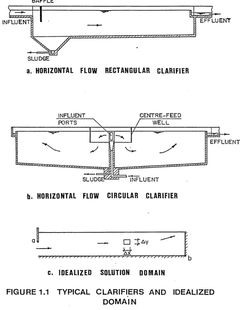
Figure 1.1 Typical Clarifiers and Idealized
D o m a i n ... 207 Figure 2.1 Clarifiers as Solid-Liquid
S e p a r a t o r s ... 208 Figure 2.2 Settling of Suspended S o l i d s ... 209 Figure 2.3 Types of Sedimentation (After L.G. Rich,
Reference 3 ) ... 210 Figure 2.4 Zone and Compression Settling (Adapted
from Reference 2 7 ) ... 211 Figure 2.5 Transport of Sediment into and out of
Element of Unit Volume in Two-Dimensional
Turbulent F l o w ... 212 Figure 2.6 Solid Particle Settling in Turbulent
O p e n - C h a n n e 1 Flow (After Reference 5) . . . 213
Figure 3.1 Defining Sketch, Variable Size M e s h . . . . 214 Figure 3 .2 Three-Time Level F ormulation ...
d t 215
Figure 3.3 Inflow Velocity and Stream-Function
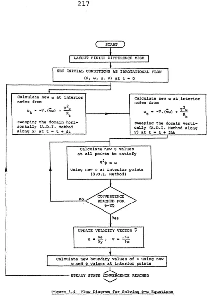
D i s t r i b u t i o n ... 216 Figure 3.4 F low Diagram for Solving Y-m Equations. . . 217 Figure 3.5 Boundary Conditions for C - E q u a t i o n ... 218
Figure 4.1 Effect of Local Courant Number on
Figure 4.8
Figure 4.9
Figure 4.10
Figure 5.1 Figure 5.2
Figure 5.3(a)
Figure 5.3(b)
Figure 5.4(a)
Figure 5.4(b)
Figure 5.5
Figure 5.6
Figure 5.7
Figure 5.8 Figure 5.9
Figure 5.10
Figure 5.11
F o r m u l a t i o n s ) ... C-Distribution (Non-Conservation F o r m u l a t i o n s ) ... Effect of Bottom Boundary Condition on u-Profile ... Effects of n^ and on . . .
Schematic Layout of the Flume. . . . Laser Doppler Anemometer Arrangement
(After Reference 92) ... Longitudinal Velocity Profiles
at X = 0.0, 0.97 ... Longitudinal Velocity Profiles
at X = 2.91,.4.85, 6.5 ... Longitudinal Velocitv Profiles
at X = -0.21, 0.84 ... Longitudinal Velocity Profiles
at X = 2.52, 3.36, 4.62, 5.04. . . . Variation of Eddy Length wit h
Flowrate ... Schematic Layout of Experimental Setup (Dye-Tests)... Typical Flow-Through C u r v e s ,
Hg = 8.25 c m ... . Flow Through Curve for Hg = 3.8 cm . Predicted Flow-Through Curves
at X = 0, 0.063, 1.5, 6.18 ... Experimental ys Predicted
Flow-Through Curves, Hg = 8.25 cm . . . . Experimental ys^ Predicted
Flow-Through Curves, Hg = 3.8 c m ...
Figure A.l
Figure A . 2
Discrete S u s p e n s i o n ... . Typical Settling Column Test
(after Reference 28) . . . . Quiescent Settling Analysis of
Discrete Particles (after Reference 3)
242
243
244
Table 4.1
Table 4.2
Table 4.3
T a b le 4.4
Table 4.5 Table 4.6 T able 4.7 Table 4 .<6
T able 4.9
Table 4.10 Table 4.11
Table 4.12
Table 5.1
T a b le 6.1
Table 6.2
Eff e c t of A t o n S o l u t i o n U s i n g V a r i a b l e
Size M e s h ... 246
Effect of M e s h V a r i a b i l i t y on
S o l ution (I) ... E f f e c t of M e s h Varicibility on
S o l u t i o n (II ) ... E f f e c t of M e s h V a r i a b i l i t y on
S o l u t i o n (III) ... 249 E f f e c t of a on S t e a d y State Solution . . . . 250 Effect of a on T r a n s i e n t S o l u t i o n ... 251 E f f e c t of C__ and R on S t a b i l i t y ... 25 2
N ec
E f f e c t of B o t t o m B o u n d a r y Co n d i t i o n
on S o l u t i o n ...253 E f f e c t of B a f f l e - L i p B o u n d a r y C o n dition
o n S o l u t i o n ...254 Ef f e c t of Eddy V i s c o s i t y on S o l u t i o n . . . . 255 Ef f e c t of Initial C o n d i t i o n on
Steady-S tate V e l o c i t y F i e l d ... . . 256 E f f e c t of Initial C o nditions on
Steady-State C - f i e l d ... 25 7
E q u i p m e n t D e t a i l ... 25 8
S i m u l a t i o n of Removal of N o n - U n i f o r m
Size Discrete S u s p e n s i o n ... 259
E f f e c t of Relative B a f f l e S u b m e r g e n c e
on Removal of S o l i d s ... 2 60
I N T R O D U C T I O N
1.1 O b j e c t i v e
The purp o s e of this d i s s e r t a t i o n is to develop a m a t h e m a t i c a l m o d e l to r e p r e s e n t the s e t t l i n g process in
r e c t a n g u l a r clarifiers. In this study, only the s e t tling b e h a v i o u r of discrete p a rticles is s i m u l a t e d for neut r a l d e n s i t y conditions, i.e., low influent conce n t r a t i o n and no t emperature variations. However, the m o d e l m u s t be such that it can be m o d i f i e d to include changes in tank geometry, dens i t y and susp e n s i o n properties.
1.2 Statement, of the P r o b l e m
In N o r t h America, m o s t of the w a t e r an d w a s t e w a t e r tr e atment plants include at least one stage of s e d i m e n t a tion. M o s t modern s e d i m e n t a t i o n tanks are o p e r a t e d on a continuous flow basis. W h e n e v e r a two-phase mixture, e.g., w a t e r and s u s p e n d e d solids flows under rela t i v e l y q u i e s c e n t conditions, the solids h a v i n g speci f i c w e i g h t h i g h e r than
particulate matter, f locculated impurities and precipitates w h i c h are formed in operations such as coagulation, w a t e r
softening or iron removal. In w a s t e w a t e r treatment plants, s edimentation is used in grit chambers, particulate m a t t e r removal in primary clarifiers and b i o l o g i c a l - f l o e removal in secondary settling tanks. In some instances, coagulants and c o agulant aids m a y b e added to precipitate phosphorus and to increase the settling rate of fine and colloidal s o l i d s .
Sedimentation tanks have been classified according to their use and design criteria, such as grit chambers and primary clarifiers. The difference is m a i n l y in the type and concentration of influent solids and the degree of c larification required. Tanks have also b een clas s i f i e d a ccording to the m a i n flow direction, w h e t h e r horizontal or vertical (upflow t a n k s ) . Horizontal flow tanks m a y be either rectangular or circular. Radial flow clarifiers have b een d e s i g n e d w i t h centre - f e e d and outward flow, or peripheral feed and inward flow.
v a r i a b i l i t y and temperature d i f f e r e n c e s b e t w e e n inflow, tank content and a m b i e n t air temperature.
A m o n g the s uspension char a c t e r i s t i c s w h i c h affect the process are the p h y s i c a l an d chemical characteristics of the
liquid phase such as its temperature, dens i t y and viscosity, and the physical an d chemical c h a racteristics of the solid phase such as the particle size distribution, dens i t y and shape. In addition, the influ e n t conce n t r a t i o n of solids and their flocculant char a c t e r i s t i c s influence the settling v e l o c i t y of the sus p e n d e d matter.
The process of suspended p a rticles settling can be e f f e c t i v e l y analyzed b y treating it as a transport
phenomenon. The analysis consists of two parts, (,i) the hy d rodynamics, (ii) the transport. The h y d r o d y n a m i c
simulation is a prer e q u i s i t e for p r o p e r simulation of convection, diffusion, and resu s p e n s i o n b e h a v i o u r of the sus p e n d e d solids as the flow proceeds along the tank.
1.3 M o t i v a t i o n
W es t Windsor Pollution Control Plant, Windsor, Ontario. A brief review of the literature, at that time, showed that the treatment of the hydrodynamic and transport aspects of this topic were inadequate, although sufficient pertinent
b a ckground material was available.
Early designs of settling basins w ere b ased m a i n l y on experience along wit h some simplified methods of analysis and design. In 1904, Hazen Cl) introduced the concept of o v e r f l o w rate or surface loading. Since then, it has been used extensively as a basis for design. In 1944, Dobbins
C.2) presented a simple transport model which partially
accounted for the effects of turbulence on sedimentation. In 1946, Camp (3) applied Dobbins' model, assuming a
unidirectional flow, to design clarifiers for settling of discrete particles with uniform and non-un i f o r m size
d i s t r i b u t i o n .
Though the design method advanced by Dobbins and Camp
accounts for certain aspects of the transport phenomenon, such as turbulence, it has not been adequate to explain the be h a v i o u r of settling tanks under operating conditions. It
is believed that the mai n reason for this discrepancy is the oversimplified assumption in the hydrodynamic model that the
flow is uniformly distributed both h o r i zontally and
concentration or temperature differences, re-entrainment, shear stresses due to win d on w a t e r surface, and sludge removal m e c h a n i s m on flow pattern.
The large number of factors involved in the settling of suspended particles, discrete or floe, in clarifiers
has led researchers to use black-box type models. Tracer flow-through curves have been utilized to study the
hydraulic behaviour of clarifiers under the assumption that there is a direct correlation between the removal
efficiency and the hydraulic efficiency. Recently, serious doubts have been cast on the validity of flow-through curves as measures of the removal efficiency. For example, these curves do not distinguish between short circuiting due to planwise distribution of flow, i.e., jetting effects, and the vertical flow pattern, i.e., formation of horizontal-axis eddies. It has been indicated (4) that planwise flow distribution seriously affects the removal efficiency.
The progress made in numerical techniques, aided by the increasing capabilities of fast computers, has enabled researchers to solve the governing partial differential
equations under relatively complicated boundary conditions. Models based on a Lagrangian frame of reference and employing
second group of models has tackled the prob l e m through the transport equation in the Eulerian frame of reference. These include hydrodynamic models w i t h varying degrees of
sophistication (7).
A group of Japanese researchers (8, 9) have solved the transport equation using a simple hydrodynamic m o d e l wit h unidirectional flow. They have included the unsteady
nature of the inflow to clarifiers, and allowed resuspension of already settled suspended solids. A l a r i e , et aT CIO, 11)
used a similar approach to simulate circular clarifiers. W ork done by Larsen and Gotthardsson (12, 13) in
Sweden is amongst the m o s t comprehensive research to analyze the b e haviour of rectangular settling tanks. They used a hydrodynamic model based on a finite difference solution
to the equations of motion. The details of their mathematical
model are not available. Larock and Schamber (14) solved the hydrodynamics of a rectangular clarifier using finite
element formulations of the equations of motion. The
geometry of the tank considered is very similar to the flow over cavity. Their work was done concurrently with this project.
It is obvious that a mathematical model which can
properties of suspension w o u l d be v e r y useful. It w ill
allow a rational evaluation of various designs and
suggest effective modifications to remedy malfunctioning.
In addition, it can clarify the role of the various factors involved in the settling process, e.g., the effects of
overflow rate, detention time, suspended solids character istics, inlet and outlet designs and baffling.
1.4 General Approach
The main theme of this dissertation is to predict the removal efficiency of rectangular clarifiers. The prob l e m is tackled by using the convection-diffusion equation of transport. First, the equations of mo t i o n are solved
n umerically to establish the velocity field in the clarifier. Then, the transport equation is solved for the spatial
distribution of suspended solids concentration. The resulting concentrations are then used to construct the iso-concentra tion curves. Finally, the removal efficiency, r, is computed from r = 1 - , where and are the influent and effluent suspended solids concentrations respectively.
The derivation of hydrodynamic sub-model is carried out
in three steps: (i) setting up the governing equations, Cii) identifying the solution domain, and (.iii) selecting the numerical scheme. Flo w in a settling basin involves
two phases under relatively complicated boundary conditions. The f l o w is considered three-dimensional in the inlet zone, b u t downstream from the inlet zone, a two-dimensional
representation m a y be adequate. Density gradients due to temperature or concentration variation may affect the flow pattern.
In the present problem, the stream function-vorticity formulations are used. The unsteadiness term in the
vor t i c i t y equation is retained to control computational stability and the steady state solution is obtained as the asymptotic time limit of the unsteady equation. A two-dimensional representation is employed in this phase of the study because, although the storage of computer could handle a three-dimensional analysis, it w o u l d be a special job wit h very poor turn-around. Also, the CPU time (execution time) per run w o u l d be very excessive. This results in limiting the simulation to the settling zone. A simple turbulence model using a constant eddy viscosity is incorporated and its adequacy is assessed. The hydrodynamics is decoupled from the transport equation by excluding vorticity generated from density gradients. This restricts the simulation to neutral or near neutral density conditions. The m o d e l must
be such that it can be readily m o d i f i e d to simulate other special conditions.
this study. The geometry is typical of the settling and
outlet zones in m a n y rectangular clarifiers and mos t centre-feed circular clarifiers. It is w orth mentioning that the mathematical model is general enough to handle other geometries after making appropriate changes in
bo u ndary conditions.
The governing differential equations are not
'amenable to analytical solutions under the given boundary
conditions. Hence, the solution has to be obtained
numerically, for example, b y using either a finite difference
scheme or a finite element method. In the present study, the finite difference scheme is considered more appropriate
because : (i) its treatment is considerably simpler for the rectangular geometry involved, (ii) it requires less computer storage, and (iii) there is a vast literature on its application to other recirculating flow problems (15, 16,) , e.g., backward facing step problem and flow over
cavity.
The second part of the simulation involves solving the convection-diffusion equation with an additional sink term that accounts for the settling v e l ocity of the solids
relative to the liquid. The settling velocity is assumed constant with time and space. Thus, the m odel is capable of simulating discrete particles settling. Flocculant
quasi-discrete or by incorporating an appropriate algorithm to change the settling velocity wit h space to account for the effect of flocculation on the settling velocity. An appropriate boundary condition along the tank bottom can be utilized, to simulate resuspension of already settled p a r t i c l e s .
Model v e r i f i c a t i o n , calibration and validation
represents the last step in developing a simulation model. This has been done in two stages: (i) numerical testing or model verification (17), and Cii) parameter calibration using experimental data. The numerical testing ensures removal of anomalies from the simulation and perfection of the scheme before the actual calibration is done. Two
sets of experiments have been conducted to calibrate the
m o d e l parameters: (i) velocity measurements for the calibration and validation of the hydrodynamic part, and
(ii) dye tests for the validation of the transport model. Neutral density tracers, such as dyes, have been used instead of actual sediment because of the simplicity of these tests as opposed to sedimentation tests. It is believed that if the model adequately simulates the
transport of dye which could be regarded as sediments with zero settling velocity, it should be capable of
BACKGROUND AND REVIEW OF THE LITERATURE
2.1 General
In sedimentation tanks, the mixture of water and impurities enters from the inlet zone and, as it proceeds towards the effluent zone, the suspended solids settle downward to the sludge zone due to the gravitational effect, as shown in Fig. 2.1. Most modern clarifiers are operated on a continuous flow basis and the factors
affecting the removal process can be divided into three groups as explained in Fig. 2.2: Ci) the characteristics of the suspended solids and the transporting liquid,
(ii) hydrodynamic parameters in continuous flow operation,
and (iii) field conditions.
2.2 Settling Characteristics of Suspended Solids (Types of S e d i m e n t a t i o n )
Particles settle from suspensions in different manners, depending upon the suspension concentration and the
flocculating properties of the particles. Four types of
sedimentation have been identified : (i) type-I sedimentation, (ii) type-II sedimentation, (iii) zone settling, and (iv)
settling regime are illustrated in Fig. 2.3. Alternatively, the settling patterns can be classified, o n the basis of solids concentration in the suspension, as: (i) free settling when particles settle individually at different rates in a dilute suspension, (ii) hindered settling when the settling of particles is influenced by the presence of other particles, and (iii) compression settling whe n the rate of settling is reduced due to the physical contact
between p a r t i c l e s .
The four types of sedimentation are described b elow w ith emphasis on the procedure to obtain necessary
information on the settling velocities of suspended solids.
Such information is obviously a prerequisite for simulating the settling process w i t h i n the clarifier.
2.2.1 Type-I Sedimentation
Type-I sedimentation is concerned with the settling of non-flocculating, discrete particles in a low concentration suspension. The settling of such particles is unhindered by the presence of other particles and every particle retains its individual characteristics. When a discrete particle is released in a quiescent fluid, it accelerates until the
fluid drag reaches equilibrium with its effective weight. After that, the particle settles out at a constant velocity called the fall or terminal or settling velocity. This
and v i s c o s i t y) , and particle characteristics (size, shape,
density, o r i e n t a t i o n ) . Khattab (18) presented a review of the various factors involved in discrete settling.
Clarifiers that exhibit type-I sedimentation are modelled by assigning a constant settling velocity during the
settling process.
A typical suspension of particulate matter m a y have a wide range of particle sizes. Thus, the suspended solids
involved have a corresponding range of settling velocities. A frequency distribution of settling velocities or a
settling-velocity analysis curve (19) should be determined. This curve can be constructed by two different ways; (i) by the use of sieve analysis and h y drometer tests combined w i t h the equilibrium equation that relates settling velocity w i t h particle size (3, 20), or (ii) by use of a settling
column as explained in Appendix A.
2.2.2 Type-II Sedimentation
Suspended solids in domestic and industrial wastewaters do not act as discrete particles (21). In general these solids are comprised of particles of different sizes and surface characteristics. Under quiescent conditions, large particles having h i g h settling velocities overtake and
formed particles exceed the settling velocities of the
parent particles.
The extent to w hich flocculation occurs in a settling
tank is dependent on the opportunity for contact, which varies w i t h the range of particle sizes, the concentration
of particles, the depth of the tank, and the velocity gradients in the tank w h e r e b y particles in regions of higher velocity overtake and coalesce wit h particles in regions of lower velocity (3). As particles grow, their shear resistance decreases and w h e n the shearing strength of the particle is exceeded by the applied shear due to
local velocity gradients, the particle ceases to grow. The dynamics of growth and breakage of floes in presence of fluid shear has been reported by various writers (3, 22, 23, 24) .
Because there is no adequate mathematical relationship to determine the effect of flocculation on the rate of
Concentrations are plotted w i t h time and depth and the so-called iso-removal lines are constructed. Tliese iso-removal lines are then analyzed to obtain the necessary information
regarding the settling characteristics.
Appendix A presents a brief summary of the test
procedure, and the various methods of analysis. McLaughlin (2 6) proposed a similar settling column test along with a m o d i f i e d m e t h o d of analysis that yields suspension settling
characteristics in a format more convenient for a
sophisticated transport model.
2.2.3 Zone and Compression Settling
The settling characteristics exhibited by concentrated
suspensions or sludges, where both zone settling and compression usually occur, differ from those of dilute
suspensions. In the latter case, mo s t l y discrete settling. Type-I sedimentation, or flocculant settling, Type-II
sedimentation, are encountered. Zone and compression settling are normally observed in clarifiers of activated sludge or flocculated chemical suspensions where solids concentration exceeds 500 m g / L (22, 27, 28). Although this dissertation is primarily concerned with the clarification of low
concentration suspensions, zone and compression settling are briefly outlined, to illustrate the limits on any
W h e n solids concentration is high, particles settle in close proximity, their v e l o c i t y fields interfere and the settling is hindered. In this case, the settling v e l o c i t y of the suspension as a w h o l e is less than the settling
v e l o c i t y of the single particles. If the suspension is n o n - f l o c c u l a n t and has a wide range of size distribution, the bul k settling rate w i l l be betw e e n the fall v e l o c i t i e s of the fastest and the slowest particles (13).
Zone and compression settling of a given sludge sample can be studied by c onsidering its settling b e h a v i o u r in a settling column. A one-litre g r a d u a t e d cylinder is
c onsidered to be satisfactory in this case (22). Initially, the solids c o n c entration has to be u n i f o r m throu g h o u t the column as shown in Fig. 2 . 4 ( a ) . If the concentration is hig h enough, the sludge starts to settle out wit h a distinct
interface (interface-1) between the mass of the settling sludge and the clarified liquid above. The zone b e l o w the clarified liquid is called the interfacial zone (27) and the solids concentration in this zone is u n i f o r m and equal to the initial concentration.
The sludge p a rticles in this zone settle as a blanket, m a i n t a i n i n g the same relative position w i t h resp e c t to
settling velocity can b e obtained by observing the rate of subsidence of interface-1 w i t h time, as shown in Fig. 2.4(a). As the settling proceeds, the solids on the b o t t o m of the column build up at a constant rate. Subsequently, a
transition zone is observed in w h i c h the settling velocity decreases due to the increase in solids concentration. The concentration of solids in the zone settling layer remains constant until interface-1 meets wit h the rising layers of compressed s o l i d s . A t this time, t^ in Fig. 2.4(c), the
transition zone disappears and the column displays two zones: (i) clarified liquid zone, and (ii) compression zone. The compression zone exhibits a u n i f o r m concentration called the critical concentration, C2 . With time, compression
takes place and sludge begins to thicken, eventually reaching an ultimate concentration, C^.
In summary, clarifiera handling suspensions of high concentrations experience zone settling and compression.
The settling velocity in this case, depends on the unhindered settling rates of the solids involved as well as the sludge concentration. Larsen and Gotthardsson (13) used the
''s = ''so 2-1 where
Vg = suspension settling rate;
V g ^ = terminal settling V e l o c i t y at infinite dilution;
C = m ass concentration of solid particles ; and
a = a constant depending on sludge properties and to be determined using sludge volume index.
2.3 Hydrodynamics of Settling Tanks (Governing Equations of M o t i o n )
2.3.1 Preamble
F low in a settling tank represents a stratified, two-phase, turbulent flow. The equations of motion of
two-phase flow are the obvious starting point for a comprehensive simulation. In similar sediment-related problems, a simple, but a d e q u a t e ,'approach has bee n frequently used where the
liquid-phase simulation is decoupled from the solid-phase simulation. In this approach, it is assumed that the presence of solids does not affect the mechanics of flow of the liquid phase except for its effects on turbulent mi x i n g and density stratification. Hence, flow is treated
as a single-phase flow to establish the velocity and
turbulence fields in the clarifier. This section introduces the hydrodynamic part of the simulation. Subsequently, based
is transported through th_e clarifier using the convection-diffusion equation, as described in Sec. 2.4.
The hydrodynamic simulation of any flow configuration involves the following steps; (.i) identifying the
computational domain, (.ii) deriving the appropriate forms of the governing equations, (iii) choosing a suitable mesh system. Civ) formulating the selected numerical scheme,
(v) defining the boundary conditions, (vi) selecting the
initial conditions, (vii) developing the solution procedure, and (viii) determining the convergence and stability of the resultant scheme. The computational domain for the present problem is shown in Fig. 1.1(c). Steps (ii) and (v) are reviewed in the following sections. Other steps are
described in Chapter 3 where the problem formulation is presented.
2.3.2 Navier-Stokes Equations
Fluid flow is generally governed by a set of coupled partial differential equations which are statements of the conservation of mass, linear m o m e n t u m and energy. In the present problem, isothermal conditions are assumed and only
the continuity equation (conservation of mass) and the equations of motion (conservation of momentum) need to be treated. For the fluid element shown in Fig. 1.1(c),
CNavier-Stokes) and the continuity equation (29, 30) are
vV^u + 2.2
2 F 2 3
+ vV V + y l ü + + V iü + w _ 1 3p
^t 3x 3y 3z P 3x
3v
+ u ^ + V 3v + w IV = _ i i P
3t 9x ay 3z p ay
3w u ^
+ V 3w + w 3w _ - 1 IE
3t 3x ay 3z P az
+ ^ 4 . 3w = 0 3x 3y 3z
2.4
2.5
where
2 2 2 2
V = Laplacian operator = j- + j-3x 3 y 3 z
u,v,w = X - , y-, z- components of velocity respectively;
p = pressure;
F ,F ,F = X - , y-, z- components of external body force on X y z
element per unit mass ;
V = mol e c u l a r kinematic viscosity;
x,y,z = coordinates of element in x,y,z directions ; and t = time.
Equations 2.2 to 2.4 are the x,y,z - vector components of Newton's second law of motion, F = ma. In these equations, it is assumed that fluid is incompressible, with constant
external body force, (F ,F ,F ), is the gravitational
X y X
force on the element per unit mass. Equation 2.5 is a statement of mass balance over the element. The equations are written in an Eulerian frame of reference, i.e., a
space-fixed reference through w h i c h the fluid flows (29, 30). Under laminar flo w conditions, these equations offer a complete solution to the viscous flow problem c o n s i d e r e d .
2.3.3 Reynolds Equations
In a turbulent flow, all flow parameters such as
velocity and pressure are randomly fluctuating about mean or statistical average values (31). These mean motions do not satisfy the Navier-Stokes equations (3 2).
The instantaneous mo t i o n does obey the equations and, in principle, methods exist for solving them directly.
However, proper resolution of small scale turbulent motion,
which ma y be about one m i llimeter in size, would require an impractical fine computational mesh. The resulting solution, in such a case, w o u l d be of little practical
value since it would describe the randomly varying flow domain at only one instant. It is the mean motion, along with appropriate statistical characteristics of the
turbulent fluctuations, that are normally of interest
A turbulent flow is effectively studied by separating
the fluid motion into a m e a n m o t i o n and a turbulent fluctu ating motion. Flow variables such as velocity, u, are d e composed into a statistical average velocity, u, and a turbulent fluctuating velocity, u ' , (31, 33), i.e.,
u = Ù + u' 2.6
Substituting for all flow variables using expressions similar to Eq. 2.6 into the Navier-Stokes and the continuity equations, and taking the m e a n values of the equations
according to Reynolds rules of averaging (31, 3 2), a new set of equations is obtained. The resulting equations, for incompressible, Newtonian fluid, usually referred to as Reynolds equations, read
3t 9x 9y 3z P 3x 3x 3 y
+ 2 2.7
3Z
3Y. + ü 3 z + v 2 i + w S i = _ 1 m
3t 3x 3y 3z p 3y 3x 3y
-^3( - V W ) 2 .8
8z ^
+.Ü + V ^5 + w ^
3t 3x 3y 3z P ÔZ g
where the overbar represents the mean value and the prime, the turbulent fluctuations. Equations 2.7 to 2.9 differ from E q s . 2.2 to 2.4 in the presence of certain terms added to the mean values of stresses due to viscosity. These additional stress-like terms are called Reynolds or
eddy stresses.
2.3.4 Mathematical Models of Turbulence
The solution of Reynolds equations represents properly the turbulent flow field. However, the number of equations
is less than the number of unknowns; the mean pressure, the mean velocity components and the Reynolds stresses. In order to overcome this so-called "closure problem" further hypotheses about Reynolds stresses m u s t be made, i.e., a
turbulence model is required. According to Launder and Spalding (34), a turbulence model means "a set of equations which, when solved w i t h the mea n - f l o w equations, allows the
calculation of the relevant correlations and so simulates the behaviour of real fluids in important aspects".
the mea n motion rate of strain by an effective, apparent or eddy kinematic viscosity, e^.
.3Ü . 9v
-u'v' = e + LJL) 2.11
^ 3y 3x
is also referred to as the m o m e n t u m eddy diffusivity or transfer coefficient.
The problem can n o w be solved, once a satisfactory
relation is chosen to estimate the scalar kinematic eddy viscosity, within the flow field. Models of the first group, vary in sophistication in calculating and the
models of constant eddy viscosity have been used frequently. An improved version of these models replaces the scalar
by a second-order tensor for the eddy viscosity (31). This approach is wi d e l y used in pollution dispersion problems, e.g., in rivers, where different values of are assigned to various directions, i.e., vertical, transverse, and
longitudinal (33).
Other models use algebraic formulae for e^, e.g.,
Prantl's mixing length hypothesis, and Von-Karman's
similarity hypothesis (35). Also, there are complex models which solve for one or m o r e differential equations to
estimate . The Kinetic energy-dissipation or K-e model
"stress transport models" because they evaluate the Reynolds stresses using stress transport equations, mostly of the differential type. An example of an elaborate model from this group is the Kolavandin model (34) w hich involves solving 28 turbulence differential equations for the case of a three-dimensional problem and 20 equations for a two-dimensional one.
Turbulence models are judged (34) on the basis of their accuracy, width of applicability, simplicity and total economic expenditure, bot h in terms of manpower and computing time. Launder and Spalding, in their lectures on mathematical models of turbulence (34),
commented that "the b e s t m odel of turbulence will differ according to the problem under consideration," and they pointed out that "the more direct knowledge of the flow, the greater is the chance that a simple description of turbulence can be made to s u f f i c e " . In addition, any turbulence model, regardless of its sophistication, has to be calibrated and the task of optimising the constants and functions increases very rapidly wit h the number of
e q u a t i o n s .
In the present problem, the "mixed^region" (38) flow domain includes a wall jet, a shear layer, a large recirculating flow region and a sink-dominated region
equations of fluid motion, Eqs. 2.7 - 2.10, can be difficult for such a domain, even w h e n considerations of turbulence are totally absent. Hence, a constant eddy viscosity model has been selected, at this stage, where an average effective v iscosity is assigned to the whole computational domain.
With such a simple turbulence m o d e l , it is hoped that
problems associated w i t h the numerical scheme and boundary conditions can be identified and solved independently of turbulence-related problems. The full implementation of a complex turbulence model such as the K-e model would
almost double the computational time. However, a relatively efficient solution could be obtained by incorporating the K-e during the latter stages of the present model.
A turbulence model, b ased on the scalar constant eddy
viscosity, often results in velocity profiles similar to those of laminar flow. To correct partially for this effect, w i t h o u t using a more complex turbulence model, a partial-slip boundary condition can be used along the clarifier bed, as w ill be explained later.
2.3.5 Incompressible Flow Equations (Primitive Equations)
variable. However, c o m p u t a t i o n a l fluid dynamicists (40, 41) h ave r e p o r t e d that steady state solutions can be mor e
successfully o b t a i n e d as being the a s ymptotic time limit
of the u n s t e a d y e q u a t i o n b e c a u s e of improved compu t a t i o n a l stability. Frankel (16) dis c u s s e d the i n t erpretation of the t i me-step equations as iterative relaxations of the steady state e q u a t i o n s . For m o r e details on the use of the u n s t e a d y e q u a t i o n to solve steady state problems, the
reader is r e f erred to Cheng's review o f numerical solutions
of Navie r - S t o k e s equations (38).
2.3.7 C o n s e r v a t i o n F orm
E q u a t i o n 2.16 is r e f e r r e d to as the "non-conservation" form of the v o r t i c i t y transport equation (40). It can be recast in a di f f e r e n t but e q u i v a l e n t form to take advantage
of the "conservation property" d i scussed by Roache (40). Tf the slightly m o d i f i e d v e r s i o n of the c ontinuity equation
+ iZ, . ^ 1 5 + = 0 2.19
9x 3y 3x 3y
is added to bot h sides of Eq. 2.16, then the so-called
"conservation form" of the v o r t i c i t y transport equation is o b t a i n e d
= . l i S Ë l . ^ ,2^ 2.20
for the Reynolds stresses by expressions similar to Eq. 2.11, the equations of motion and the continuity equation for a two-dimensional case can be reduced to
+ e V u + F._ 2.12
at 9x By p ax
+ F 2.13
at ax ay p Sy ™ ^
— + — = 0 2.14
3x 3y 2
where V is the two-dimensional Laplacian operator. The overbars on the various terms have been omitted for sim plicity, yet, all terms represent m ean values. The term,
is the effective kinematic eddy viscosity and the
m o l e c u l a r kinematic viscosity has been neglected compared to its turbulent counterpart. According to Hinze (31),
Eqs. 2.12 and 2.13 are not strictly correct unless the trace of the stress tensor is subtracted; yet this difference is immaterial in a simple model (39) and can be neglected. Equations 2.12 - 2.33 are similar to Navier-Stokes e q u a tions 2.2 - 2.4, except that the relatively small molecular kinematic viscosity, v, has been replaced b y the scalar kinematic eddy v i scosity (generally Gj^>>v) and that all
the flow quantities have been averaged.
The equations are written in terms of the primitive
"primitive equations" (40). Equations 2.12 and 2.13 are second order due to the stress terms and are non-linear due to the quadratic convective inertia terms. Hence, a hydrodynamic simulation using these equations involves
solving three simultaneous (coupled) non-linear partial differential equations in three unknowns, u, v, p.
2.3.6 Stream Function-Vorticity Transport (Y-w) Equations
In simulating settling tanks, the pressure distri bution per se is not required. Hence, the equations of motion can be recast in another format where the pressure is eliminated and only one transport equation needs to be treated. The pressure, p, can be eliminated from Eqs. 2.12, 2.13 (40) by first cross-differentiating Eq. 2.12
wit h respect to y and Eq. 2.13 with respect to x and then subtracting. Noting that the gravitational body forces, (F^, F ^ ) , have zero derivatives with respect to
5^ and x respectively, and defining the vorticity, ûj as
Û) = — - — 2.15
3 y 3x
the following parabolic vorticity transport equation (oj-Equation) is obtained
+ e + i f f , . 2.16
Defining the stream function, Y, by
^ = u and ^ = - V. 2.17
Equation 2.15 is rewritten as
2.18(a)
2 2
ax ay
or
V^Y = m 2.18 Cb)
w hich is an elliptic Poisson type equation.
The vorticity transport equation, Eq. 2.16, consists of (i) the unsteady or local inertia term, |~, (ii) the convective or advective terms, u | ^ and v ^ , and (iii) the
2
diffusion terms, w. The equation states that the rate of change of w is the difference between the net vorticity convected along with the flow in or out of the element and the vorticity diffused due to gradient in or out of the
element. The vorticity is generated from walls or sudden changes in flow direction. Because of the unsteady term, the m-equation represents an initial-value problem, wherein the solution is started from some initial conditions.
The present investigation is concerned with clarifiers under steady or near steady state conditions, where can be set to zero in Eq. 2.16. This approach is often used in
Although Eqs. 2.20 and 2.16 are m a t h e m a t i c a l l y two equivalent differential e q u a t i o n s , this is not true when the equations are differenced. The finite difference
analog of the conservation form; Eq. 2.20, has been shown to possess the conservative p r o p e r t y as it preserves the integral Gauss divergence p r o perty of the c o n tinuum
equation (Ref. 40, pp. 30). W h e n n e i g h b o u r i n g volumes are summed, the contributions on their common b o u n d a r y cancel identically, so that the integral conservation laws retain the same form.
2.3.8 Initial and B o u ndary Conditions for (Y-m) Equations
In the solution of any time dependent partial d i f ferential equation, it is nec e s s a r y to specify the initial state of the flow domain an d the conditions at its b o u n d aries. W hen the u n s teady equation is used to obtain a steady-state solution, a plausible initial solution is n o r mally assumed, e.g., fluid initially is at rest. The effect of the initial conditions on the final solution,
when a finite-difference scheme is use d (40) , is r elatively small compared to the same effect in a finite-element formulation (39).
partial differential equations w h i c h describe the phenomenon. On the dominant importance of computational boundary con ditions , Roache c o m m e n t s ,"All the fantastic flow patterns of common gases and liquids are solutions of the same pa r tial differential equations, the Navier-Stokes equation. The flows (solutions) are distinguished only by boundary and initial c o n d i t i o n s , and by the flow parameters such as R .", where R is a characteristic Reynolds number,
e e
This section introduces the possible methods for
treating the various boundary conditions (for both Y and cu equations) involved in the computational domain under in vestigation. Before proceeding, it is important to mention
that there are two mesh systems. In the first mesh system, Y and m are calculated at the same nodes, and nodes can
lie along the w a l l s . The second mesh system includes space-staggered meshes, and s h i f t e d - m e s h e s , in which some flow variables are defined at one set of nodes, and other variables in a mesh dislocated from the first, in a certain way. The first mesh system has been used w i d e l y b y man y
researchers, in similar-type recirculating flow problems (Ref. 40, pp. 148) and is incorporated in the present m o d e l .
w h e r e a constant Y can also be assigned. Thus at the free surface, the v e r t i c a l v e l o c i t y com p o n e n t (normal to the surface) is zero, and the horizontal, along the surface, component is free to develop. Inflow and o u t f l o w b o u n d aries are o f t e n p r e s c r i b e d as D i r ichlet boundaries w h e r e Y-values are o b t ained b y i ntegrating an assu m e d or m e a s u r e d
v e l o c i t y distribution.
Unlike stream function b o u n d a r y c o n d i t i o n s , v o r t i c i t y b o u n d a r y conditions are d i f ficult to evaluate and yet
c rucial to a successful simulation. The v o r t i c i t y t r a n s port equation, Eq. 2.20, o n l y determines h o w co is convected and diffused, w h i l e the total w is con s e r v e d at the i n
terior n o d e s . At inflow b o undaries w m a y be flowing into the domain and it is also gen e r a t e d at solid w a l l s . This f lux of v o r t i c i t y is c o nvected and/or diffu s e d in the domain, thus shaping the flow pattern.
In the absence of applied shear such as w i n d shear and temperature gradients, v o r t i c i t y at a free fluid s u r face can be shown to be zero (42). V o r t i c i t y values at inflow and outflow boundaries are deduced from the given v e l o c i t y distributions. At sharp-concave corners, such as p o i n t b in Pig. 1.1(c), m is zero. Actually, w at such a point does not enter into the calculations w h e n a 5-point difference equation is used at interior points.