CERJAK, JASON ROBERT. Evaluation of MM5 Forecasts of Near-Surface Parameters: Sensitivity to Land-Surface Parameterization and Planetary Boundary Layer Schemes. (Under the direction of Dr. Gary Lackmann.)
The specific purpose of the research is to evaluate the performance of the MM5 model in the forecasting of near-surface parameters, such as 2-meter temperature, 2-meter dew point, and 1000-850 mb thickness. The evaluation will include a comparison of the MM5 against the Eta model, and a comparison of the forecasting skill of the MM5 with three different land-surface parameterization schemes. Three different soil moisture scaling techniques will be applied to the MM5, and their forecasts will be evaluated against observations taken from 7-9 December 2001.
BOUNDARY LAYER SCHEMES
by
JASON ROBERT CERJAK
A thesis submitted to the Graduate Faculty of North Carolina State University in partial fulfillment of the requirements for the Degree of
Master of Science
MARINE, EARTH, AND ATMOSPHERIC SCIENCES
Raleigh 2002
APPROVED BY:
_____________________________ ____________________________
Jason Cerjak was born in Cleveland, Ohio, on February 13, 1978. His life was tied with meteorology even before his birth. On January 25, 1978, the worst winter storm in the recorded history of Cleveland weather, the great Cleveland Superbomb, or the “White Hurricane” as it was called in his hometown, ravaged much of the lower Great Lakes. Mr. Cerjak went to Brentmoor Elementary School, Ridge Junior High School, and Mentor High School all in Mentor, Ohio, and
This thesis was supported through a research grant funded by the Capitol Broadcasting Company.
I would like to thank all of my parents: my father, Thomas Cerjak, my stepmother, Judy Williams, my mother, Sharon Faber, and my stepfather, Richard Faber. It was only through their support and understanding that I was able to attend and complete my Master’s Degree. If not for my family, then I would not have
accomplished so much.
I would like to thank my primary advisor, Dr. Gary Lackmann. Dr.
Lackmann’s understanding of academic research enhanced not only the quality of my own research, but also my academic, career, and personal matters as well. I would not be as prepared for my career in the atmospheric sciences if not for the guidance of Dr. Lackmann. Also to Dr. Jerry Davis and Dr. Al Riordan for serving on my thesis committee. Dr. Davis provided invaluable assistance on the statistical and technical issues of my research. This thesis would not have the scientific strength if not for the assistance provided by Dr. Davis. Dr. Riordan provided invaluable insight on the process of thesis writing, and his valuable input enabled me to draft this thesis with a high level of quality.
Modeling Center. Mr. McHenry and his staff were extremely helpful by providing the computing resources necessary to operate the MM5 model. Needless to say, if not for Mr. McHenry’s staff, this thesis would not be possible.
I would like to thank the members of my research lab (Wyat Appel, Michael Brennan, Keith Contre, Heather Reeves, Scott Kennedy, Wendy Sellers, Mike Trexler, and Richard Yablonsky) for their assistance in the creation of this thesis. Each in their own way has added some input into this thesis, and the quality of this thesis would not be the same if not for my colleagues from the forecasting lab.
I would also like to thank Heather Arkinson, Jessica Blunden, Bob Bright, Mark Modrak, John Petters, and Nick Witcraft. These people were some of the best friends that I have ever known, without them, my life would not be as enriched, and I would not be the person I am today.
Page
LIST OF FIGURES ... vii
1. INTRODUCTION ... 1
1.1. Project Description ... 1
1.2. Link Between Land Processes and the PBL ... 1
1.3. Land-Surface Scheme Background ... 4
1.4. Land-Surface Scheme Comparison ... 9
1.5. PBL Scheme Comparison ... 16
1.6. Discussion ... 23
1.7. Thesis Organization... 27
2. METHODS... 28
2.1. Observation Stations ... 28
2.2. Types of Data Included... 28
2.3. Model Configuration and Physics... 30
2.4. Changes to the MM5 During the Study Period... 32
2.4.a. Soil Moisture Scaling Technique ... 33
2.5. Numerical Methods Utilized... 33
3. MODEL COMPARISON ... 35
3.1. Observed Weather Conditions ... 35
3.2. Results from Model Comparison ... 35
3.2.a. 2-meter Temperature ... 35
3.2.b. 2-meter Dew Point... 44
3.2.c. 1000-850 mb Thickness ... 49
3.3. Discussion ... 52
4. PERIOD COMPARISON ... 54
4.1. Methodology ... 54
4.2. Meteorological Setting of the Study Periods ... 54
4.3. Results from Period Comparisons... 56
4.3.a. 2-meter Temperature ... 56
4.3.b. 2-meter Dew Point... 59
4.3.c. 1000-850 mb Thickness ... 62
4.4. Discussion ... 65
5. METEOROLOGICAL SETTING OF 7-9 DECEMBER 2001 ... 68
5.1. Synoptic Setting... 68
6.1. Methodology ... 80
6.2. 2-meter Temperature... 80
6.3. 2-meter Dew Point... 83
6.4. 1000-850 mb Thickness ... 86
6.5. Discussion ... 88
7. SENSITIVITY TEST: 7-9 DECEMBER 2001... 90
7.1. Rationale ... 90
7.2. Methods ... 90
7.3. The Diurnal Cycle ... 91
7.4. Discussion ... 102
8. THESISSUMMARY ... 104
CHAPTER 1
Figure 1.1 Drought index for the United States as calculated by the U.S.
Drought Monitor for 15 August 2000 ... 21 Figure 1.2 Drought index for the United States as calculated by the U.S.
Drought Monitor for 11 September 2001... 22 Figure 1.3 Monthly precipitation and precipitation climatology for Arizona (in
2000) and North Carolina (in 2001)... 22 Figure 1.4 Drought index for the United States as calculated by the U.S.
Drought Monitor for 11 December 2001... 23 Figure 1.5 Relevant strengths and weaknesses of the four PBL schemes
studied by Bright and Mullen (2002) and the five land-surface
schemes as compared by Chen et al. (1996) ... 26 CHAPTER 2
Figure 2.1 Map of observation points ... 29 Figure 2.2 Map of MM5 model domains ... 31 CHAPTER 3
Figure 3.1 1200 UTC temperature forecasts and observations every day at
RDU in the study period ... 36 Figure 3.2 2400 UTC temperature forecasts and observations every day at
RDU the study period ... 37 Figure 3.3 1200 UTC dew point forecasts and observations every day at
RDU in the study period ... 38 Figure 3.4 2400 UTC dew point forecasts and observations every day at
RDU in the study period ... 39 Figure 3.5 24-hour precipitation forecasts and observations every day at
RDU in the study period ... 40 Figure 3.6 Mean, Standard Deviation, and Variance of 2-meter temperature
forecast biases from the Coarse MM5, Fine MM5, and Eta
models from the entire study period ... 42 Figure 3.7 Mean, Standard Deviation, and Variance of 2-meter temperature
forecast errors from the Coarse MM5, Fine MM5, and Eta
models from the entire study period ... 42 Figure 3.8 Temperature biases from the entire study period ... 42 Figure 3.9 Temperature errors from the entire study period ... 43 Figure 3.10 Same as Figure 3.6, except the data is for 2-meter dew point
forecast biases ... 46 Figure 3.11 Same as Figure 3.7, except the data is for 2-meter dew point
forecast errors ... 46 Figure 3.12 Dew point biases from the entire study period ... 47 Figure 3.13 Dew point errors from the entire study period ... 47 Figure 3.14 Same as Figure 3.6, except the data is for 1000-850 mb
thickness forecast biases ... 50 Figure 3.15 Same as Figure 3.7, except the data is for 1000-850 mb
Figure 4.1 Daily averages of observed 2-meter temperature, 2-meter dew
point, 1000-850 mb thickness, and rainfall, separated by period... 55
Figure 4.2 2-meter temperature biases by period ... 57
Figure 4.3 2-meter temperature errors by period ... 58
Figure 4.4 2-meter dew point biases by period ... 60
Figure 4.5 2-meter dew point errors by period ... 60
Figure 4.6.a Mean, standard deviation, and variances of dew point biases from Period 1 ... 62
Figure 4.6.b Mean, standard deviation, and variances of dew point biases from Period 3 ... 62
Figure 4.6.c Mean, standard deviation, and variances of dew point errors from Period 1 ... 62
Figure 4.6.d Mean, standard deviation, and variances of dew point errors from Period 3 ... 62
Figure 4.7 1000-850 mb thickness biases by period ... 63
Figure 4.8 1000-850 mb thickness errors by period ... 64
CHAPTER 5 Figure 5.1 Eta model analysis at 0000 UTC on 7 December ... 69
Figure 5.2 Eta model analysis at 0000 UTC on 8 December ... 70
Figure 5.3 Eta model analysis at 0000 UTC on 9 December ... 71
Figure 5.4 Eta model analysis at 1200 UTC on 9 December ... 72
Figure 5.5 Observed skew-T from GSO at 0000 UTC on 7 December... 73
Figure 5.6 Observed skew-T from GSO at 0000 UTC on 8 December... 73
Figure 5.7 Observed skew-T from GSO at 0000 UTC on 9 December... 74
Figure 5.8 Observed skew-T from GSO at 1200 UTC on 9 December... 74
Figure 5.9 Observed 2-meter temperatures at all five sites ... 77
Figure 5.10 Observed 2-meter dew points at all five sites ... 77
Figure 5.11 Observed 1000-850 mb thickness at all five sites ... 78
CHAPTER 6 Figure 6.1 Temperatures from all sites from 7-9 December... 81
Figure 6.2 Temperature biases in model runs for 7-9 December... 82
Figure 6.3 Temperature errors in models runs for 7-9 December... 82
Figure 6.4 Dew points for all sites from 7-9 December ... 84
Figure 6.5 Dew point biases in model runs for 7-9 December ... 85
Figure 6.6 Dew point errors in model runs for 7-9 December ... 85
Figure 6.7 1000-850 mb thickness for all sites from 7-9 December... 87
Figure 6.8 1000-850 mb thickness biases in model runs for 7-9 December ... 87
Figure 6.9 1000-850 mb thickness errors in model runs for 7-9 December... 88
Figure 7.1 Table of observed and analyzed soil moisture at 0000 UTC 7
December 2001 ... 90 Figure 7.2 Soil moisture scaling reduction factors in the four soil layers for
each MM5 model run in the forecast period from 7-9 December
2001... 91 Figure 7.3 2-meter temperature observations and forecasts from the three
MM5 model runs from 0000 UTC 7 December through 0000 UTC
9 December. ... 92 Figure 7.4 Forecasts of sensible heat flux from all three MM5 model runs... 93 Figure 7.5 2-meter dew point observations and forecasts from the three
MM5 model runs from 0000 UTC 7 December through 0000 UTC
9 December ... 94 Figure 7.6 Forecasts for latent heat flux from the three MM5 model runs... 95 Figure 7.7 Forecasts of shortwave radiation by the three MM5 model runs
for 7-9 December... 96 Figure 7.8 Forecasts of total column cloud mixing ratio from each MM5
model run from 7-9 December ... 97 Figure 7.9 Observed cloud cover every hour at RDU from 0000 UTC 7
December 2001 through 9 December 2001 ... 98 Figure 7.10 1000-850 mb thickness observations and forecasts from the
three MM5 model runs from 0000 UTC 7 December through
0000 UTC 9 December... 99 Figure 7.11 Forecasts of boundary layer height from the three MM5 model
runs for 7-9 December...100 Figure 7.12 Highly Scaled MM5 forecast sounding for RDU at 1800 UTC 7
December 2001 ...101 Figure 7.13 Eta model analyzed sounding for RDU at 1800 UTC 7 December
2001...101
1. Introduction
1.1. Project description
This thesis project is based upon the evaluation of the performance of the Penn State University-National Center for Atmospheric Research (PSU-NCAR) Fifth Generation Mesoscale Model (MM5) numerical weather prediction model. This version of the PSU-NCAR MM5 is run by the Southeast Centers for Mesoscale Environmental prediction (SECMEP), and uses versions 3.4 and 3.5 of the PSU-NCAR MM5. The version of the MM5 model was originally implemented by the Microcomputing Center of North Carolina (MCNC), a subdivision of the North
Carolina Supercomputing Center (NCSC), for forecasting of air quality and ozone for the southeast Texas region. Interactions with North Carolina State University,
Capitol Broadcasting Company, and the State Climate Office of North Carolina, led to the application of the MM5 as a numerical weather prediction model.
A significant problem for the MM5 in this study was temperature and dew point forecasting. The MM5 was not accurately simulating the diurnal changes in either temperature or dew point. The forecasted diurnal cycle of both 2-meter temperature and 2-meter dew point was damped in comparison to the observed diurnal cycle.
1.2. Link between land processes and the PBL
of the movement of moisture among the lower boundary layer, vegetation, and the soil. Some of these processes simulated by the land-surface scheme may include surface runoff, evapotranspiration, subsurface runoff, soil absorption, subsurface soil moisture fluxes, and direct soil moisture evaporation. Surface runoff is the amount of water that is not absorbed by the soil during a precipitation event. Conversely, soil absorption is the amount of water that seeps into the soil during precipitation. Evapotranspiration is the process by which vegetation draws moisture from the soil and is evaporated from the leaves. Subsurface runoff is the lateral movement of moisture below the surface. Subsurface soil moisture fluxes are the upward and downward movement of moisture among the different layers of the soil. Direct soil evaporation is the loss of moisture from the soil to the boundary layer through evaporation.
The study performed by Chen and Dudhia (2001a, b) emphasizes the importance of predicting the land surface processes for an accurate representation of the planetary boundary layer. Chen and Dudhia (2001a) note that an advanced land-surface model is required to initialize the state of the ground correctly; this will allow the model to simulate the heat, moisture, and momentum exchanges between the surface and atmosphere more accurately. Some land-surface processes include forcing by topography, soil moisture, surface vegetation, and radiative processes. Heat and moisture fluxes transported into the lower portion of the PBL affect the entire atmosphere (Chen and Dudhia, 2001b).
land-surface processes is simulating the dynamics of soil moisture. Soil moisture enters the lower PBL through transpiration from vegetation and direct evaporation from the soil surface. The moisture introduced to the lower PBL affects atmospheric
conditions by (1) increasing lower-tropospheric dew points, (2) increasing nighttime air temperatures in the lower troposphere, and (3) decreasing daytime air
temperatures in the lower troposphere. Incident solar radiation works to first evaporate soil moisture, instead of increasing the temperature of the ground. The increase of the ratio of sensible heat flux to latent heat flux (Bowen ratio) reduces the air temperature near the surface. At night, the water vapor near the surface acts as an insulator trapping some outgoing longwave radiation, which increases the temperature at night.
According to Chen and Dudhia (2001b), studies need to be undertaken to evaluate the importance of the land surface model with higher resolution and the role of soil moisture in the initialization of each model run. Studies by Delworth and Manabe (1988 and 1989), point out that the most profound consequences of inaccurately simulating soil moisture can be errors in forecasting air temperature, surface air pressure, and precipitation. Persistent wet soil anomalies above climatology increase the persistence and variability of relative humidity and
(1995) also found that inaccurate simulations of soil moisture could lead to incorrect simulations of vertical latent heat, sensible heat, and radiation fluxes.
1.3. Land-Surface Schemes Background
The PSU-NCAR MM5 model is a community model that has been
implemented for meteorological research, numerical weather prediction, air quality studies and hydrological studies (Mass and Kuo, 1998). A version of the PSU-NCAR MM5, which was used by Chen and Dudhia (2001a, b), was a simple ground heat budget model developed by Grell et al. (1994) and Xiu and Pleim (2001). According to Chen et al. (1996), this land-surface scheme had four major
weaknesses: (1) it could not represent the effects of recent precipitation; (2) it could not predict snow cover; (3) it utilized a coarse land use resolution; and (4) it
contained no explicit representation for evapotranspiration or runoff. A more
complete land-surface scheme should be able to (1) simulate canopy resistance so soil can absorb moisture in wet periods, (2) effectively transfer moisture to
vegetation, and (3) resist evaporation in dry periods, thereby preventing excess evaporation in wet periods (Chen et al., 1996).
have large errors in compartmentalizing precipitation between runoff and evapotranspiration between April and October.
To improve the MM5's performance in simulating land-surface processes, Chen and Dudhia (2001a, b) utilized a modified version of the Oregon State University-Land Surface Model (OSU-LSM), developed by Mahrt and Pan (1984), Mahrt and Ek (1984), and Pan and Mahrt (1987). Chen and Dudhia (2001a,b) chose the OSU-LSM for the MM5 because an Eta/OSU-LSM system improved short-range prediction of surface heat fluxes, near-surface variables, boundary layer, and
precipitation (Chen et al., 1996). The OSU-LSM has 4 layers with the top of the layers at 0.1 m, 0.3 m, 0.6 m, and 1.0 m, and modeling a total depth of 2 meters. The lower 1-meter acts as a reservoir for the upper layers of the model. Soil moisture is initialized into the MM5/OSU-LSM in two ways: (1) Eta model data
assimilation system [EDAS] for real-time forecasting and (2) NCEP-NCAR reanalysis system [GDAS] for hindcasting (Chen and Dudhia 2001a).
To more accurately simulate land-surface processes, Chen and Dudhia (2001a) added a set of soil types and vegetation types to the OSU-LSM as
described by the United States Department of Agriculture's State Soil Geographic Database. Each of the sixteen soil types has its own porosity, water potential,
Porosity is the area between soil grains available for the transport of soil moisture. Porosity is the ratio of void space to the volume of the soil grains. Porosity is defined through the following expression:
) /(
) (
/ t a w s a w
f V V V V V V
V
f = = + + +
where f is porosity, Vf is the volume of the pores, Vt is the total volume, Va is the
volume of air, Vw is the volume of water, and Vs is the volume of the solids (Hillel,
1980). Different soil types have varied grain shapes, and those types that have more regularly-shaped grains will have more void space. This will enable the soil to be stacked vertically. Soil is said to be cubically stacked if one individual grain is placed directly over a gap in the soil grains. A three-dimensional sample of soil arranged in this manner appears as a cube because all soil grains are situated at right angles to each other. A soil that is arranged more cubically will have a greater porosity than other soils that are not sorted at all, or one that is not sorted cubically. When soil is arranged cubically, the void space among the soil grains is increased; therefore, the amount of space available for soil moisture is increased. Also, when soil is arranged cubically, a larger soil grain size will result in greater porosity because the larger grain size prevents settling of the individual grains.
Total bulk density is an expression of the total mass of a moist soil per unit volume (Hillel, 1980). The expression for total bulk density is:
) /(
) (
/ t s w s a w
t
t =M V = M +M V +V +V
where ρt is the total bulk density, Mt is the total mass of the soil, water, and trapped
air, Ms is the mass of the soil, and Mw is the mass of the water. There is another
value for density, dry bulk density, which is defined through the following expression: )
/(
/ t s s a w
s
b =M V =M V +V +V
ρ
where ρb is the dry bulk density (Hillel, 1980). Dry bulk density is the ratio of the
mass of the dried soil to its total volume (soil combined with its pores).
The soil water potential is the amount of work that must be done per unit quantity of pure water in order to transport reversibly and isothermally an
infinitesimal quantity of water from a pool of pure water at a specified elevation at atmospheric pressure to the soil water at the point of consideration (Hillel, 1980). Soil water potential (Φt) receives contributions from these factors, as follows:
... + Φ + Φ + Φ =
Φt g p o
where Φg is the gravitational potential, Φp is the pressure potential, and Φo is the
difference in potential energy of soil moisture at a reference point and a chosen level.
Hydraulic conductivity is a coefficient of the measure of vertical moisture movement within the soil (Baver, 1972). The viscosity of the soil moisture (η), gravity (g), the mean soil grain diameter (d), and the soil fluid density (ρf ) all contribute to the hydraulic conductivity (K) by the following expression:
η
ρ g
Nd
K f
2
= (cm/sec).
A retention curve is a graphical method to estimate the amount of soil moisture from the hydraulic conductivity and saturated water content. A graph is plotted with hydraulic conductivity on one axis and saturated water content on the other. When hydraulic conductivity is determined, the retention curve will give the saturated water content.
Field capacity is the amount of soil water needed so that the movement of moisture under gravity in the soil is negligible. If this capacity is not met, the
moisture field will have a net downward movement due to gravity. If this capacity is exceeded, then the field will have a net upward movement.
The wilting point occurs as plants lose turgor pressure. Loss in turgor pressure happens when transpiration rates decrease due to a decrease in the amount of soil moisture. After the transpiration rate falls below a critical level, there is insufficient turgor pressure to keep plant tissue stiff; therefore, wilting occurs.
processes in the MM5/OSU-LSM in the study performed by Chen and Dudhia (2001a).
The MM5/OSU-LSM of Chen and Dudhia (2001a) also has sixteen vegetation categories as described by the 1-km United States Geological Survey's (USGS) Simple Biosphere (SiB) model categorization. The vegetation categories of the USGS classification includes bare soil, water surfaces, ice, beaches, and wetlands, in addition to a variety of differing canopies. Each of the sixteen vegetation types has its own set of albedo and roughness length values. Other values for each vegetation type (such as minimum canopy resistance) are compiled through many sources (Dorman and Sellers 1989 and Mahfouf et al. 1996). The amount of active (green) vegetation is determined by a 5-year climatology detected by AVHRR data. Surface albedo and other important surface characteristics are determined from the remote sensing by the AVHRR satellites. These observed values are then assigned to each of the sixteen vegetation types.
1.4. Land-Surface Scheme Comparisons
near Manhattan, Kansas. The main goals of FIFE were (1) to understand the
biophysical processes controlling the fluxes of exchanges of radiation, moisture, and carbon dioxide between the land surface and the atmosphere, (2) to develop and test remote sensing methodologies for observing these processes at a pixel level, and (3) to understand how to scale the pixel level information to regional scales commensurate with modeling of global processes.
The study by Chen et al. (1996) compared the performance of four different land surface schemes available to the MM5 system: a bucket scheme (Manabe 1969 and Robock et al. 1995), the Oregon State University’s Land-Surface Model (OSU-LSM) developed by Mahrt and Pan (1984); Mahrt and Ek (1984); and Pan and Mahrt (1987), a Simple Water Balance (SWB) model (Schaake et al. 1996), and the Simplified Simple Biosphere (SSiB) model (Xue et al. 1991). The bucket model was used in many NWP models up to 1995 (Schaake et al. 1996), and had only one parameter, bucket depth. SWB is similar to the bucket model, but with a parameter to better simulate runoff (Schaake et al. 1996).
A bucket land-surface scheme parameterizes the dynamics of soil moisture by first dividing the domain into rectangular grids. Each rectangle is its own
separate and distinct volume, and cannot exchange any soil moisture with a
exchange its contents with another bucket when it overflows because the “buckets” have solid walls and cannot exchange contents below the surface.
SWB parameterizes five values explicitly: 1) evapotranspiration, 2) surface runoff, 3) soil infiltration, 4) precipitation, and 5) subsurface runoff (Schaake et al. 1996). The bucket and SWB were found to have two of the highest and most inaccurate values for latent heat flux (Chen et al. 1997). Bucket and SWB ignore stomatal control of water vapor, especially in dry periods. The omission of stomatal control by the bucket and SWB models also promotes excessive latent heat flux in more moist periods (Chen et al. 1997). Wood et al. (1998) also noted that the inability of the bucket model to calibrate itself caused a poor simulation of the land-surface processes by producing an extremely low Bowen ratio of 0.07 for a dry case. Chen et al. (1997) noted that the bucket model also removed its diurnal cycle, which would leave models that employ the bucket model with near-surface temperatures that were too cold during the day. The bucket model also overestimates evaporation when the soil is moist because this model does not provide for vegetation effects (Chen et al. 1996). The SWB overestimates evaporation as well, but not as severely as the bucket. The SWB also underestimates evaporation during "non-wet" periods. The OSU and SSiB correlate well with observations because of the inclusion of canopy effects.
SSiB simplifies the SiB by primarily accounting for surface albedo, aerodynamic resistance, and surface resistance (Xue et al. 1991). By focusing on these three values, the amount of factors that need to be parameterized is reduced by a factor of two. The SSiB has three soil layers (Robock et al. 1995), where the top layer
evaporates soil moisture and runoff occurs on the surface or below the lowest layer. The SSiB is more realistic than the bucket scheme because it more accurately simulates 1) energy fluxes, 2) soil moisture dynamics, 3) the diurnal cycle, and 4) vegetation parameters (Robock et al. 1995). However, SSiB still did not accurately simulate soil moisture because the SSiB assumes a bucket structure in the soil. The SSiB does not exchange soil water among different surface rectangles, so the SSiB resembles the bucket scheme in that way.
The Oregon State University’s Land-Surface Model (OSU-LSM) studied by Chen et al. 1996 is similar to that used by Chen and Dudhia (2001a, b) and to that developed by Mahrt and Pan (1984); Mahrt and Ek (1984); and Pan and Mahrt (1987). There is a difference in the OSU-LSM used by Chen et al. (1996) from that used by Chen and Dudhia (2001a, b). The inclusion of the sixteen vegetation types and sixteen soil types was included in the OSU-LSM that was utilized by Chen and Dudhia (2001a, b). According to Schaake et al. (1996), the original OSU-LSM has two soil layers (5 cm and 95 cm) and one canopy layer.
of the SSiB led to even less erroneous evaporation than the OSU model. The bucket model never produced any runoff because it had an unrealistic bucket depth of 270 mm. The only way a bucket model will produce runoff is if the depth of the water in the soil is greater than the bucket depth. In the study by Chen et al. (1996), the soil water never reached 270 mm in depth, so the bucket model never simulated runoff. The OSU-LSM utilized the SWB runoff scheme, and the OSU, SWB, and SSiB all simulated runoff equally well. The bucket model produced too large of a downward sensible heat flux. SWB transferred too much latent heat to the
atmosphere because it evaporated too much moisture. The canopy layers of the OSU and SSiB led to a realistic simulation of evaporation; therefore, these land-surface schemes simulated sensible and latent heat fluxes most accurately.
OSU better simulates soil thermodynamics in wetter periods and the SSiB is superior in drier periods (Chen et al. 1996). In the study by Chen et al. (1996), results from the land-surface schemes included in the study were compared in four time periods of differing precipitation amounts. The "wetter" periods included the two periods where there was the most precipitation, and the "drier" periods included the two periods with little or no precipitation. In wetter periods, the OSU better simulated the diurnal cycle than SSiB. The OSU overestimated the diurnal extremes, but the SSiB underestimated the same diurnal extremes.
collected from the FIFE experiments. In the "slab model" there are no vegetation effects and soil moisture remains constant. The MM5/OSU-LSM model better simulated the incoming solar radiation at noon than the MM5/slab model because the slab LSM had evaporated too much soil moisture and had too low of a low Bowen ratio (Chen and Dudhia 2001b). Chen and Dudhia found that the forecasted diurnal cycle of the MM5/OSU-LSM was more in line with the First International Satellite Land Surface Climatology Project (ISLSCP) Field Experiments (FIFE) data than the "slab model". The MM5/slab model had a warm bias in the 2-meter
temperature at night and a less reasonable diurnal cycle in near-surface humidity. Both land-surface schemes in the Chen and Dudhia (2001b) study simulated PBL depths similarly with the arrival of PBL clouds too late and too little in coverage. The MM5/OSU-LSM simulated a temperature profile that resembled the FIFE data more closely.
Chen and Dudhia (2001a) noted that their modified OSU-LSM outperformed the simpler bucket and SWB models, but also performed similarly to the more complex SSiB with its more extensive canopy layer. By comparing the modified OSU-LSM to the data collected through the ISLSCP experiment, it was found that the modified OSU-LSM reasonably simulated the diurnal and seasonal variations in near-surface temperature and humidity. Moreover, Chen et al. (1997) and Wood et al. (1998) have also found that more complex land-surface schemes do not
Another land-surface scheme available to the MM5 system is the Xiu/Pleim (Xiu and Pleim 1995 and Pleim and Xiu 1995) model. The studies by Xiu and Pleim (1995) and Pleim and Xiu (1995) used data collected in Cabauw, Netherlands, which was collected continuously from 1993 through 1997. This scheme is based on the Interaction Soil Biosphere Atmosphere (ISBA) model developed by Noilhan and Planton (1989). The Xiu/Pleim (XP) model has two soil layers (1-cm and 1-m) with three evaporative pathways: (1) direct soil evaporation, (2) vegetative
evapotranspiration, and (3) wet canopy evaporation. The XP model simulates vegetation and includes the nonlocal PBL scheme of Pleim and Ching (1993). The original ISBA model requires only four parameters (1) soil texture classification, (2) leaf area index, (3) minimal stomatal resistance, and (4) fractional vegetative
coverage. Mahfouf et al. (1996) found that the ISBA model simulated the observed data collected by the Project for the Intercomparison of Land-Surface
Parameterization Schemes (PILPS). Incorporating the XP model into the standard MM5 model led to an improvement in simulation of observed FIFE data (Xiu and Pleim 2001).
1.5. PBL Scheme Comparison
Another important process in the accurate forecasting of near-surface
parameters is the PBL scheme. The moisture that the land-surface scheme places into the near-surface air will enter the boundary layer. The atmosphere will interact with the air near the surface through turbulent mixing prevalent in the boundary layer. An accurate simulation of the PBL should provide a better forecast of the near-surface temperature and dew point. An accurate simulation of the PBL requires successful forecasting of: (1) atmospheric turbulent transport of heat, moisture, and momentum fluxes; (2) fluxes of heat, moisture, and momentum between the atmosphere and the surface; and (3) long- and short-wave radiation fluxes (Shafran et al., 2000). The ability of a model to correctly simulate the dynamics of the atmosphere is heavily dependent on the accuracy of the PBL simulation.
A study performed by Bright and Mullen (2002) evaluated the performance of four Planetary Boundary Layer parameterization schemes used by the MM5. The study evaluated the performances of the different PBL schemes over Arizona and New Mexico over the wet monsoon season in the summer of 2000. The study by Bright and Mullen (2002) compared the performance of four different PBL
parameterization schemes (Blackadar, MRF, Eta, and Burk-Thompson). Each of these schemes employs several different types of multilevel closure, which are (1) a local first-order [Holtslag and Boville (1993)]; (2) nonlocal exchange schemes
The first PBL scheme tested by Bright and Mullen (2002) was the Blackadar PBL scheme, developed by Blackadar (1976, 1979) and Zang and Anthes (1982). This scheme is used to forecast vertical mixing of the horizontal components of wind, potential temperature, mixing ratio, cloud water and cloud ice, and graupel. The nocturnal boundary layer is stable with only mechanical turbulence in effect. The daytime boundary layer is unstable with buoyant turbulence dominating. There are two separate subschemes employed by the Blackadar PBL scheme: one for the stable nocturnal boundary layer and one for the unstable daytime boundary layer. The nocturnal boundary layer scheme is a local, K-theory approach; however, the daytime boundary layer scheme is a nonlocal approach where buoyancy is
responsible for mixing the planetary boundary layer. In a study by Shafran et al. (2000), the authors coupled the Blackadar scheme [from Blackadar (1979)] with a look-up table for surface characteristics designed by Grell et al. (1994).
The second PBL scheme compared in Bright and Mullen (2002) was the Eta PBL scheme. The Eta PBL scheme is based on the nonlocal level 2.5-order closure technique originally developed by Mellor and Yamada (1974). JanjiC (1994)
adjusted the original technique by Mellor and Yamada (1974) to include a 1.5-order system to forecast horizontal winds, potential temperature, and mixing ratio. Mesinger et al. (1990) added a viscous, shallow, near-surface sublayer to the Eta PBL scheme. JanjiC (1994) noted that there is a shallow viscous layer just above the surface where vertical transports of heat, momentum, and moisture are
Mellor-Yamada scheme explicitly solves for turbulent kinetic energy (TKE), which reveals the amount of mixing that is occurring in the turbulent boundary layer. The Eta PBL scheme utilizes a level 2.5-order closure to solve for TKE in the PBL. The level 2.5 equations to solve for TKE utilize level 2 discrete coefficients to describe the fluxes of heat, moisture, and momentum in the surface layer.
Another PBL scheme used in the Bright and Mullen (2002) study was that used in the Medium-Range Forecasting (MRF) model as described by Hong and Pan (1996). This scheme is based on large-eddy simulations developed by
Wyngaard and Brost (1984) and Troen and Mahrt (1986). The MRF PBL scheme is used to forecast vertical mixing of horizontal wind, potential temperature, mixing ratio, cloud water and ice, and graupel. The MRF scheme uses the eddy diffusivity profile developed by O’Brien (1970) and Holtslag et al. (1990). The MRF PBL is noted as a temporally efficient scheme that is able to simulate the conditions of the planetary boundary layer in a short amount of time (Hong and Pan, 1996 and Bright and Mullen, 2002).
temperature variance, moisture variance, and temperature-moisture covariance. All other fluxes are found diagnostically. The BT scheme has eleven prognostic
equations in place for the boundary layer: three momentum equations (u, v, and w components of the wind); a pressure equation; a thermodynamic equation; five moisture equations; and a subgrid-scale TKE equation (Thompson and Burk, 1991). The BT scheme has a higher density boundary layer network under a coarser layer for the free atmosphere (Burk and Thompson, 1989).
A fifth PBL scheme available for the MM5 system is the Gayno-Seaman (GS) scheme developed by Gayno (1994) and Gayno et al. (1994). The GS scheme uses the Mellor-Yamada 1.5-order closure (Mellor and Yamada, 1974) and calculates temperature, moisture, and momentum fluxes, by solving additional prognostic equations.
As discussed earlier, an accurate simulation of the PBL requires successful parameterization of: (1) atmospheric turbulent fluxes of heat, moisture, and
Bright and Mullen (2002) found that the Burk-Thompson (BT) and Eta simulations were too cool, too moist, and the PBL height was too low. The Blackadar (BLK) and the MRF PBL schemes more accurately simulated these conditions. The ability of BLK and MRF to parameterize large eddies was critical to simulate the deep PBL of the American southwest. Bright and Mullen (2002) also found that the BLK and MRF also predicted the convection more accurately. These schemes predicted a more accurate amount of convective available potential energy (CAPE) than the Eta or BT. The Gayno-Seaman PBL scheme has received little testing since its development (Shafran et al., 2000). In one of the few tests done with a GS scheme, Shafran et al. (2000) found that errors in simulating the PBL were reduced by replacing a BLK scheme with a level 1.5 order GS scheme. The model with a GS scheme ran at a similar time computationally as the BLK scheme. Bright and Mullen (2002) found that the final form of the MM5 model should use either the BLK or the MRF PBL schemes; however, a model coupled with the MRF will be 15% faster computationally than one coupled with the BLK scheme.
products from the U.S. Drought Monitor. Figure 1.1 shows data valid at 15 August 2000, near the end of the Bright and Mullen (2002) study, and Figure 1.2 is valid at 11 September 2001, which is at the beginning of the thesis study period. What can be shown is that similar drought conditions are present over Arizona on 15 August 2000 and North Carolina on 11 September 2001. Figure 1.3 shows the average and climatological monthly precipitation over Arizona in 2000 and North Carolina in 2001. Similar drought conditions (Figures 1.1 and 1.2) can be found over Arizona on 15 August 2000 and over North Carolina on 11 September 2001. The U.S. Drought Monitor has calculated a category D0 to D1 drought over much of Arizona, which is slightly more extreme than localized D0 and D1 coverage over North Carolina. The
FIGURE 1.1
FIGURE 1.2
Figure 1.2: Drought index for the United States as calculated by the U.S. Drought Monitor for 11 September 2001.
FIGURE 1.3
YEAR Jan Feb Mar Apr May Jun Jul Aug Sep Oct Nov Dec Annual
AZ 2000 0.26 0.57 1.69 0.11 0.02 1.10 0.54 2.50 0.19 4.07 0.92 0.13 12.10
Climo 1.32 1.30 1.37 0.52 0.39 0.29 1.82 2.18 1.32 1.22 0.98 1.18 13.89
Departure 1.06 0.77 0.32 0.41 0.37 0.81 1.32 0.32 1.13 2.85 0.06 1.05 1.79
Percent 80.3 59.2 23.4 78.8 94.9 279 72.5 14.7 85.6 234 6.1 89.0 12.89
NC 2001 2.00 2.71 5.28 1.69 3.15 6.04 5.40 4.35 3.06 1.21 1.16 2.02 38.07
Climo 4.51 3.84 4.81 3.64 4.43 4.39 4.88 4.78 4.60 3.64 3.62 3.65 50.79
Departure 2.51 1.13 0.47 1.95 1.28 1.65 0.52 0.43 1.54 2.43 2.46 1.63 12.72
Percent 55.7 29.4 9.8 53.6 28.9 37.6 10.7 9.0 33.5 66.8 68.0 44.7 25.00
FIGURE 1.4
Figure 1.4: Drought index for the United States as calculated by the U.S. Drought Monitor for 11 December 2001.
precipitation data from 2000 and 2001 show that although Arizona has a higher drought category, North Carolina had a higher departure from climatology. By the end of the thesis study period, the drought category over North Carolina approaches and surpassed that of Arizona on 15 August 2000 (See Figure 1.4).
1.6. Discussion
Three studies were used in the comparisons of PBL and land-surface
All three of these studies are applicable to the SECMEP study area for the fall of 2001. The FIFE data and the Bright and Mullen (2002) study were conducted in the warm season of 1987/1989 and 2000 respectively, which was at a similar time of the year to that of the SECMEP study dates (11 September – 12 December). The PILPS data was collected over multiple sites through the entire calendar year (from 1993 through the present). These three experiments can provide quality insight to the PBL and land-surface schemes available to the MM5 because all three (1) include data on warm-season conditions, (2) collected data from similar latitudes (between 30°N and 45°N), (3) included areas prone to having low soil moisture, and (4) included multiple dates with no precipitation.
The studies by Chen and Dudhia (2001b) and Chen et al. (1996) utilized data collected from the FIFE experiments. Chen et al. (1996) concluded that the bucket and SWB (which implies a bucket structure) did not simulate low-level soil moisture accurately. The bucket and SWB evaporated too much soil moisture into the lower troposphere because these parameterization schemes did not account for vegetative processes (such as transpiration). Land-surface processes such as the OSU-LSM and SSiB include a canopy layer in their respective parameterizations of soil; therefore, the SSiB and OSU-LSM simulated the moisture field in the lower
and Wood et al. (1998) found that an insufficiently dense network of soil
measurements can prevent more complex land-surface schemes (i.e. SSiB) from realizing a performance edge over slightly less sophisticated schemes (i.e. OSU-LSM).
Chen and Dudhia (2001b) used a version of the NCAR-PSU MM5 with four different land-surface scheme combinations (MM5/slab, MM5/OSU-LSM,
MM5/bucket, and MM5/SWB). The forecasts from the four different MM5
combinations were compared against FIFE data. Chen and Dudhia (2001a, b) found that the MM5/slab model (with no soil simulations) forecasted 2-meter temperature and dew point with the least amount of accuracy, and the MM5/OSU-LSM with the highest. The diurnal cycle forecasted by the MM5/OSU-LSM model most closely fit the data observed at the FIFE data sites.
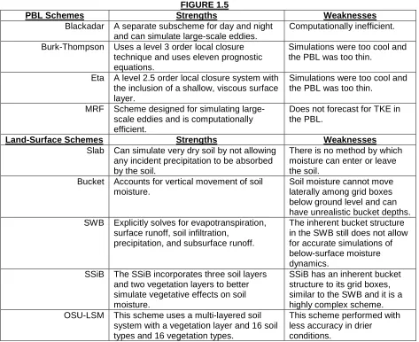
Bright and Mullen (2002) evaluated the performance of four PBL schemes (Blackadar, MRF, Eta, and Burk-Thompson) in the summer of 2000 for Arizona and New Mexico. Results from Bright and Mullen (2002) include the following: (1) Blackadar (BLK) and MRF simulated the PBL more accurately than the Eta or Burk- Thompson (BT) schemes, which were too cool, too moist and the PBL was too thin; (2) the thermodynamic qualities simulated by BLK and MRF were more accurate than the Eta or BT; and (3) the MM5 model coupled with MRF will be 15% faster than the MM5 coupled with the BLK.
FIGURE 1.5
PBL Schemes Strengths Weaknesses Blackadar A separate subscheme for day and night
and can simulate large-scale eddies.
Computationally inefficient. Burk-Thompson Uses a level 3 order local closure
technique and uses eleven prognostic equations.
Simulations were too cool and the PBL was too thin.
Eta A level 2.5 order local closure system with the inclusion of a shallow, viscous surface layer.
Simulations were too cool and the PBL was too thin.
MRF Scheme designed for simulating large-scale eddies and is computationally efficient.
Does not forecast for TKE in the PBL.
Land-Surface Schemes Strengths Weaknesses Slab Can simulate very dry soil by not allowing
any incident precipitation to be absorbed by the soil.
There is no method by which moisture can enter or leave the soil.
Bucket Accounts for vertical movement of soil moisture.
Soil moisture cannot move laterally among grid boxes below ground level and can have unrealistic bucket depths. SWB Explicitly solves for evapotranspiration,
surface runoff, soil infiltration, precipitation, and subsurface runoff.
The inherent bucket structure in the SWB still does not allow for accurate simulations of below-surface moisture dynamics.
SSiB The SSiB incorporates three soil layers and two vegetation layers to better simulate vegetative effects on soil moisture.
SSiB has an inherent bucket structure to its grid boxes, similar to the SWB and it is a highly complex scheme. OSU-LSM This scheme uses a multi-layered soil
system with a vegetation layer and 16 soil types and 16 vegetation types.
This scheme performed with less accuracy in drier conditions.
Figure 1.5: Relevant strengths and weaknesses in the four PBL schemes studied by Bright and Mullen (2002) and the five land-surface schemes as compared by Chen et al. (1996).
tested by Chen et al. (1996). The less complex MRF PBL scheme performed the best because it was able to simulate large-scale eddies that exist in the PBL (Bright and Mullen, 2002).
1.7. Thesis Organization
The goal of this thesis is to evaluate the MM5 model performance in forecasting near-surface parameters. This evaluation will be conducted on two fronts: (1) comparing the performance of the MM5 and Eta against observations and (2) comparing the performance of the MM5 with different land-surface schemes. Chapter 3 will detail the performance of the MM5 compared to the Eta and Chapter 4 will compare the results among the three land-surface schemes employed by the MM5. Chapters 5 through 7 focus on one model run (from 0000 UTC 7 December 2001) that was used as a sensitivity test. Chapter 5 describes the analyzed synoptic conditions from the forecast period. Chapter 6 compares the model runs from MM5 and Eta that initiated at 0000 UTC 7 December 2001 against the observations of temperature, dew point, and 1000-850 mb thickness. Chapter 7 evaluates the performance of the MM5 with three different soil moisture techniques in the
2.1. Observation Stations
Data were collected from the 0000 UTC run of the MM5 model (both the 45km and the 15km grids), and the 0000 UTC Eta model every day from 11
September 2001 through 12 December 2001. The standard 80-km (211 grid) of the Eta model was utilized in this study. To evaluate the performance of these two models in simulating the conditions of the lower troposphere, the model forecasts and observations for three parameters were recorded: (1) 2-meter temperature, (2) 2-meter dew point, and (3) 1000-850 mb thickness. The following sites were used in the original study: (1) Fayetteville, North Carolina, Regional Airport (KFAY); (2) Greenville, North Carolina (KPGV); (3) Raleigh-Durham, North Carolina,
International Airport (KRDU); (4) Rocky Mount-Wilson, North Carolina, Airport (KRWI); and (5) Southern Pines, North Carolina (KSOP) [See Figure 2.1 for a map of the sites used in the original study]. These five sites were chosen for three
specific reasons: (1) they were inside the fine 15km-grid of the MM5 model, (2) each site recorded hourly ASOS data of 2-meter temperature and 2-meter dew point, and (3) they were located near the WRAL-TV viewing area.
2.2. Types of Data Included
and 1200 UTC each day and interpolated to each site.
The gridded data forecasted by each model is interpolated to each observation site through an inverse distance relationship. The two grid points closest to an observation site are used in the interpolation. The square of the inverted distance is normalized and used as a coefficient to the value of temperature, dew point, or 1000-850 mb thickness.
2.3. Model configuration and physics
The inclusion of the results from the entire study period serve two purposes: (1) to evaluate how the two MM5 domains and the Eta model forecast 2-meter temperature, 2-meter dew point, and 1000-850 mb thickness compared to the observations, and (2) to evaluate how the different land-surface schemes used by the MM5 affected the forecast 2-meter temperature, 2-meter dew point, and 1000-850 mb thickness.
The Eta model was chosen as a control model because the model physics and horizontal grid spacing did not change during the test period from 11 September through 12 December. Also, the Eta is a widely-used numerical model produced by the National Centers for Environmental Prediction (NCEP) for short-term forecasting of near-surface temperature and dew point.
original data are nudged in order to dampen out the effects of gravity waves and to provide the most recent analysis of the initial fields.
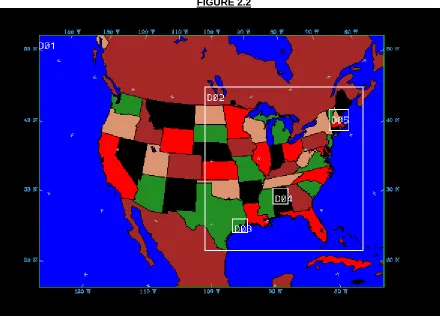
The MM5 model produces forecasts starting at 0000 UTC and 1200 UTC daily. The MM5 is a nested-grid model with a 45-km North American grid and a 15-km southeast regional grid, with a one-way interaction [See Figure 2.2 for a map of the nested MM5 grids]. The 45-km grid is initialized from the 40-km Eta 212 model analysis, and the 15-km regional grid is initialized from the 45-km analysis. The 45-
FIGURE 2.2
Figure 2.2: Nested grids of the SECMEP MM5 model. Domain D01 is the 45km North
km coarse domain utilizes a 96x132 horizontal grid, and the 15-km fine domain utilizes a 190x184 horizontal grid. Both domains of the MM5 have 31 vertical layers, with 100 mb as the top layer, and an average of twelve to fifteen vertical layers within the planetary boundary layer (PBL).
The MM5 model is currently configured with the Reisner-1 Mixed Phase cloud microphysics scheme, the RRTM/Dudhia-shortwave radiation scheme (Dudhia, 1989), the Kain-Fritsch deep convection scheme (Kain and Fritsch, 1990 and Kain and Fritsch, 1992), the MRF planetary boundary layer scheme (Hong and Pan, 1996), and the OSU-LSM (Mahrt and Pan, 1984; Mahrt and Ek, 1984; Pan and Mahrt, 1987).
2.4. Changes to the MM5 During the Study Period
University Land-Surface Model (OSU-LSM) developed by Mahrt and Pan (1984); Mahrt and Ek (1984); and Pan and Mahrt (1987). The OSU-LSM remained
integrated in the MM5 model until the end of the original study period (12 December 2001).
2.4.a. Soil Moisture Scaling Technique
As discussed in Chapter 1, the OSU-LSM resolves four soil layers, with the layer tops at 0.1 m, 0.3 m, 0.6 m, and 1.0 m, and modeling a total depth of 2 meters. The OSU-LSM resolves an initial amount of soil moisture in each layer based upon observations, then interpolating the point observations across the entire model grid. The scaled soil moisture technique arbitrarily increases or decreases the amount of initial soil moisture in each layer to more accurately reflect the actual amount of soil moisture. It is hoped that by producing a more accurate representation of initial soil moisture, the MM5 will produce a better representation of the diurnal cycle of
temperature, dew point, and 1000-850 mb thickness.
2.5. Numerical Methods Utilized
Two statistical measures of forecast accuracy were utilized in the comparison of the MM5 model output in the original study period: (1) mean absolute error (MAE) [Eqn. 1], hereafter referred to as the “error”, and (2) bias (B) [Eqn. 2].
Where f is an individual forecasted value, o is an individual observed value, n is the total number of data points, k is an individual data point, f is the average of all forecasted values, and o is the average of all the observations.
The bias is a difference of means, but the error is a sum of absolute
3. Model Comparison
3.1. Observed Weather Conditions from the Study Period
Figures 3.1 through 3.5 are time-series plots of forecasted and observed 2-meter temperature, 2-2-meter dew point, and 24-hour precipitation. Figures 3.1 and 3.2 are time series plots of observed and forecasted 2-meter temperature at F12 (1200 UTC Day 1) and F24 (0000 UTC Day 2). A recurrence of a maximum in the temperatures at both 1200 UTC (0700 LST) and 2400 UTC (1900 UTC) is detected every 6-8 days. The sharp drop in temperature after the peak temperature further supports the observation of periodic cold fronts passing through RDU every 6-8 days.
Figures 3.3 and 3.4 are time series plots of 2-meter dew point at 0700 LST and 1900 LST every day in the study period. A similar recurrence of maximum dew points every 6-8 days occur in the observations of dew point likely due to periodic cold fronts passing through RDU during the study period.
Figure 3.5 is a time series plot of 24-hour precipitation totals for each day in the study period. There was more than a trace of precipitation on only eight days out of the 93 days of the entire study period. These eight days coincided with the passage of the cold fronts as depicted in Figures 3.1 through 3.5. The days with rainfall of at least 0.05 inches occurred within 48 hours of a cold front passage.
3.2. Results from the Model Comparison
3.2.a. 2-meter Temperature
biases and errors include: (1) the Eta generally produces forecasts that have a smaller variance from run-to-run than those from either of the MM5 domains; (2) the Eta model forecasts the diurnal cycle more accurately than either MM5 domain; (3) there is no clear advantage in using the higher resolution of the Fine MM5 in place of the Coarse MM5; (4) both MM5 domains have a minimum in forecast errors during “diurnal transitions”; and (5) the rapid increases and decreases in the cold bias may be attributed to the formation and collapse of the mixed layer, when day shifts to night (or vice versa). The higher degree of success found in the Eta model forecasts may be attributed to either a more accurate land-surface or PBL scheme.
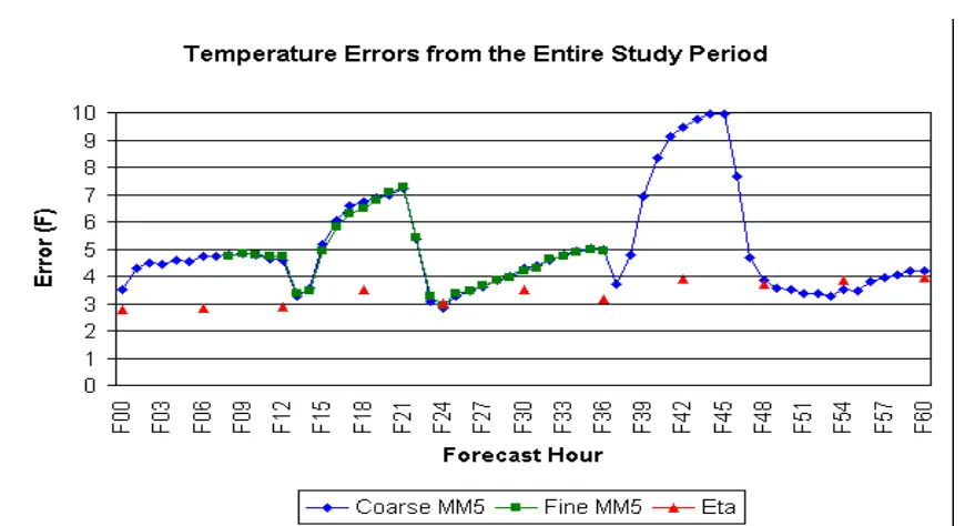
Figures 3.6 and 3.7 show average forecast biases (3.6) and errors (3.7), standard deviations, and variances. Not only are the forecast errors from the Eta model less than those from the MM5, the Eta model forecasts with less variance than the MM5 [see Figure 3.7]. At F42, the Coarse MM5 forecasts with the most error (9.5 °F) and with the highest variance (22.4 °F). At the same time, the Eta forecasts with a variance of 10.9 °F. F42 is also the most inaccurate time in all model runs. At all other times in the forecast period, the variances from the Eta forecasts were lower than those from the MM5.
FIGURE 3.6 FIGURE 3.7
TEMPERATURE BIASES TEMPERATURE ERRORS
COARSE MM5 FINE MM5 ETA COARSE MM5 FINE MM5 ETA
F
O
RCAS
T
HOUR M
E AN S T D. DEV . V ARI
ANCE ME
AN S T D. DEV . V ARI
ANCE ME
AN S T D. DEV . V ARI ANCE F O RCAS T
HOUR M
E AN S T D. DEV . V ARI
ANCE ME
AN S T D. DEV . V ARI
ANCE ME
AN S T D. DEV . V ARI ANCE
F00 2.1 2.6 6.7 1.3 1.9 3.5 F00 3.5 1.8 3.1 2.8 1.2 1.4
F06 3.7 3.8 14.2 -0.2 2.5 6.0 F06 4.7 3.0 8.8 2.8 1.2 1.5
F12 3.8 3.6 13.0 4.0 3.6 12.6 -0.9 3.0 9.1 F12 4.6 3.0 8.9 4.7 3.0 8.8 2.9 1.8 3.2 F18 -6.2 4.2 17.6 -5.4 4.0 15.7 -0.7 4.2 18.0 F18 6.7 3.1 9.6 6.5 3.0 8.7 3.5 2.5 6.4
F24 0.0 2.2 4.8 0.2 2.2 5.1 1.0 2.9 8.6 F24 2.8 0.9 0.8 2.9 1.1 1.1 3.0 1.8 3.2
F30 3.3 3.1 9.8 3.4 2.8 8.0 1.8 3.1 9.6 F30 4.3 2.3 5.1 4.2 2.3 5.1 3.5 2.0 3.9
F36 4.1 3.7 13.6 4.4 3.3 10.8 0.7 3.2 10.5 F36 5.0 2.7 7.4 4.9 2.7 7.1 3.2 1.5 2.2
F42 -8.9 5.8 33.9 0.0 5.1 26.2 F42 9.5 4.7 22.4 3.9 3.3 10.9
F48 -2.5 3.4 11.5 0.8 3.7 13.9 F48 3.8 2.3 5.4 3.7 1.9 3.6
F54 1.0 3.2 10.3 0.9 4.2 17.7 F54 3.5 1.9 3.7 3.8 2.4 5.7
F60 1.9 3.9 15.3 0.2 4.2 18.0 F60 4.2 2.2 4.8 3.9 2.2 4.8
Figures 3.6, 3.7: Mean, Standard Deviation, and Variance from the entire study period for the Coarse MM5, Fine MM5, and Eta models. These tables show data of biases (2.7) and errors (2.8) in 2-meter temperature.
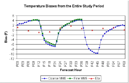
FIGURE 3.8
Figure 3.8: Average biases (in °°°°F) for 2-meter temperature for the Coarse MM5, Fine MM5, and
FIGURE 3.9
Figure 3.9: Average errors (in °°°°F) for 2-meter temperature for the Coarse MM5, Fine MM5, and
Eta model at each forecast hour.
hour from F00 through F48. Only at F24 and after F48 were the forecast accuracies from the Coarse MM5 and Eta comparable.
The increased horizontal resolution of the Fine MM5 did not forecast 2-meter temperature significantly better than the Coarse MM5. Figure 3.8 plots the study-averaged forecast bias from both MM5 domains. The biases from the Fine MM5 and Coarse MM5 overlap at all times except from F15 through F21, where the Fine MM5 forecasted with a 0.5 °F - 1.0 °F improvement in the cold bias. The warm bias was similar in both domains of the MM5. The forecasted errors (Figure 3.9) overlap at every forecast hour.
the diurnal cycle switches from night to day. F24 occurs at 0000 UTC (1900 LST), when day transitions to night. The Coarse MM5 forecast errors at these times were 3.5 °F, 3.0 °F, and 3.8 °F at F13, F24, F37, respectively.
The cold bias (Figure 3.8) that develops in the Coarse MM5 forecasts forms rapidly in the first four hours of daylight, and disappears rapidly in the three hours around sunset. Rapid changes in the bias also occur in the evening [See Figure 3.8]. The disappearance of the cold bias in the evening is less sudden than its appearance in the morning. The appearance and disappearance of the cold bias in the MM5 forecasts is well timed with the formation and collapse of the turbulent mixed layer. This observation suggests that a PBL scheme may have some importance in the forecasts of 2-meter temperature.
3.2.b. 2-meter Dew Point
moisture from the ground. It is expected that on a day with a strong, or deep, mixed layer, that the highest dew point should be observed in the few hours after sunrise. The lowest dew point should occur either a few hours after sunset, or just before sunrise, if the temperature approaches the dew point.
A few observations can be drawn from a study of the three models’
forecasting skill of 2-meter dew point: (1) the variance in the MM5 forecast bias is more dependent on diurnal factors, where the Eta is more dependent on increased forecast time; (2) variance in forecast error from all models is dependent on diurnal factors; (3) although all models forecasted dew point with a positive bias, the MM5 forecasts combined this with a diurnal pattern; and (4) the Eta model forecasts 2-meter dew point with less error and a more neutral bias than the forecasts from the Coarse MM5.
FIGURE 3.10 FIGURE 3.11
DEW POINT BIASES DEW POINT ERRORS
COARSE MM5 FINE MM5 ETA COARSE MM5 FINE MM5 ETA
F
O
RCAS
T
HOUR M
E AN S T D. DEV . V ARI
ANCE ME
AN S T D. DEV . V ARI
ANCE ME
AN S T D. DEV . V ARI ANCE F O RCAS T
HOUR M
E AN S T D. DEV . V ARI
ANCE ME
AN S T D. DEV . V ARI
ANCE ME
AN S T D. DEV . V ARI ANCE
F00 3.5 3.2 10.4 -0.3 2.8 8.1 F00 4.2 2.4 5.8 3.0 1.6 2.6
F06 3.9 2.2 5.0 0.1 2.4 5.7 F06 4.2 1.8 3.4 2.8 1.2 1.4
F12 4.7 2.5 6.5 5.2 2.6 6.9 -0.3 3.0 9.1 F12 4.9 2.3 5.4 5.3 2.5 6.4 2.8 1.6 2.6
F18 4.7 4.3 18.3 5.4 4.5 19.9 3.0 3.1 9.6 F18 5.2 3.8 14.4 5.6 4.2 17.6 3.9 2.2 4.8
F24 4.5 3.3 10.8 5.3 3.6 13.1 1.9 3.4 11.2 F24 4.7 3.1 9.5 5.4 3.5 12.1 3.7 1.9 3.5
F30 4.7 3.1 9.8 5.1 3.2 10.0 1.8 3.4 11.9 F30 5.0 2.8 7.7 5.3 2.9 8.6 3.8 1.9 3.5
F36 5.2 3.8 14.2 5.5 3.4 11.7 1.1 3.6 12.8 F36 5.7 3.1 9.5 5.8 3.0 8.8 3.4 1.7 2.9
F42 3.2 4.9 24.0 3.0 3.5 12.4 F42 4.9 3.3 11.2 4.3 2.4 5.6
F48 2.8 4.0 16.0 1.6 3.2 10.2 F48 4.3 2.5 6.4 3.7 1.7 2.8
F54 3.3 4.3 18.6 2.0 4.3 18.5 F54 4.8 3.0 9.0 3.9 2.6 6.7
F60 3.3 4.6 20.7 1.1 5.0 24.7 F60 5.2 2.6 6.9 4.4 2.6 6.8
Figures 3.10, 3.11: Same as Figures 3.6 and 3.7, except data is from the forecast biases (3.10) and errors (3.11) of 2-meter dew point.
Figure 3.12 displays the average dew point forecast bias from each of the three models (Coarse MM5, Fine MM5, and Eta). It can be noted that all models display a positive bias (especially after F12); moreover, there seems to be a diurnal pattern superimposed over the consistent positive dew point bias. The lowest positive bias occurs near F15 and F39 (1000 LST), when the diurnal pattern completes the shift from night to day and when the mixed layer becomes well established. Secondary minima occur near F24 and F48 (1900 LST) when the mixed layer collapses at the end of the day.
FIGURE 3.12
Figure 3.12: Average biases (in °°°°F) for 2-meter dew point for the Coarse MM5, Fine MM5, and
Eta model at each forecast hour.
FIGURE 3.13
Figure 3.13: Average errors (in °°°°F) for 2-meter dew point for the Coarse MM5, Fine MM5, and
An inaccurate simulation of soil moisture, and the fluxes of moisture from soil to air, can lead to an inaccurate simulation of near-surface dew point. Some
incoming solar radiation that reaches the ground goes to evaporation. The soil moisture then evaporates and adds to the amount of water vapor in the air (i.e. the dew point increases). If a model’s land-surface scheme incorrectly simulates the amount of soil moisture, or the ability of the soil to evaporate moisture, then the model may produce inaccurate forecasts of dew point. In the study described above, the MM5 has a consistent positive dew point bias that reaches a maximum during the warmest part of the day. This suggests that the MM5 is evaporating too much water into the lower troposphere, which leads to an incorrectly high forecast for dew point. This kind of dew point forecast error can also lead to a cold bias in the temperature forecast because the model attempts to use incoming solar
radiation to evaporate the water. The end result is a cooler forecast of temperature than was observed (i.e. a daytime cold bias). The surplus water vapor has a reverse effect at night, when the model overestimates the outgoing radiation being absorbed by water vapor. The absorption of outgoing radiation leads to an increased
temperature forecast at night (i.e. a nighttime warm bias).
The planetary boundary layer is also affected by a change in surface layer moisture. The mixed layer depth is dependent on relative humidity, so a decrease in the surface dew point will cool the surface layer, which acts to reduce the height of the mixed layer. Stull (1988) noted that mixed layer growth was tied with the solar heating reaching the ground. Since the amount of solar radiation working to
low-level water vapor, higher near-surface dew points will lead to a lower PBL height. A model’s PBL scheme has an influence here as well. An inaccurate simulation of the PBL may lead to an inaccurate forecast of surface temperature or dew point.
3.2.c. 1000-850 mb Thickness
We wish to expand our analysis beyond a single level (2 meters). The
vertical interpolation to obtain 2-meter values is sensitive, and a layer average offers a more useful calculation. To infer a sense of an average layer temperature near the surface, the forecasts and observations of 1000-850 mb thickness were used. According to the hypsometric equation, the virtual temperature of a layer in the troposphere can be inferred by determining the height between two pressure levels.
) ln( 2 1 P P T a z = • v• ∆
The equation above is the hypsometric equation, where∆zis the thickness,
K m g
Rd
a= / =29.3 / , Tv is virtual temperature, and P1 and P2 are two pressure
levels. By evaluating the models’ performance in forecasting 1000-850 mb
thickness, one can gain an understanding of the forecasting ability of the MM5 and Eta in resolving the boundary layer temperature.
MM5 in the forecasting of 1000-850 mb thickness; and (3) the MM5 has a severe cold bias in 1000-850 mb thickness that forms after F09.
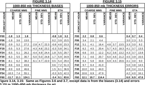
Figure 3.14 shows the mean, standard deviation, and variance of 1000-850 mb thickness forecasts from the Coarse MM5, Fine MM5, and Eta model domains. Figure 3.15 shows similar data as Figure 3.7, but for the forecast errors of 1000-850 mb thickness. The variances in 1000-850 mb thickness forecasting at F00 are the smallest of any variance at any time for any parameter. At F60, the variance in the Coarse MM5 forecast errors was 114.4 m, but 47.6 m for the Eta forecast errors. This suggests that the MM5 has very little accuracy in forecasting 1000-850 mb thickness, especially after F36.
Figures 3.16 and 3.17 plot the average forecast bias (3.16) and error (3.17) of 1000-850 mb thickness from all three models. In the bias and error patterns
FIGURE 3.14 FIGURE 3.15
1000-850 mb THICKNESS BIASES 1000-850 mb THICKNESS ERRORS
COARSE MM5 FINE MM5 ETA COARSE MM5 FINE MM5 ETA
F
O
RCAS
T
HOUR M
E AN S T D. DEV . V ARI
ANCE ME
AN S T D. DEV . V ARI
ANCE ME
AN S T D. DEV . V ARI ANCE F O RCAS T
HOUR M
E AN S T D. DEV . V ARI
ANCE ME
AN S T D. DEV . V ARI
ANCE ME
AN S T D. DEV . V ARI ANCE
F00 -1.8 1.3 1.8 -0.8 1.8 3.2 F00 2.2 0.8 0.6 0.4 0.7 0.4
F06 -1.8 3.6 13.0 0.2 3.9 15.5 F06 3.4 2.1 4.4 3.0 2.3 5.3
F12 -3.9 5.2 27.2 -2.8 4.7 22.3 -0.8 4.8 23.3 F12 5.1 4.1 16.4 4.8 3.7 13.5 3.3 3.0 9.2
F18 -5.5 5.3 27.6 -4.3 4.8 23.2 -0.3 5.8 34.1 F18 6.2 4.5 20.4 5.7 4.3 18.3 4.1 3.7 13.5
F24 -5.5 5.1 26.2 -4.4 4.9 24.4 1.8 5.5 29.7 F24 6.6 3.5 12.2 6.2 3.6 13.2 4.3 3.7 13.9
F30 -6.3 5.5 30.7 -5.0 5.0 24.8 1.7 5.9 34.9 F30 7.1 4.6 20.7 6.0 4.6 21.2 4.5 3.9 15.5
F36 -8.1 6.2 38.2 -6.1 4.7 22.0 0.5 5.4 29.4 F36 8.4 5.8 33.8 6.9 4.5 20.6 4.1 3.0 9.0
F42 -9.6 6.6 43.6 0.6 7.2 51.3 F42 9.7 6.4 41.0 5.0 3.8 14.5
F48 -9.9 6.8 46.6 1.5 6.1 36.9 F48 10.0 6.6 44.0 4.9 3.4 11.3
F54 -10.3 7.4 55.1 -0.3 6.5 42.3 F54 10.6 6.9 47.9 4.2 4.0 16.1
F60 -11.7 11.1 124.1 -3.4 9.1 83.6 F60 12.1 10.7 114.4 6.0 6.9 47.6