78: 6-13 (2016) 37–44 | www.jurnalteknologi.utm.my | eISSN 2180–3722 |
Jurnal
Teknologi
Full Paper
ROBUST
HOVERING
CONTROLLER
FOR
UNCERTAIN
MULTIROTOR
MICRO
AERIAL
VEHICLES
(MAVS)
IN
GPS-DENIED
ENVIRONMENTS: IMAGE-BASED
Dafizal Derawi
a,b, Nurul Dayana Salim
a,b, Hairi Zamzuri
a,*, Mohd Azizi
Abdul Rahman
a, Kenzo Nonami
ca
Malaysia-Japan International Institute of Technology, Universiti
Teknologi Malaysia, Kuala Lumpur, Malaysia
b
Mechatronic Systems Laboratory, Robotic Systems Enterprise,
Melaka, Malaysia
c
Faculty of Engineering, Chiba University, Chiba, Japan
Article history
Received 1 November 2015 Received in revised form
21 March 2016 Accepted 23 March 2016
*Corresponding author
[email protected]
Graphical abstract
Abstract
This paper proposes an image-based robust hovering controller for multirotor micro aerial vehicles (MAVs) in GPS-denied environments. The proposed controller is robust against the effects of multiple uncertainties in angular dynamics of vehicle which contain external disturbances, nonlinear dynamics, coupling, and parametric uncertainties. Based on visual features extracted from the image, the proposed controller is capable of controlling the pose (position and orientation) of the multirotor relative to the fixed-target. The proposed controller scheme consists of two parts: a spherical image-based visual servoing (IBVS) and a robust flight controller for velocity and attitude control loops. A robust compensator based on a second order robust filter is utilized in the robust flight control design to improve the robustness of the multirotor when subject to multiple uncertainties. Compared to other methods, the proposed method is robust against multiple uncertainties and does not need to keep the features in the field of view. The simulation results prove the effectiveness and robustness of the proposed controller.
Keywords: Image-based; robust control; hovering; multirotor micro aerial vehicles
© 2016 Penerbit UTM Press. All rights reserved
1.0 INTRODUCTION
Multirotor micro aerial vehicles (MAVs) are widely used for many monitoring and surveillance tasks, in both indoor and outdoor environments. They are highly manoeuvrable, able to fly at low altitude, and are easier to control than traditional helicopter. Quadrotor platform has become the universal testbed for aerial robotic researches and a standard platform for multirotor MAV. It consists of four rotors attached to a rigid body frame and has the ability to do vertical take-off and landing (VTOL).
Over the last decades, different advanced control schemes have been developed for aerial vehicles.
visual servo (IBVS), the error is determined in the 2D image plane by controlling the task directly from the image plane (no pose estimation of the target). By defining the control task directly within the image coordinate space, the controller is inherently robust to camera calibration and alleviates the requirement for a 3D model of the target [1].
Position control with respect to fixed targets by using image features is a popular application for helicopters capable of hovering or near hovering flight [2]-[4]. However, their methods require a very accurate model of the target and is very difficult to obtain when it deals with dynamics system. For observing fixed targets from a fixed-wing aircraft, hovering task is not possible since it has to maintain the forward velocity for lifting and usually, they will do circular orbits using IBVS technique [5]-[7]. Automated landing of fixed-wing aircraft has also been a popular application of IBVS control, utilizing a desired view of runway features to achieve control during each phase of landing [7]-[11]. However, the effects of multiple uncertainties in vehicle dynamics were not addressed in previous studies. In addition, previous research which relied on IBVS has difficulty in keeping the target features in field of view.
In this paper, the proposed image-based robust controller is capable of controlling the pose (position and orientation) of the multirotor MAV with respect to fixed-target points without the GPS and it relies on visual features extracted from the image only. The proposed controller consists of two parts: the spherical image-based visual servoing (IBVS) controller and the robust flight controller based on robust compensating technique [12]. The camera model is an “eye-in-hand” type configuration, where a downward facing camera is attached to the centre of the airframe of the multirotor MAV. The dynamic of the system is modelled to determine the dynamic responses of the camera signals based on general assumptions about the structure of the environment. The simulation results prove the effectiveness and robustness of the proposed controller and show high potential for practical applications.
This paper is different compared to previous works since it proposes an image-based robust hovering control for multirotor MAVs which considers the influence of multiple uncertainties in angular dynamics of vehicle and utilizes a new method of spherical imaging technique for camera model introduced in [13]. As a result, multirotor MAVs are robust against uncertainties such as disturbances, nonlinear dynamics, coupling, and parametric uncertainties and does not require keeping target features in the field of view.
The rest of this paper is arranged as follows. Section 2 describes the system overview. Section 3 presents the proposed image-based robust hovering control scheme for the multirotor MAV. Section 4 presents the simulation results and finally, Section 5 summarizes this paper and provides suggestion for future research.
2.0 SYSTEM
2.1 Model of Multirotor Micro Aerial Vehicle
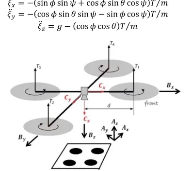
As mentioned earlier, the quadrotor platform has become a universal testbed for aerial robotic researches and the standard platform of multirotor MAVs. Thus, the rigid body dynamics of the quadrotor is described in this section. The quadrotor consists of four rotors attached to a body frame as shown in Figure 1.
Let us define {𝐴} = {𝐴𝑥, 𝐴𝑦, 𝐴𝑧} as an inertial frame,
{𝐵} = {𝐵𝑥, 𝐵𝑦, 𝐵𝑧} denote a body-fixed frame for the quadrotor airframe, {𝐶} = {𝐶𝑥, 𝐶𝑦, 𝐶𝑧} denote a camera-fixed frame. As can be seen, the camera and body-fixed frames have their positive z-axis downward following the standard aerospace convention. The camera is fixed and centred at the centre of gravity (CoG) of {𝐵}. Let us denote 𝜉 = (𝜉𝑥 𝜉𝑦 𝜉𝑧)𝑇∈ {𝐴} as the position of the origin of the body-fixed frame {𝐵}
with respect to inertial frame {𝐴} and 𝜂 = (𝜙 𝜃 𝜓)𝑇∈
{𝐵} as the attitude vector of roll 𝜙, pitch 𝜃, and yaw 𝜓
angles. The rigid body dynamics model can be derived by the Euler-Lagrange approach as [14]
𝜉̈𝑥= −(sin 𝜙 sin 𝜓 + cos 𝜙 sin 𝜃 cos 𝜓)𝑇 𝑚⁄
𝜉̈𝑦= −(cos 𝜙 sin 𝜃 sin 𝜓 − sin 𝜙 cos 𝜓)𝑇 𝑚⁄
𝜉̈𝑧= 𝑔 − (cos 𝜙 cos 𝜃)𝑇 𝑚⁄
(1)
Figure 1 Notation for the quadrotor in hovering control task
𝜙̈ = 𝐼𝜙−1𝐶𝜙(𝜂, 𝜂̇)𝜂̇ + 𝐼𝜙−1(𝜏𝜙+ 𝑤𝜙)
𝜃̈ = 𝐼𝜃−1𝐶𝜃(𝜂, 𝜂̇)𝜂̇ + 𝐼𝜃−1(𝜏𝜃+ 𝑤𝜃)
𝜓̈ = 𝐼𝜓−1𝐶𝜓(𝜂, 𝜂̇)𝜂̇ + 𝐼𝜓−1(𝜏𝜓+ 𝑤𝜓)
(2)
where 𝐶𝑖(𝜂, 𝜂̇)(𝑖 = 𝜙, 𝜃, 𝜓) is the Coriolis term [14], 𝑇 is the total thrust force, 𝑚 is the total mass of vehicle, 𝑔 is the gravity constant, 𝜏𝑖 (𝑖 = 𝜙, 𝜃, 𝜓) is the torque applied to the airframe by aerodynamics of rotors, 𝑤𝑖(𝑖 = 𝜙, 𝜃, 𝜓) is the external disturbance, and 𝐼𝑖 (𝑖 = 𝜙, 𝜃, 𝜓) is the moments of inertia. Actually, (1) and (2) describe the translational and rotational motions of the vehicle, respectively.
The thrust force 𝑇𝑖 (𝑖 = 1,2, 3, 4) is produced by single rotor in the air and can be modelled as [15]
𝑇𝑖= 𝑏𝜔𝑖2 (3)
𝑇 = ∑ 𝑇𝑖 4
𝑖=1
(4)
The torque 𝜏𝑖 (𝑖 = 𝜙, 𝜃, 𝜓) about each axis of body frame could be written as
𝜏𝜙= 𝑑(𝑇4− 𝑇2)
𝜏𝜃= 𝑑(𝑇1− 𝑇3)
𝜏𝜓= 𝑘𝑓𝑚(𝑇1− 𝑇2+ 𝑇3− 𝑇4)
(5)
where 𝑑 is the distance between the centre of mass and the rotor, 𝑘𝑓𝑚 denotes the positive force-to-torque scaling factor in aerodynamics of rotor.
From (4), the control input of thrust 𝑢𝑇 could be defined as
𝑢𝑇= 𝜔12+ 𝜔22+ 𝜔32+ 𝜔42 (6)
From (5), the attitude control input for roll 𝑢𝜙, pitch 𝑢𝜃, and yaw 𝑢𝜓 could be defined as
𝑢𝜙= 𝜔42− 𝜔22
𝑢𝜃= 𝜔12− 𝜔32
𝑢𝜓= 𝜔12− 𝜔22+ 𝜔32− 𝜔42
(7)
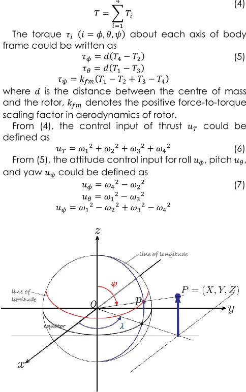
Figure 2 The coordinate system. 𝑃 is mapped to 𝑝 on the
sphere represented by colatitude 𝜑 and longitude 𝜆.
From (5) and (7), the attitude control input for roll, pitch, and yaw angles are proportional to torque, such that 𝜏𝑖= 𝑎𝑖1𝑢𝑖 where 𝑎𝜙1= 𝑑𝑏, 𝑎𝜃1= 𝑑𝑏, and 𝑎𝜓1= 𝑘𝑓𝑚𝑏. In practice, the control inputs will be distributed to each motor by using a power distribution board and thus, the control inputs can be controlled directly to control the motions of the vehicle.
Let us define the vehicle parameter constant 𝑎𝑖=
𝐼𝑖−1𝑎𝑖1 (𝑖 = 𝜙, 𝜃, 𝜓) and it consists of nominal 𝑁 and uncertain Δ values, such that
𝑎𝑖= 𝑎𝑖𝑁+ 𝑎𝑖Δ, 𝑖 = 𝜙, 𝜃, 𝜓
Assumption 1: The uncertain part 𝑎𝑖Δ are bounded. The nominal part 𝑎𝑖𝑁> 0 and satisfies |𝑎𝑖𝑁− 𝑎𝑖| < 𝑎𝑖𝑁. Let us define the positive constant 𝜌𝑖 (𝑖 = 𝜙, 𝜃, 𝜓) as 𝜌𝑖=
|𝑎𝑖𝑁− 𝑎𝑖| 𝑎⁄ 𝑖𝑁. Therefore, 𝜌𝑖 satisfy that 0 ≤ 𝜌𝑖< 1. Assumption 2: The total upward thrust is bounded with 𝑇 ≥ 𝛿𝑇 where 𝛿𝑇> 0.
Assumption 3: The pitch and roll angles satisfy that 𝜃 ∈ (−𝜋 2⁄ + 𝛿𝜃, 𝜋 2⁄ − 𝛿𝜃) and 𝜙 ∈ (−𝜋 2⁄ + 𝛿𝜙, 𝜋 2⁄ − 𝛿𝜙) where 𝛿𝑖> 0 (𝑖 = 𝜃, 𝜙).
Assumption 4: The external disturbance 𝑤𝑖(𝑖 = 𝜙, 𝜃, 𝜓) is bounded.
Assumption 5: The attitude angles have the desired reference signal as 𝑖𝑑 (𝑖 = 𝜙, 𝜃, 𝜓). The reference signals and their derivatives 𝑖𝑑(𝑘) (𝑖 = 𝜃, 𝜙, 𝜓; 𝑘 = 0,1,2) are piecewise uniformly bounded.
Assumption 6: The effects of uncertainties in translational motion (1) are very small in hovering conditions. Thus, the effects of uncertainties in (1) can be ignored. If the angular dynamics (rotational motion) of the multirotor MAV is robust, then the whole flight controller is robust in hovering conditions.
2.2 Image Jacobian for Spherical Camera
The catadioptric camera and fisheye lens camera are popular types of non-perspective cameras in literature. Because of that, many different projection models and image Jacobians were developed in literature. One alternative is that the features from any type of camera can be projected to sphere as shown in Figure 2.
The image Jacobian is derived using the similar method that has been used for perspective camera. Let us consider the camera is moving with velocity
𝑣 = (𝑣𝑥, 𝑣𝑦, 𝑣𝑧)𝑇 and angular velocity 𝜔 = (𝜔𝑥, 𝜔𝑦, 𝜔𝑧)𝑇 and it is observing a world point 𝑃 in the world frame.
𝑃 = (𝑋, 𝑌, 𝑍) denotes the point with camera relative coordinates and the velocity of the point relative to the camera frame can be described as
𝑃̇ = −𝜔 × 𝑃 − 𝑣 (8)
From (8), it can be derived as
𝑋̇ = 𝑌𝜔𝑧− 𝑍𝜔𝑦− 𝑣𝑥
𝑌̇ = 𝑍𝜔𝑥− 𝑋𝜔𝑧− 𝑣𝑦
𝑍̇ = 𝑋𝜔𝑦− 𝑌𝜔𝑥− 𝑣𝑧
(9)
As can be seen in Figure 2, 𝑃 can be projected to point 𝑝 = (𝑥, 𝑦, 𝑧) on the sphere’s surface centred at the origin
𝑥 =𝑋
𝑅, 𝑦 =
𝑌
𝑅, 𝑧 =
𝑍 𝑅
(10)
where 𝑅 is the distance between the world point and camera origin with 𝑅 = √(𝑋2+ 𝑌2+ 𝑍2)
The spherical points satisfy that 𝑥2+ 𝑦2+ 𝑧2= 1 where one of the Cartesian coordinates is redundant. The angle of colatitude 𝜑 is defined by using minimal spherical coordinate system as shown in the following equation
𝜑 = sin−1𝑟 , 𝜑 ∈ [0, 𝜋) (11)
where 𝑟 = √𝑥2+ 𝑦2. The azimuth angle (longitude) is
𝜆 = tan−1𝑦
𝑥, 𝜆 ∈ [−𝜋, 𝜋) (12)
The Cartesian coordinates for the point feature 𝑝 = (𝜑, 𝜆) are
𝑥 = 𝑟 cos 𝜆 , 𝑦 = 𝑟 sin 𝜆 , 𝑧 = 𝑐𝑜𝑠𝜑 (13)
where 𝑟 = sin 𝜑. From (9)-(13), the following equation can be obtained
𝑋 = 𝑅 sin 𝜑 𝑐𝑜𝑠𝜆 𝑌 = 𝑅 sin 𝜑 sin 𝜆
𝑍 = 𝑅 cos 𝜑
(14)
(𝜑̇ 𝜆̇) = 𝐽(𝜑, 𝜆, 𝑅) ( 𝑣𝑥 𝑣𝑦 𝑣𝑧 𝜔𝑥 𝜔𝑦 𝜔𝑧) (15)
where the image feature Jacobian 𝐽(𝜑, 𝜆, 𝑅) is
𝐽 = ( −𝑐𝜆𝑐𝜑 𝑅 − 𝑠𝜆𝑐𝜑 𝑅 𝑠𝜑
𝑅 𝑠𝜆 −𝑐𝜆 0
𝑠𝜆 𝑅𝑠𝜑 − 𝑐𝜆 𝑅𝑠𝜑 0 𝑐𝜆𝑐𝜑 𝑠𝜑 𝑠𝜆𝑐𝜑
𝑠𝜑 −1)
(16)
where c and s denote cosine and sine, respectively.
3.0 ROBUST HOVERING CONTROLLER:
IMAGE-BASED
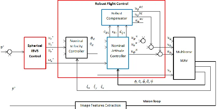
In this section, the task in robust hovering control is to control the pose of the multirotor MAV in hovering conditions relative to fixed targets (points) under the effects of uncertainties in the angular dynamics of vehicle by using visual features extracted from the image. The proposed control method does not require the state estimation of the target in Cartesian space and represents the task in terms of image error. The proposed method is particularly effective in situations where state estimation is difficult (e.g. GPS-denied environment). The overall proposed control deign is illustrated in Fig. 3.
Compared to the standard multirotor MAV control system:
1. The position errors for 𝜉𝑖 (𝑖 = 𝑥, 𝑦) in the proposed control design is given in the camera frame {𝐶}
(same with body-fixed frame {𝐵}), rather than inertial frame {𝐴}.
2. The horizontal position 𝜉𝑖(𝑖 = 𝑥, 𝑦), altitude 𝜉𝑧, and yaw angle 𝜓 loops are no longer required in the proposed controller since the spherical IBVS controller generates the required velocities for multirotor motions.
3.1 Spherical IBVS Control
The normal step of computing a 2 × 6 Jacobian in (16) for each 𝑁 feature points will result in
𝑣 = ( 𝐽1 ⋮ 𝐽𝑁 ) −1 ( 𝜑̇1 𝜆̇1 ⋮ 𝜑̇𝑁 𝜆̇𝑁) (17)
For 𝑁 > 3 the camera motion can be solved by using
the pseudo-inverse
𝑣 = 𝐽+𝑝̇∗ (18)
where 𝑝̇∗ denotes the desired velocity of the feature points in the 𝜆𝜑 -space. The solution that reduces the norm of the feature velocity error is obtained by pseudo-inverse. Then, the point velocity is computed by a proportional controller as
𝑝̇∗= 𝛼(𝑝∗− 𝑝) (19)
where 𝑝 is the current feature point in 𝜆𝜑 -space, 𝑝∗ is the desired value of the feature point, and 𝛼 denotes a gain which satisfies 𝛼 > 0.
As mentioned earlier, the camera frame {𝐶} is attached to the centre of the body frame {𝐵} and has similar positive direction of each axis. Therefore, the velocity of the camera is the same as the velocity of the multirotor MAV and thus, (17) can be written as
𝑣𝑑= 𝛼 ( 𝐽1 ⋮ 𝐽𝑁 ) +
(𝑝∗− 𝑝) (20)
𝑣𝑑= (𝑣𝑥∗ 𝑣𝑦∗ 𝑣𝑧∗ 𝜔𝑧∗)𝑇 is the desired velocity of the multirotor MAV. It will be the reference signal of the robust flight control system. 𝜔𝑥∗ and 𝜔𝑦∗ are not needed in the robust flight control system since roll and pitch subsystems are controlled directly based on desired roll
𝜙𝑑 and pitch 𝜃𝑑 angles.
3.2 Robust Flight Control
The velocity control loop looks at the desired velocity of rigid body (𝑣𝑥∗, 𝑣𝑦∗, 𝑣𝑧∗) produced by spherical IBVS control and compares that to the actual velocity of the multirotor MAV (𝜉̇𝑥 𝜉̇𝑦 𝜉̇𝑧). In practice, the actual velocity can be estimated by using a commercial inertial navigation system or an observer. The desired roll
𝜙𝑑 and pitch 𝜃𝑑 angles are generated by the nominal velocity controller a
𝜙𝑑= 𝐾1𝜙(𝑣𝑦∗− 𝐾2𝜙𝜉̇𝑦) (21)
𝜃𝑑= 𝐾1𝜃(𝑣𝑥∗− 𝐾2𝜃𝜉̇𝑥) (22) The altitude of the multirotor MAV 𝜉𝑧 is controlled by
𝑢𝑇= 𝐾1𝑇(𝑣𝑧∗− 𝐾2𝑇𝜉̇𝑧) + 𝜔0 (23)
where 𝐾1𝑖 and 𝐾2𝑖 with 𝑖 = (𝜙, 𝜃, 𝑇) are constant gains. 𝜔0 is the minimum rotor speed needed to produce a thrust equal to the weight of the aerial robot, that satisfies
𝜔0= √𝑚𝑔 4𝑏⁄ .
For attitude control loop, let us define an angular error vector as 𝑒𝑖= (𝑒𝑖1 𝑒𝑖2 𝑒𝑖3)𝑇 (𝑖 = 𝜙, 𝜃, 𝜓), where 𝑒𝑖1=
𝑖𝑑− 𝑖, 𝑒𝑖2= 𝑒̇𝑖1, and 𝑒̇𝑖3= 𝑒𝑖1.
Based on (2), let us define the error dynamical equations as
𝑒̇𝑖= 𝐴𝑖𝑒𝑖+ 𝐵𝑖(𝑢𝑖+ 𝑞𝑖), 𝑖 = 𝜙, 𝜃, 𝜓 (24) Where
𝐴𝑖= [
0 1 0 0 0 0
1 0 0], 𝐵𝑖= [ 0 𝑎𝑖𝑁
0 ]
and 𝑞𝑖 (𝑖 = 𝜙, 𝜃, 𝜓) is the multiple uncertainties in angular dynamics of vehicle which consists of external disturbances, nonlinear dynamics, coupling, and parametric uncertainties with the following equation
𝑞𝑖=
𝐼𝑖−1𝐶𝑖(𝜂, 𝜂̇)𝜂̇ + 𝑎𝑖Δ𝑢𝑖+ 𝐼𝑖−1𝑤𝑖− 𝑟̈𝑖
𝑎𝑖𝑁
(25)
The attitude controller design for roll, pitch, and yaw subsystems contain a nominal linear controller and robust compensator. As can be seen in Figure 3, the attitude control input 𝑢𝑖 (𝑖 = 𝜙, 𝜃, 𝜓) is
𝑢𝑖= 𝑢𝑖𝑁+ 𝑢𝑖𝑅𝐶 (26)
Figure 3 The overall block diagram of the proposed image-based robust hovering control of multirotor MAVs.
The nominal controller is designed based on proportional and derivative controllers to generate the nominal control input 𝑢𝑖𝑁(𝑖 = 𝜙, 𝜃)
𝑢𝜙𝑁= 𝐾𝜙𝑃(𝜙𝑑− 𝜙) + 𝐾𝜙𝐷(𝜙̇𝑑− 𝜙̇) (27)
𝑢𝜃𝑁= 𝐾𝜃𝑃(𝜃𝑑− 𝜃) + 𝐾𝜃𝐷(𝜃̇𝑑− 𝜃̇) (28) The terms 𝜙̇𝑑 and 𝜃̇𝑑 are commonly ignored since it is typically small. The gains 𝐾𝑖𝑃 and 𝐾𝑖𝐷 (𝑖 = 𝜙, 𝜃) are determined by classical method based on an approximation of dynamic model and can be tuned to achieve excellent tracking performance of the nominal system.
The nominal control input for yaw subsystem 𝑢𝜓𝑁 is generated by
𝑢𝜓𝑁= 𝐾1𝜓(𝜔𝑧∗− 𝐾2𝜓𝜓̇) (29) where 𝐾1𝜓 and 𝐾2𝜓 are constant gains. The actual angular rate along 𝐵𝑧 axis 𝜓̇ can be obtained by gyroscopes.
The robust compensator is introduced to reduce the effects of the multiple uncertainties 𝑞𝑖 (𝑖 = 𝜙, 𝜃, 𝜓) in angular dynamics by computing the robust compensating signal as
𝑢𝑖𝑅𝐶(𝑠) = −𝐹𝑖(𝑠)𝑞𝑖(𝑠), 𝑖 = 𝜙, 𝜃, 𝜓 (30) where 𝑠 is the Laplace operator and 𝐹𝑖(𝑠)(𝑖 = 𝜙, 𝜃, 𝜓) is the robust filter, which forms the second order low pass filter
𝐹𝑖(𝑠) =
𝑓𝑙𝑖𝑓𝑠𝑖
(𝑠 + 𝑓𝑙𝑖)(𝑠 + 𝑓𝑠𝑖), 𝑖 = 𝜙, 𝜃, 𝜓
where 𝑓𝑙𝑖 and 𝑓𝑠𝑖 are parameters of the robust filter and must be larger than zero. The robust filter 𝐹𝑖(𝑠) (𝑖 =
𝜙, 𝜃, 𝜓) has the property as described in [12]: if the parameters 𝑓𝑙𝑖 and 𝑓𝑠𝑖 (𝑖 = 𝜙, 𝜃, 𝜓) are sufficiently large and satisfy that 𝑓𝑙𝑖≫ 𝑓𝑠𝑖> 0, the low pass filter 𝐹𝑖(𝑠)(𝑖 =
𝜙, 𝜃, 𝜓) has sufficiently wide frequency bandwidths. As a result, the low frequencies signal can pass through the filters. Therefore, 𝑢𝑖𝑅𝐶 = −𝑞𝑖 since gains of the robust filter is approximate to one.
However, the multiple uncertainties 𝑞𝑖 (𝑖 = 𝜙, 𝜃, 𝜓) is unknown since it cannot be measured. Thus, from (24), the multiple uncertainties 𝑞𝑖 (𝑖 = 𝜙, 𝜃, 𝜓) is
𝑞𝑖 =𝑎𝑒̈𝑖1 𝑖𝑁− 𝑢𝑖
(31)
Then, from (30) and (31), 𝑢𝑖𝑅𝐶 which do not depend on 𝑞𝑖(𝑠) can be derived mathematically in the following equation by introducing 𝑧1𝑖 and 𝑧2𝑖 as two new states of the robust filter
𝑧̇1𝑖= −𝑓𝑠𝑖𝑧1𝑖− 𝑓𝑠𝑖2𝑒𝑖1+ 𝑎𝑖𝑁𝑢𝑖
𝑧̇2𝑖= −𝑓𝑙𝑖𝑧2𝑖+ (𝑓𝑙𝑖+ 𝑓𝑠𝑖)𝑒𝑖1+ 𝑧1𝑖
𝑢𝑖𝑅𝐶= −𝑓𝑙𝑖𝑓𝑠𝑖(𝑒𝑖1− 𝑧2𝑖)/𝑎𝑖𝑁, 𝑖 = 𝜙, 𝜃, 𝜓
(32)
The robustness properties of the closed-loop control system are summarized by Theorem 1.
Theorem 1: If Assumptions 1-6 are met, the bounded initial state 𝑒(0), for a specified constant 𝜀, a finite-positive constant 𝑇∗, and sufficiently large parameters
𝑓𝑙𝑖 and 𝑓𝑠𝑖 (𝑖 = 𝜙, 𝜃, 𝜓) satisfy that 𝑓𝑙𝑖≫ 𝑓𝑠𝑖> 0, then the state 𝑒(𝑡) is bounded to satisfy that |𝑒(𝑡)| ≤ 𝜀, ∀𝑡 ≥ 𝑇∗.
Theorem 1 can be proven based on the small gain theory as presented in [16].
The robust compensator parameters 𝑓𝑙𝑖 and 𝑓𝑠𝑖 (𝑖 =
𝜙, 𝜃, 𝜓) can be tuned by an on-line tuning procedure:
set the values of 𝑓𝑙𝑖 and 𝑓𝑠𝑖(𝑖 = 𝜙, 𝜃, 𝜓) from a small one and increase these parameters which satisfy 𝑓𝑙𝑖≫ 𝑓𝑠𝑖>
0 until a satisfactory tracking performance is achieved [16].
4.0 SIMULATION RESULTS
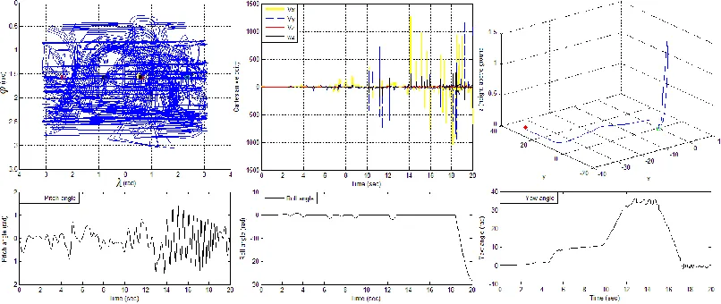
4.1 Case 1: Hovering Mission With The Nominal Controller Without The Effects Of Multiple Uncertainties
In this case, the multirotor MAV has to hover five meters above four target points without the effects of uncertainties by using the combination of the spherical IBVS and the nominal flight controller (velocity and attitude) without the robust compensator in the attitude loop. The multirotor MAV has initial position 𝜉 =
(0 0 0)𝑇. Figure 4 shows the corresponding responses.
As can be seen, the feature points have smooth trajectory path in the 𝜆𝜑 -space toward their desired position. Overall, the controller achieves good dynamical tracking performances for the nominal conditions.
4.2 Case 2: Hovering Mission With The Nominal Controller Under The Effects Of Multiple Uncertainties
The uncertainties are assumed as Gaussian noises with 250 mean and 1 variance values for 𝑞𝜃 only. 𝑞𝜙 and 𝑞𝜓 are assumed to be 0. The same controller as Case 1 is considered. As can be seen in Figure 5, if the uncertainties are considered, the response of the nominal controller can no longer track the reference signal and its tracking errors become larger without boundaries. As a result, the multirotor MAV was not able to hover above four target points.
Figure 4 Case 1: a) The path of the point features in the 𝜆𝜑 –space. “o” denotes initial position, “*” denotes the final position of
features. b) Spatial velocity components. c) Vehicle/ camera position in Cartesian space. “o” denotes initial position, “*” denotes the final position of features. d) Attitude response for pitch, roll, and yaw angles. Note: The arrangement of figures is [a b c; d].
Figure 5 Case 2: a) The path of the point features in the 𝜆𝜑 –space. “o” denotes initial position, “*” denotes the final position of
Figure 6 Case 3: a) The path of the point features in the 𝜆𝜑 –space. “o” denotes initial position, “*” denotes the final position of features. b) Spatial velocity components. c) Vehicle/ camera position in Cartesian space. “o” denotes initial position, “*” denotes the final position of features. d) Attitude response for pitch, roll, and yaw angles. Note: Arrangement of figures is [a b c; d]
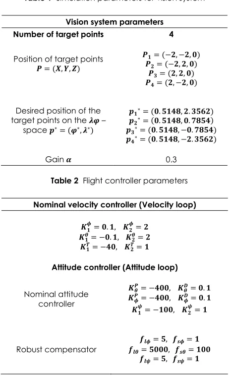
Table 1 Simulation parameters for vision system
Vision system parameters
Number of target points 4
Position of target points
𝑷 = (𝑿, 𝒀, 𝒁)
𝑷𝟏= (−𝟐, −𝟐, 𝟎)
𝑷𝟐= (−𝟐, 𝟐, 𝟎)
𝑷𝟑= (𝟐, 𝟐, 𝟎)
𝑷𝟒= (𝟐, −𝟐, 𝟎)
Desired position of the target points on the 𝝀𝝋 –
space 𝒑∗= (𝝋∗, 𝝀∗)
𝒑𝟏∗= (𝟎. 𝟓𝟏𝟒𝟖, 𝟐. 𝟑𝟓𝟔𝟐)
𝒑𝟐∗= (𝟎. 𝟓𝟏𝟒𝟖, 𝟎. 𝟕𝟖𝟓𝟒)
𝒑𝟑∗= (𝟎. 𝟓𝟏𝟒𝟖, −𝟎. 𝟕𝟖𝟓𝟒)
𝒑𝟒∗= (𝟎. 𝟓𝟏𝟒𝟖, −𝟐. 𝟑𝟓𝟔𝟐)
Gain 𝜶 0.3
Table 2 Flight controller parameters
Nominal velocity controller (Velocity loop)
𝑲𝟏𝝓= 𝟎. 𝟏, 𝑲 𝟐
𝝓= 𝟐
𝑲𝟏𝜽= −𝟎. 𝟏, 𝑲𝟐𝜽= 𝟐
𝑲𝟏𝑻= −𝟒𝟎, 𝑲𝟐𝑻= 𝟏 Attitude controller (Attitude loop)
Nominal attitude controller
𝑲𝜽𝑷= −𝟒𝟎𝟎, 𝑲𝜽𝑫= 𝟎. 𝟏
𝑲𝝓𝑷= −𝟒𝟎𝟎, 𝑲𝝓𝑫= 𝟎. 𝟏
𝑲𝟏𝝍= −𝟏𝟎𝟎, 𝑲𝟐𝝍= 𝟏
Robust compensator
𝒇𝒍𝝓= 𝟓, 𝒇𝒔𝝓= 𝟏
𝒇𝒍𝜽= 𝟓𝟎𝟎𝟎, 𝒇𝒔𝜽= 𝟏𝟎𝟎
𝒇𝒍𝝍= 𝟓, 𝒇𝒔𝝍= 𝟏
4.3 Case 3: Hovering Mission With The Proposed Controller Under The Effects Of Multiple Uncertainties
In this case, the robust compensator is integrated into the existing attitude closed-loop system with
parameters as presented in Table 2. As can be seen in Figure 6, the dynamical tracking performance of the closed-loop control system is extremely improved. The feature points have smooth trajectories in the 𝜆𝜑 – space toward their desired position and the multirotor MAV successfully hovered above the target points in Cartesian space and almost held to its horizontal position. The robust compensating signal for pitch subsystem 𝑢𝜽𝑅𝐶 successfully compensated the 𝑞𝜃 by sufficiently large parameters 𝑓𝑙𝜃 and 𝑓𝑠𝜃. If uncertainties are considered for roll and yaw subsystems, the behaviour is also similar with sufficiently large 𝑓𝑙𝑖 and 𝑓𝑠𝑖
(𝑖 = 𝜙, 𝜓).
5.0 CONCLUSION
This paper proposes an image-based robust hovering control of the multirotor MAV which considers the effects of multiple uncertainties in angular dynamics of vehicle. The proposed method is robust against uncertainties which contain external disturbances, nonlinear dynamics, coupling, and parametric uncertainties and does not require keeping target features in the field of view. The simulation results proved the effectiveness and robustness of the proposed closed-loop system.
This research aims for real-time implementation which is a challenging task due to uncertainties in image dynamics.
Acknowledgement
References
[1] Hutchinson, S., Hager, G. and Cork, P. 1996. A Tutorial on Visual Servo Control. IEEE Trans. Robotics and Automation. (63): 651-670.
[2] Hamel, T. and Mahony, R. 2002. Visual Servoing of an Underactuated Dynamic Rigid-Body System an Image Based Approach. IEEE Trans. Robotics and Automation. (18): 187-198.
[3] Mejias, L., Saripalli, S., Campoy, P., and Sukhatme, G. 2006. Visual servoing of An Autonomous Helicopter in Urban Areas Using Feature Tracking. Journal of Field Robotics. 23(3-4): 185-199.
[4] Saripalli, S., Sukhatme, G. S., Mejias, L. O., Cervera, P. C. 2005. Detection and Tracking of External Features in an Urban Environment Using an Autonomous Helicopter. IEEE International Conference on Robotics and Automation. 3972-3977.
[5] Peliti, P., Rosa, L., Oriolo, G., and Vendittelli, M. 2012. Vision-based Loitering over a Target for a fixed-Wing UAV. 10th International IFAC Symposium on Robot Control. (): 51-57. [6] Saunders, J. and Beard, R. 2008. Tracking a Target in Wind
Using a Micro Air Vehicle with a fixed Angle Camera. American Control Conference. 3863-3868.
[7] Bourquardez, O. and Chaumette, F. 2007. Visual Servoing of an Airplane for Alignment with Respect to a Runway. IEEE International Conference on Robotics and Automation. 1330-1335.
[8] Coutard, L., Chaumette, F., and Pflimlin, J. –M. 2011. Automatic landing on aircraft carrier by visual servoing. IEEE/RSJ International Conference on Intelligent Robots and Systems. 2843-2848.
[9] Bourquardez O. and Chaumette, F. 2007. Visual Servoing of an Airplane for autolanding. IEEE/RSJ International Conference on Intelligent Robots and Systems. 1314-1319. [10] Huh, S. and Shim, D. H. 2010. A Vision-based Automatic
Landing Method for fixed-wing UAVs. Journal of Intelligent and Robotic Systems. 217-231.
[11] Serra, P., Bras, F. L., Hamel, T., Silvestre, C., and Cunha, R. 2010. Nonlinear IBVS Controller for the flare Maneuver of fixed-wing Aircraft Using Optical flow. 49th IEEE Conference on Decision and Control. 1656-1661.
[12] Zhong, Y. 2002. Robust Output Tracking Control of SISO Plants with Multiple Operating Points and with Parametric and Unstructured Uncertainties. Int. J. Control. 75: 219–241. [13] Corke, P. . 2010. Spherical Image-based Visual Servo and
Structure Estimation. IEEE Int. Conf. on Robotics and Automation. 5550-5555.
[14] Castillo, P., Dzul, A., and Lozano, R. 2004. Real-time Stabilization and Tracking of a Four-rotor Mini Rotorcraft. IEEE Transactions on Control Systems Technology. 12(4): 510–516. [15] Pounds, P. 2007. Design, Construction, and Control of a Large
Quadrotor Micro Air Vehicle. PhD thesis, Australian National University.