ABSTRACT
DEY, SUMON. Design of a Scalable, Configurable, and Cluster-based Hierarchical Hardware Accelerator for a Cortically Inspired Algorithm and Recurrent Neural Networks. (Under the direction of Paul D. Franzon.)
Machine learning algorithms based on deep learning have met with enormous success to achieve higher performance in applications ranging from object recognition to defeating a hu-man expert in the complex game. Furthermore, it can broaden the horizon by processing a massive amount of multimodal natural data (video, audio) and learning useful join representa-tions in applicarepresenta-tions. In addition to deep learning, cortical learning algorithms can also learn representations in much closer to in a way a human brain works. Unlike the use of dense data in deep learning, binary data is used in cortical learning to model sparse distributed memory for different representations. These algorithms use artificial neural networks to model them into hardware. However, implementation of such networks in hardware relies on throughput and memory bandwidth of hardware architecture, which requires dealing with massive amount of data. To advance the research of these rapidly evolving techniques, there is a direct need for the design and implementation of specialized hardware to accelerate these algorithms.
© Copyright 2019 by Sumon Dey
Design of a Scalable, Configurable, and Cluster-based Hierarchical Hardware Accelerator for a Cortically Inspired Algorithm and Recurrent Neural Networks
by Sumon Dey
A dissertation submitted to the Graduate Faculty of North Carolina State University
in partial fulfillment of the requirements for the Degree of
Doctor of Philosophy
Computer Engineering
Raleigh, North Carolina
2019
APPROVED BY:
Winser Alexander Dror Baron
Eric Laber Paul D. Franzon
DEDICATION
BIOGRAPHY
Sumon Dey was born in September 1980, Mymensingh, Bangladesh. He received the bachelor’s degree in Electrical and Electronic Engineering from Bangladesh University of Engineering and Technology (BUET), Dhaka, Bangladesh, in 2004, and the master’s degree in Electrical and Computer Engineering from University of Illinois at Chicago (UIC), USA, in 2012. After graduating from BUET, he worked as a Network Switching Subsystem Engineer from 2004 to 2010 on GSM Network Architecture, OSI Reference Model, Interconnection, and Signaling Protocols at Telecommunication Industry, Dhaka, Bangladesh. During his masters, he worked as a research assistant at the Nanoengineering Research Laboratory (NRL), Chicago, USA. He began work towards his Ph.D. in Computer Engineering in Spring 2013.
ACKNOWLEDGEMENTS
Joining the Ph.D. program in the Department of Electrical and Computer Engineering at North Carolina State University was one of the best decisions of my life. I am especially indebted to my advisor, Paul D. Franzon, who has provided the opportunity to work with him. I am also thankful to him for introducing me to research centered on building hardware for next-generation artificial intelligence. He is an excellent advisor who gave me continuous support of my Ph.D. studies and research, gave me the freedom and encouragement to pursue my ideas and goals. More importantly, his patience, enthusiasm, and knowledge helped me throughout my graduate studies. I am thankful to Winser Alexander for his guidance and encouragement during my teaching assistantship of his course. I would like to thank Winser Alexander, Dror Baron, and Eric Laber for serving on my committee and agreeing to read my dissertation so quickly.
I was also fortunate to be a part of Cognitive Computing research group at Microelectronics Systems Laboratory (MSL) and would like to thank my colleagues, Steve Lipa, Lee Baker, Josh Schabel, Weifu Li, Josh Stevens, and Zachary Johnston for stimulating discussions, debates and continuous support for my research. A very special thanks goes to Steve Lipa for all of his help and support on design kits. My sincere thanks also go to Josh Schabel for giving me support on design kits, scripts, and helping me debug issues of different design flows. I thank Lee Baker for brainstorming discussions, exciting research debates, and also for benchmarking Sparsey on parallel computing platform through software implementation. I thank Weifu Li for discussing various properties and implementation aspects of the Hierarchical Temporal Memory algorithm. I would also like to thank Gerard (Rod) Rinkus, President of Neurithmic Systems, for his interesting discussions and continuous updates on Sparsey.
TABLE OF CONTENTS
LIST OF TABLES . . . vii
LIST OF FIGURES . . . ix
Chapter 1 Introduction . . . 1
1.1 Motivation . . . 3
1.2 Contribution and Outline . . . 5
1.3 Abbreviations . . . 7
Chapter 2 Background. . . 9
2.1 Fundamental of Artificial Neural Networks . . . 9
2.2 Target Neural Networks . . . 13
2.2.1 Sparsey . . . 13
2.2.2 Long Short-Term Memory . . . 17
2.3 Development of Neural Networks . . . 22
Chapter 3 State-of-the-art . . . 23
3.1 Introduction . . . 23
3.2 Hardware Plaforms . . . 23
3.2.1 General Purpose Processor . . . 23
3.2.2 Field-Programmable Gate Array . . . 24
3.2.3 Custom Hardware . . . 24
3.2.4 Domain-specific Processor . . . 25
3.3 Conclusion . . . 26
Chapter 4 A Custom Hardware for Sparsey . . . 27
4.1 Introduction . . . 27
4.2 Design Space Exploration . . . 27
4.2.1 Computation . . . 28
4.2.2 Memory . . . 28
4.2.3 Precision . . . 30
4.2.4 Configurability . . . 31
4.2.5 Communication . . . 31
4.3 Hardware Implementation Details . . . 32
4.3.1 Cluster . . . 32
4.3.2 Processing Element . . . 33
4.3.3 Network-on-chip . . . 37
4.4 Experimental Setup . . . 39
4.5 Results . . . 41
4.6 Discussion . . . 44
4.6.1 Inter-cluster Communication . . . 44
4.6.2 Scalability . . . 44
Chapter 5 An ASIP for RNNs. . . 47
5.1 Introduction . . . 47
5.2 Design Space Exploration . . . 48
5.2.1 Computation . . . 48
5.2.2 Memory . . . 48
5.2.3 Mapping Networks onto Hardware . . . 51
5.2.4 Precision . . . 54
5.3 Hardware Implementation Details . . . 56
5.3.1 System Overview . . . 56
5.3.2 Memory and Data Allocation . . . 58
5.3.3 Processing Element . . . 63
5.3.4 Instructions . . . 79
5.3.5 Data Reuse . . . 80
5.3.6 Compiler . . . 80
5.4 Experimental Setup . . . 81
5.5 Results . . . 83
5.6 Discussion . . . 89
5.6.1 Flexibility . . . 89
5.6.2 Scalability . . . 89
5.7 Conclusion . . . 90
Chapter 6 Conclusion and Future Work . . . 91
6.1 Summary of Contributions . . . 92
6.2 Future Work . . . 93
References. . . 95
Appendices . . . .105
Appendix A Sparsey . . . 106
A.1 Mathematical Steps of CSA . . . 106
A.2 Comparision with DNN . . . 110
Appendix B LSU of ASIP . . . 111
B.1 Instruction of Load and Store . . . 111
Appendix C SFU of ASIP . . . 114
C.1 Pseudocode of Special Function . . . 114
LIST OF TABLES
Table 4.1 The range and format of different parameters for this accelerator . . . 30
Table 4.2 The configurable units of a PE . . . 31
Table 4.3 The configuration of 2-D mesh NoC in this design . . . 38
Table 4.4 The configuration of global NoC in scalability studies . . . 38
Table 4.5 The baseline network of three-layer Sparsey . . . 39
Table 4.6 The hardware specification of Tesla P100 GPU . . . 40
Table 4.7 The total on-chip SRAM requirement for a cluster . . . 40
Table 4.8 The key hardware results of a PE . . . 41
Table 4.9 The hardware results of a cluster . . . 42
Table 4.10 The area, power, and bandwidth comparision against GPU . . . 42
Table 4.11 The processing time of GPU and this work . . . 43
Table 4.12 The operations per second comparision for hotspot processing . . . 43
Table 5.1 The access latency per operation . . . 59
Table 5.2 The energy comsumption per operation . . . 59
Table 5.3 The instruction format of DMA lane . . . 67
Table 5.4 The address of DMA lane . . . 67
Table 5.5 The available opcodes of DMA instruction . . . 67
Table 5.6 The source and destination address . . . 68
Table 5.7 The register mapping of DMA instruction . . . 68
Table 5.8 The instruction format of LSU lane . . . 71
Table 5.9 The address of LSU lane . . . 71
Table 5.10 The available opcodes of LSU instruction . . . 71
Table 5.11 The instruction format of VFU lane . . . 72
Table 5.12 The address of VFU lane . . . 72
Table 5.13 The available opcodes of VFU instruction . . . 73
Table 5.14 The instruction format of SAU lane . . . 75
Table 5.15 The address of SAU lane . . . 75
Table 5.16 The available opcodes of SAU instruction . . . 75
Table 5.17 The instruction format of SFU lane . . . 77
Table 5.18 The address of SFU lane . . . 77
Table 5.19 The available opcodes of SFU instruction . . . 77
Table 5.20 The status of functional unit . . . 78
Table 5.21 The status of SRAM bank . . . 78
Table 5.22 The status of register files . . . 79
Table 5.23 The example of high level functions and corresponding instructions . . . 81
Table 5.24 The hardware specification of Tesla P100 GPU . . . 82
Table 5.25 The key hardware results of a PE . . . 83
Table 5.26 The area comparison . . . 84
Table 5.27 The speed and power comparison for batch processing . . . 84
Table 5.28 The speed and power comparison for online processing . . . 85
Table 5.30 The operations per second comparison for batch processing . . . 86
Table 5.31 The operations per second comparison for online processing . . . 86
Table 5.32 The number of instructions for batch processing . . . 87
Table 5.33 The number of instructions for online processing . . . 88
Table 5.34 The number of instructions for Adam optimizer . . . 88
Table A.1 The fundamental differences between Sparsey and DNN . . . 110
Table B.1 The no operation instruction . . . 111
Table B.2 The load instruction from SRAM to vreg . . . 112
Table B.3 The store instruction from vreg to SRAM . . . 112
Table B.4 The load instruction from SRAM to hreg . . . 112
Table B.5 The store instruction from hreg to SRAM . . . 112
Table B.6 The load instruction from SRAM to vreg . . . 112
Table B.7 The load instruction from SRAM to hreg . . . 112
Table B.8 The load instruction from sreg to SRAM . . . 113
Table C.1 The constants of polynomial . . . 116
LIST OF FIGURES
Figure 2.1 A biological neuron . . . 10
Figure 2.2 A perceptron or artificial neuron . . . 11
Figure 2.3 A multilayer perceptron (MLP) neural network . . . 12
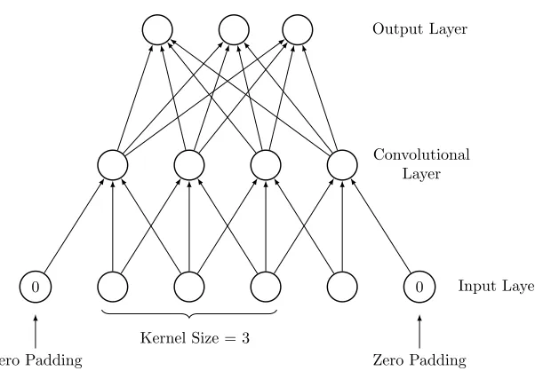
Figure 2.4 A 1D convolutional neural network (CNN) for stride of one . . . 12
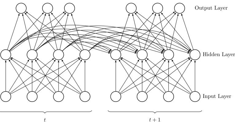
Figure 2.5 A recurrent neural network (RNN) . . . 13
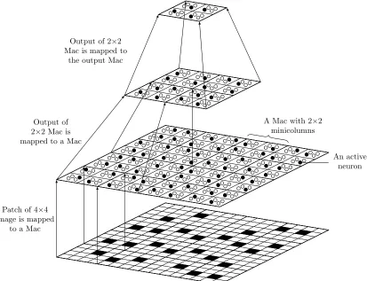
Figure 2.6 A three-layer Sparsey network . . . 14
Figure 2.7 A single layer LSTM network . . . 18
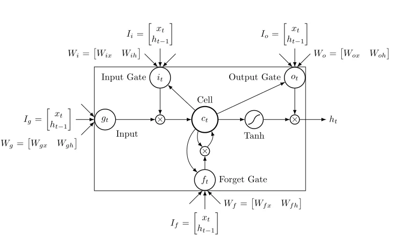
Figure 2.8 An LSTM Unit . . . 18
Figure 4.1 The hardware architecture of a cluster . . . 33
Figure 4.2 The hardware architecture of a PE . . . 34
Figure 4.3 The hardware architecture of a CM . . . 35
Figure 4.4 The hardware architecture of a neuron . . . 36
Figure 4.5 The hardware architecture of multiply-accumulate submodule . . . 37
Figure 4.6 The global interconnection network connects 16 clusters . . . 45
Figure 4.7 The performance and scalability of hierarchical accelerator . . . 45
Figure 5.1 Matrix multiplication using block matrix . . . 50
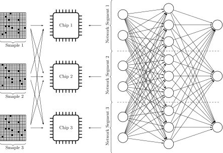
Figure 5.2 Model parallelism of network in hardware . . . 52
Figure 5.3 Data parallelism of network in hardware . . . 53
Figure 5.4 The top-level concept of mixed precision training . . . 55
Figure 5.5 The overall architecture of proposed system . . . 56
Figure 5.6 PEs connected to DiRAM4 banks using crossbar . . . 57
Figure 5.7 A single bank of DiRAM4 3D memory . . . 59
Figure 5.8 The configuration of DiRAM4 bank for version burst of 2 . . . 61
Figure 5.9 The sorage and access pattern of a DiRAM4 bank . . . 62
Figure 5.10 The overall architecture of a PE . . . 64
Figure 5.11 The architecture of programmable DMA controller . . . 66
Figure 5.12 The dataflow of DMA operations . . . 69
Figure 5.13 The architecture of Vector Functional Unit (VFU) . . . 73
Figure 5.14 The architecture of Scalar Arithmetic Unit (SAU) . . . 74
Chapter 1
Introduction
Machine learning algorithms have enjoyed enormous success in many modern applications rang-ing from healthcare to e-commerce to social network, etc [1, 2, 3, 4]. The most common form of machine learning is deep learning, which can process natural data. In recent years, deep learning algorithms have outperformed most other machine learning algorithms especially in pattern-recognition, natural language processing, navigation (self-driving cars), and cybersecu-rity [5, 6, 7, 8, 9]. Deep learning using deep neural networks (DNNs) have achieved revolutionary success in learning and recognition of spatial context and temporal sequences, respectively, from raw natural data [5]. Over the last few years, the accuracy of these applications has rapidly improved by using larger network sizes. The classification accuracy of visual object recognition (top-1 accuracy) has increased 62.5% in 2012 to 80.0% in 2016 using AlexNet and Inception-v4, respectively, on ImageNet dataset [10, 11]. On the other hand, the automated transla-tion (English-to-French, English-to-German) system used the deep Long Short-Term Memory (LSTM) and reduced the translation error by 60% compared to the Google’s phrase-based sys-tem [12, 13, 14]. However, these algorithms work only on labeled data provided that the training set is labeled with the expected prediction. For example, each photo of a cat presented to a DNN is clearly labeled “cat”, which referred to as supervised learning. Cortical learning algorithm (CLA), that can learn with minimal or no supervision on lightly labeled data or completely unlabeled data, are gaining interest. These algorithms process data in a manner much closer to the way a human brain learns. The recent implementation of these algorithms shows promising success and getting much attention for its ability to understand the spatio-temporal pattern [15, 16].
Inception-v4) increased the computation 16.14 times (2 billion to 22.6 billion operations) with slightly decreased the parameter sizes (approximately 2.5 times) where the size of a single image is 224×224 (real-life image size 1600×1200) [10, 11]. The increased model size also increases the inference time per image 18ms to 150ms (approximately eight times) on NVIDIA K40 GPU [17]. The inference accuracy improvement of machine translation (English to France) using LSTM also comes at the price of a network with huge parameters (384 million) and computation is approximately 4 TOPS to process words [14, 18]. However, the number of computations is highly dependent on the mini-batch size and the hidden size. In addition to computation, the network parameters have also increased 88 times (4.3 million to 384 million) from 2013 to 2015 in language processing task [6, 18]. The training of image recognition and machine translation models also takes between six to ten days and involves multiple graphics processor units (GPUs) to enhance data storage and memory bandwidth [10, 14]. On the other hand, the tiny version of a cortical algorithm implements 7×10⁴ neurons with 1.54 million synapses, as compared to the human brain has approximately 2×10¹⁰neurons and approximately 5×10¹⁴ synapses. This small model also requires approximately 3.08 million operations to process a single 16×24 image [19].
In addition to computation and memory resources, power consummation is another key challenge that limits the implementation of these networks in hardware. In CLA, parameters of the network are binary, sparse and require less storage compared to the dense and floating-point parameters. However, the number of neurons is much higher than that of RNNs [20]. Thus the use of on-chip memory for synaptic weights can reduce the access energy, in other words, meet the power budget of the hardware. In contrast to CLA, RNNs use to model deep learning algorithms have a smaller number of neurons with large dense floating-point parame-ters, which requires the use of the off-chip memory of GPUs to store parameters (samples and weights) and access huge amount of data for training and inference. Running these networks on multiple GPUs (up to 8) requires almost 235W to 2000W in power consumption [10, 14]. Also, GPUs are designed for general purpose computation and not optimized for the performance of these algorithms. The overall power overhead of these networks on general purpose hardware is significant. Therefore, specialized hardware can benefit enormously by improving the power budget of these algorithms.
networks (RNNs) using the emerging high bandwidth and low energy off-chip 3D memory. The ASIP solution is designed in a way to support both training and inference of RNNs and poten-tially others. The hardware is used to process the popular Google’s Neural Machine Translation System. It performed training and inference for different batch configuration and achieved an overall 6.5×– 61.0×performance improvement than a Tesla P100 GPU [22].
1.1
Motivation
One algorithm that can learn in unsupervised or lightly supervised mode is the Neurithmic’s Sparsey algorithm [23]. Sparsey is a scalable online probabilistic cortical algorithm inspired by the cortical column of a brain and seeks to mimic the essential computational properties of the neocortex. The initial implementation of Sparsey achieved 91% recognition accuracy on MNIST dataset [19, 24, 25]. The primary goal of Sparsey is to model human episodic memory, that is, the memory of specific events. It memorizes patterns in a sparse distributed representation (SDR) network by increasing the connections – the weights in an SDR are binary. In Sparsey, any input pattern activates only a small fraction of the total neurons. It is anticipated that Sparsey would not perform well on GPUs because GPUs are optimized for computations of dense matrices on floating-point data and Sparsey requires massive multiply-accumulate (MAC) operations on sparse binary data.
Sparsey uses a neural network where the total number of neurons is large and while only a fraction of total neurons are active, every neuron needs to access its own binary weight matrices in each neural cycle. This computation requires a large memory bandwidth to obtain synaptic weights simultaneously whereas GPU has limited on-chip storage with huge memory bandwidth but a substantial off-chip memory with limited memory bandwidth. The total size of weight matrix of a single neuron is relatively small (compared to a floating-point weight matrix) and can fit in the on-chip SRAM, which is faster to access (increases memory bandwidth) than the off-chip memory of GPUs. Sparsey also learns in an online manner, which demands high-speed processing for each incremental training cycle (approximately 16 ms/frame) in hardware.
To map sizeable Sparsey networks onto GPUs requires significant memory bandwidth to read (or write) the off-chip weight matrices and increase the energy consumption. The memory access rate is the bottleneck in Sparsey and dominates the overall power consummation and limits the performance needed to implement the sizable Sparsey network on a GPU. The access energy can be reduced approximately 130 times (640 pJ/word to 5 pJ/word in 45nm technology) using on-chip SRAM [26].
floating-point operations. However, each neural cycle also requires some floating-floating-point operations and special function operations. The fixed-point hardware implementations of these floating-point operations and special function operations can decrease the overall area and power (13.6× and 21.5×in 45nm, respectively) and helps to accommodate more neurons in silicon [26]. The primary motivation of this work is to estimate the meaningful upper bound performance of an ASIC compared to the peak hardware performance of state-of-the-art GPUs.
Performance and flexibility are the two significant requirements of hardware architecture needed to implement Convolutional neural network (CNN) and different variants of recurrent neural network (RNN). The architecture community has mainly focused on CNN, with little attention to RNNs or MLPs, where CNN only process tiny portion of the workload in the complete system [27]. Indeed, most of the hardware research on RNNs has focused on the inference engine where training is still heavily involved with multiple GPUs. One of the primary motivations of ASIP accelerator of RNNs is to fill that research gap and implement flexible hardware for training as well as inference.
The training of state-of-the-art RNNs runs on multiple GPUs and takes more than a week. A single forward propagation of training involved an estimated 2 TFOPS and 12 Tb/s memory bandwidth [14]. The parameters of RNNs are floating-point, dense matrices and cannot be stored in on-chip. Thus, the computations are mostly depended on the off-chip memory bandwidth. The appropriate level of floating-point hardware resources is also required to accelerate the training and inference for different hyperparameters.
State-of-the-art RNNs have millions of parameters (384 million) and requires massive amount of storage and computational resources for training and inference [13, 14]. To fetch 384 mil-lion parameters (approximately 12 Gb) from off-chip memory requires almost 14.6 W of power considering conditions at 60 fps and 640 pJ access energy [26]. The training dataset also needs to access from off-chip memory during training. The computation of training is usually done in single-precision floating-point to maintain training accuracy, which also increases the overall power consumption in GPUs or similar hardware platforms.
Flexibility of hardware is essential because RNN has different variants and the data flow of different deep learning networks can be different. In addition, an application specific RNN shows better performance accuracy compared to generic RNNs. Thus, a new hardware solution is required to improve training time, react in a faster manner to real-life inputs, and keep up with the change of algorithms and network variants. Flexibility of hardware is also required to map networks into hardware in a different fashion (model parallelism, data parallelism, etc.) and achieve higher performance [28, 29].
arith-metic is area and power efficient (14.45× and 7.6×, respectively) and significantly decreases the total area budget [26]. Unfortunately, half-precision training loses the training accuracy (convergence) for some variants of DNNs. However, the mixed precision training, combination of single-precision and half-precision, can maintain training accuracy as good as single-precision in hardware and also can reduce the area of silicon [30].
The data flow of RNNs is another important reason to design hardware. The training of RNNs has a pattern of irregular data access from the off-chip memory (i.e. DRAM) instead of contiguous behaviors. The irregular pattern of memory access makes DRAM much harder to operate on burst mode and maintain the highest DRAM bandwidth during training. Thus, mapping the network parameters to a DRAM and associated functionality in the hardware could increase the memory bandwidth and accelerate the training of RNNs.
These are the motivational factors which led to the design of custom hardware (ASIC) for Sparsey and an application-specific instruction set processor (ASIP) for RNNs targeting both training and inference.
1.2
Contribution and Outline
A benchmark of a three-layer Sparsey of 336×103neurons is implemented in a GPU-accelerated parallel computing platform that analyzes different aspects to optimize algorithm into custom hardware. The key contributions of this work are the following innovations specifically designed to create an efficient engine on which to execute Sparsey:
• A distributed on-chip memory technique that consists of storage associated with each neuron for synaptic weights and on-chip shared memory, which increases the bandwidth utilization 91.75× compared to a GPU.
• A special multiply-accumulate (MAC) technique that consists of binary dot product fol-lowed by mixed-width integer accumulations, dedicated to the on-chip memory of neurons, which efficiently utilize the bandwidth of on-chip memory and accelerate the hotspot op-eration of Sparsey.
• Fixed-point custom hardware for arithmetic, a special function unit (SFU), and network-on-chip (NoC) based on data flow of Sparsey that can further reduce the area and power of the custom hardware.
• An efficient custom hardware of Sparsey that can learn and recognize events of KTH action recognition dataset and achieve 25.24× speedup, 1.43× reduction in area, and 353.12× energy efficiency against a Tesla P100 GPU.
A novel application-specific instruction set processor (ASIP) is designed analyzing different aspects of the recurrent neural networks to improve performance on hardware. The contributions of this work are:
• An emerging 3D-stacked memory to increase the off-chip memory bandwidth and a sized on-chip memory to enhance data locality for reducing long latency off-chip memory access and accelerating the algorithm.
• A set of short instructions designed after analyzing data flow of different complex, time-consuming, special operations into high-level function blocks for training and inference of RNN variants to improve the flexibility of hardware.
• A state-of-the-art training technique, called mixed precision training that consists of half-precision multiplier followed by the single-half-precision adder, which can improve the hard-ware performance maintaining the training accuracy similar to the single-precision. • A look-up table (LUT) technique, a combination of on-chip memory based LUT and
fast numerical method and associated high-level instructions, that can compute different operations (divider, square root, log) and also non-linear activation (Sigmoid, Tanh, etc.) to improve the performance in hardware.
• A high-level programming environment to generate Very Long Instruction Word (VLIW) instructions for this ASIP architecture and process RNN variants.
• An efficient ASIP architecture that can perform both training and inference of RNNs and MLPs by increasing the memory bandwidth and parallelism at different levels. This work processed training and inference of language modeling task, and achieved 1.5× – 5.6×
processing speedup, 4.3× – 40.8× reduction in energy, and 1.5× area reduction than a Tesla P100 GPU.
The remaining chapters of this dissertation are organized as follows:
Chapter 2 provides the fundamentals of neural networks, the learning (or training) algo-rithms of Sparsey and Long Short-Term Memory (LSTM), one of the most popular and suc-cessful variants of RNN. The most recent real-world applications of LSTM and success stories of Sparsey are also discussed briefly in this chapter.
Chapter 4 presents the ASIC solution of Sparsey. This chapter starts with a discussion of the various algorithmic aspects of Sparsey in hardware needed to consider during designing of the custom hardware. The implementation details and experimental setup are presented in the subsequent sections. The speedup and energy efficiency of ASIC compared to a GPU are presented in the result section. The scalability studies are shown in the discussion section.
Chapter 5presents the ASIP solution of RNNs. The algorithmic aspects, mapping networks in hardware, memory access pattern of RNNs are analyzed before giving the details of hardware implementation. It also discusses the experimental setup to estimate performance improvement against a GPU. This chapter also discusses the flexibility and scalability of the proposed ASIP architecture.
Chapter 6 summarizes the dissertation by discussing the lessons learned, the future work of deep learning accelerators, and presents a conclusion.
1.3
Abbreviations
ML Machine Learning DL Deep Learning
CLA Cortical Learning Algorithm AN Artificial Neuron
ANN Artificial Neural Network
RNN Recurrent Neural Network MLP Multilayer Perceptron
CNN Convolutional Neural Network
DNN Deep Neural Network GRU Gated Recurrent Unit LSTM Long Short-Term Memory
VLIW Very Long Instruction Word SDR Sparse Distributed Representation SDM Sparse Distributed Memory
Mac Macrocolumn
CM Competitive Module
CSA Code Selection Algorithm
SISC Similar-Inputs-to-Similar-Codes
FC Fully Connected
GD Gradient Descent
SGD Stochastic Gradient Descent
BPTT Backpropagation Through Time
FV Feature vector
MAC Multiply-Accumulate
SRAM Static Random-Access Memory
DRAM Dynamic Random-Access Memory
ASIC Application-Specific Integrated Circuit
ASIP Application-Specific Instruction Set Processor
GPU Graphics Processing Unit
TPU Tensor Processing Unit
FPGA Field-Programmable Gate Array
PE Processing Element
NoC Network-on-Chip
SFU Special Function Unit
DSDR Dual Single Data Rate
Chapter 2
Background
The fundamental of neural networks, target neural networks, how they work, and some recent applications are discussed in this chapter. Both cortical learning and deep learning algorithms use an artificial neural network (ANN) to solve various machine learning tasks. An artificial neural network is a collection of neurons (or compute unit) that are connected in various fashions. The fundamental properties (number of neurons, storage, connection types, etc.) of ANN varies depending on whether it is used for cortical learning or deep learning applications. The cortical learning uses ANN to build a mathematical model (sparse distributed memory) of the neocortex and uses that model to learn (or recognize) events. This type of ANN usually uses binary connections, and a massive number of neurons. However, at one time, only a few fractions of neurons are active (or fired) to generate sparse binary code for Hebbian learning [20, 31]. It also uses multiple layers of neurons stacked vertically in what is called deep neural network (DNN); the number of multiple layers is limited by the layers of the neocortex (usually 6) [31]. On the contrary, DNNs inspired by deep learning use multiple layers (can be more than 6) of neurons, but there are fewer number of neurons per layer than that of CLA [10, 11]. In addition, DNN uses float connections between neurons and float vector to represent an event. These types of DNNs often works on labeled data and requires an optimizer (Gradient Descent) to learn the strength of connections [32].
2.1
Fundamental of Artificial Neural Networks
Nucleus
Cell body Axon
Axon terminals Dendrites
Figure 2.1: A biological neuron
Neurons communicate with each other through synapses that usually formed between axon terminals (multiple terminals of an axon) of one neuron and dendrite of another neuron. The cell body of a neuron performs the summation of incoming signals from synapses and fires (send an impulse to other neurons through axon) only if the summation reaches its threshold value.
A mathematical model of a biological neuron, artificial neuron (AN), is shown in Figure 2.2. An artificial neuron (AN) is the basic building block or compute unit of an ANN. It con-sists of three primary components that include synaptic weights, a threshold, and an activation function. The synaptic weights (W) are factors associated with each input and determine the strength of the input vector (X) by multiplying the weight matrix and input vector (WTX). There is an internal threshold in AN, called bias, added to the weighted-input (WTX) and can affect the activation of the output. The weighted-input is then passed through an activation function to produce the output and transmitted to other neurons similar to the way the biolog-ical neuron propagates the summation of the incoming signal to other neurons through axon. There are different types of activation functions (Sigmoid, Tanh, ReLU, etc.) used in ANNs and the primary purpose of using activation function is to introduce non-linear properties in ANN. In ANN, there is one input layer, one output layer, and one (or multiple) hidden layer(s). DNNs are simply neural networks with more than one hidden layer. For simplicity, the rest of the dissertation will refer to artificial neuron (AN) as neuron and artificial neural network (ANN) as neural network.
Activation function
P
Summation
w2
x2
.. . .. . .. .
wn xn
w1
x1
w0
x0
inputs weights
Figure 2.2: A perceptron or artificial neuron
Tensor Processing Unit (TPU), deployed in the datacenter, represents 61% of its workload for MLP [27]. In addition to MLP, there is another type of feedforward neural network, Convo-lutional Neural Network (CNN, or ConvNet), are mostly applied to analyzing visual imagery. Unlike MLP, a CNN has spatial locality of input signals and shared weights in space which makes the number of weight parameters much smaller than a fully-connected layer. Due to data locality and reusability in CNN, it is usually computation bound rather than data bound. Hardware implementation of CNN in TPU shows only 5% of Google’s datacenter workload [27]. A special non-linear activation function, which is computationally less expensive in hardware called Rectifier Liner Unit (ReLU) is often used to accelerate MLP and CNN in hardware [27, 33]. Both MLP and CNN map input to output (or activations), which is known as feature mapping or activation mapping. A different type of neural network, Recurrent Neural Network (RNN), can map the history of previous inputs to output activations and can be applied to solve sequential prediction problems (Speech, Video). Two types of connections (feed-forward and feedback) are usually present among neurons in RNN. However, there are many variants of RNN based on their connectivity. In RNN, there are internal states or memories that used to process or summarize the history. The feedback connections that are ubiquitous in the human brain are inspired researcher to model neocortex using different variants of RNN and performs sequence processing tasks similar to the human brain. From the hardware perspective, opera-tions per weight are lower in RNN, which makes it memory bound rather than computation bound. Thus, the implementation of RNN in hardware is less efficient because hardware is rela-tively cheap for computation than fetching data. Long Short-Term Memory (LSTM), a popular variant of RNNs, implemented on TPU processes 29% of Google’s datacenter workload [27].
Input Layer Hidden Layer Output Layer
Figure 2.3: A multilayer perceptron (MLP) neural network
0 0
Zero Padding Zero Padding
Kernel Size = 3
Input Layer Convolutional
Layer Output Layer
t t+ 1
Input Layer Hidden Layer Output Layer
Figure 2.5: A recurrent neural network (RNN)
an unsupervised manner based on “unlabeled” data. For instance, Auto-encoders and Genera-tive Adversarial Networks (GANs) are two useful variants of CNN that perform unsupervised training [34, 35]. Unsupervised learning is also used to train LSTM for discriminating different types of sequences [36]. In addition, brain-inspired recurrent networks (Hierarchical Temporal Memory (HTM), Sparsey, Cogent Confabulation) also use unsupervised learning on binary in-put data [20, 37, 38]. The basic connectivity of MLP, CNN and RNN are shown in Figure 2.3, Figure 2.4, and Figure 2.5, respectively. In these figures, RNN clearly shows a much higher number of connections than others.
2.2
Target Neural Networks
The target neural network architectures of hardware implementation are discussed in this sec-tion. A brain-inspired neural network (Sparsey) can learn unsupervised, and a successful variant of RNN, LSTM, can learn in supervised fashion are chosen for hardware acceleration.
2.2.1 Sparsey
Basic Concepts of the Sparsey Network
The neuron is the basic computational unit of the Sparsey network just like other neural net-works. A single neuron has three types of connections (bottom-up (U), horizontal (H), and top-down (D)) where connections (or synapses) have binary weights. The signal propagating in the bottom-up and top-down connections carry the spatial information and the horizontal connections carry the temporal information. The weights of connections are updated using the Hebbian learning rule [37]. There is also an activation function (usually Sigmoid) associated with each neuron. In Sparsey, neurons are arranged in minicolumns, minicolumns organized in macrocolumns, and macrocolumns in layers. The minicolumn is considered analogous to a spe-cific portion – the pool of layer∼20 2/3 pyramidal neurons – of the human cortical minicolumn [37]. Minicolumns and macrocolumns are also referred to as competitive modules (CM) and mac (Mac), respectively. A three-layer Sparsey network is shown in Figure 2.6.
Patch of 4×4 image is mapped
to a Mac Output of 2×2 Mac is mapped to a Mac
Output of 2×2 Mac is mapped to
the output Mac
A Mac with 2×2 minicolumns
An active neuron
Properties of Sparsey Network
The interesting properties of Sparsey are: 1) it has similar-inputs-to-similar-codes (SISC) prop-erty i.e. it learns in an unsupervised manner and uses CSA to select highly intersecting sparse distributed codes (SDCs) for matching to similar inputs; 2) it forms long-lasting memory traces of sequences based on single unsupervised learning of each sequence; 3) the number of computa-tional steps needed to either learn a new frame or retrieve (recognize) a previously learned frame remains constant for the life of system regardless of the information stored in the system; 4) it can recognize an individual training sequence (exactly or slightly perturbed version) prompted with the first frame of the sequence; and 5) it can recognize the novel sequences compared to the closely approximated versions of known sequences.
Algorithms of Sparsey
The core algorithm of Sparsey has two different modes of operations: 1) learning or training mode; and 2) inference or recognition mode. The CSA choose one neuron from each CM to generate an SDC corresponding to Sparsey’s input feature vectors during both learning and inference mode.
In learning mode, a Mac becomes active if either the number of active features (or active bits) of bottom-up connections lies within specified limits or it is already active for the number of frames that is less than its persistence. The persistence is the activation duration of Mac in each layer, which is usually increased in upper layers of the model. Every neuron (K) of a layer performs the summation of weighted inputs independently for different types of connections (bottom-up, horizontal, and top-down) followed by normalization each summation. Neurons then compute in a three-way match (the overall local measure of support (V)) for different input sources followed by calculating the highest local support in each CM (Q). The highest local support is used to calculate various parameters (η,G, etc.) of the non-linear activation function. The non-linear activation function, Sigmoid, is used to calculate the relative probability of winning (ψ) for each neuron before the softmax operation. A winner neuron is selected from each CM using a random number determined by applying the probability distributions (ρ) of neurons’ winning in that CM. The learning rule is applied updating the weights leading to and from the winning neurons [37]. In Sparsey, the freezing of learning, based on a threshold, is applied to each Mac to limit the saturation. The detail aspects of the freezing mechanism at different levels are still under exploration [37].
Algorithm 2.1:The Code Section Algorithm (CSA) during Learning for episode←0 to T do
if M = active then forj←0 to Qdo
fori←0 to K do
u(i)←(Px(t−0).w,∀(x, w)∈(Xu, Wu))
h(i)←(Px(t−1).w,∀(x, w)∈(Xh, Wh))
d(i)←(Px(t−1).w,∀(x, w)∈(Xd, Wd))
U(i), H(i), D(i)←Normalize(u(i), h(i), d(i)) if t6= 0 then
Local Support(V(i))←U(i).H(i).D(i) else
Local Support(V(i))←U(i) end if
end for end for
forj←0 to Qdo
V(j)←Max(V(i)),∀i∈j
end for
Parameters of Sigmoid(G, η)←(V(j), Q, K) forj←0 to Qdo
fori←0 to K do
ψ(i)←Sigmoid(V(i), G, η) end for
end for
forj←0 to Qdo fori←0 to K do
ρ(i)←Softmax(ψ(i)) end for
end for
forj←0 to Qdo
Select a Winner←Winner-take-all(ρ(i)) Update Weights←Hebbian Learning end for
Algorithm 2.2:The Code Section Algorithm (CSA) during Inference for episode←0 to T do
if M = active then forj←0 to Qdo
fori←0 to K do
u(i)←(Px(t−0).w,∀(x, w)∈(Xu, Wu))
h(i)←(Px(t−1).w,∀(x, w)∈(Xh, Wh))
d(i)←(Px(t−1).w,∀(x, w)∈(Xd, Wd))
U(i), H(i), D(i)←Normalize(u(i), h(i), d(i)) if t6= 0 then
Local Support(V(i))←U(i).H(i).D(i) else
Local Support(V(i))←U(i) end if
end for end for
Maximum Likelihood Estimation←V(i) else
return end if end for
with the back-off policy currently under exploration [37]. The deterministic algorithm called the “maximum likelihood” method is much faster since it obviates the later steps of the CSA and for many applications, it yields much better performance and higher expected accuracy [37]. Algorithm 2.1 and Algorithm 2.2 explains the learning and inference steps of the CSA, respectively.
2.2.2 Long Short-Term Memory
t t+ 1
Input Layer LSTM Layer Output Layer
LSTM Unit
Figure 2.7: A single layer LSTM network
ct Cell
Tanh
× ht
× gt
×
ft Forget Gate it
Input Gate Output Gate ot
Input
Ig =
xt ht−1
Wg=Wgx Wgh
Ii=
xt ht−1
Wi=Wix Wih
Io=
xt ht−1
Wo =Wox Woh
If =
xt ht−1
Wf =
Wf x Wf h
Basic Concepts of LSTM Network
Memory cell or LSTM unit (shortly unit) is the basic computational unit arranged in layers. A single unit is guarded by three different multiplicative gates known as input gate, output gate, and forget gate. The multiplicative input gate usually protects the unit (or memory content) from irrelevant inputs, and the multiplicative output gate protects other units from the currently perturbed unit. The multiplicative forget gate protects the unit from the irrelevant past content (memory state) by resetting it at an appropriate time [40]. A single unit and associated gates usually have connections (or weight parameters) from an input and also from itself. In addition to units arranged in stacked LSTM layers, there are also output units arranged in the one or multiple output layers. An output unit usually has connections from all outputs (or activations) of the subjacent layer [i.e. output layer is usually fully-connected (FC)]. Similar to the perceptron, a non-linear activation function (Sigmoid, Tanh) used in a unit as well as in gates. Despite several variants of LSTM, a general LSTM network (an input layer, an LSTM layer, and an output layer) is shown in Figure 2.7, and a closer view of an LSTM unit is shown in Figure 2.8 [41]. An LSTM unit with three multiplicate gates (Figure 2.8) has similar inputs
I (Ig = Ii = If = Io) at particular time step (t) which is the concatenation of the current feedforward inputs (xt) and the activations from previous hidden states (ht−1). On the other
hand, the LSTM unit and its multiplicate gates maintain separate weight matrices (Wg, Wi,
Wf, andWo) where each weight matrix is the concatenation of the feedforward weights and the recurrent weights. For instance, the weights of an input gate (Wi) is the concatenation of inputs to input gate weights (Wix) and hidden states to input gate weights (Wih). Also, an LSTM unit and its multiplicative gates can have their bias parameters. The peephole connections of an LSTM unit are the connections from the cell (ct) to the gates (it, ft, andgt) and are optional in many implementations.
Properties of LSTM Network
Algorithm 2.3:The Forward Porpagation of an LSTM Layer for t←0 to T do
forg←0 toU nit do
it←σ(Wixxt+Wihht−1+bi)
ft←σ(Wf xxt+Wf hht−1+bf)
ot←σ(Woxxt+Wohht−1+bo)
gt←tanh(Wgxxt+Wghht−1+bg)
ct←ftct−1+itgt
ht←ottanh(ct) end for
end for
Algorithm 2.4:The Backward Porpagation of an LSTM Layer
Wx←[Wgx, Wix, Wf x, Wox]T
Wh←[Wgh, Wih, Wf h, Woh]T
gatest←[gt, it, ft, ot]T
b←[bg, bi, bf, bo]T for t←T to0 do
forg←0 toU nit do
δht←∆t+ ∆ht
δct←δhtot(1−tanh2(ct)) +δctft+1
δgt←δctit(1−g2t)
δit←δctgtit(1−it)
δft←δctct−1ft(1−ft)
δot←δoutttanh(ct)ot(1−ot)
δxt←WxT ·δgatest ∆t−1←WhT ·δgatest end for
Algorithm 2.5:The Weight Update using SGD
Wx←[Wgx, Wix, Wf x, Wox]T
Wh←[Wgh, Wih, Wf h, Woh]T
b←[bg, bi, bf, bo]T for t←T to0 do
δWx←δWx+δgatest·xt
δWh ←δWh+δgatest+1·ht
δb←δb+δgatest+1
end for
Wxnew=Wxold−η·δWx
Whnew=Whold−η·δWh
bnew =bold−η·δb
Algorithms of LSTM
To perform training of LSTM network, the first-order optimization technique, Gradient De-scent (GD), is mostly used where it calculates the gradient of the loss function (a summation of per-timestep losses) of LSTM network for parameters. The key step of GD is to calculate the gradients or derivatives which are computed using the backpropagation through time (BPTT) algorithm. Due to calculate gradients using BPTT, it is required to calculate each layer’s acti-vations (hidden states and output states) through a forward propagation (a.k.a, forward pass) from the input layer to the output layer. The inference results (from forward propagation) are usually passed through the loss function to calculate the loss or inference error. Next, the BPTT is used to calculate the gradients iteratively from the output layer to the input layer. This is known as backpropagation or backward propagation (a.k.a, backward pass). Based on the gradient of loss with respect to parameters and the step size [i.e. learning rate (η)], the GD is applied to update the weights. The GD optimization is memory inefficient for huge training datasets where the gradients need to be calculated for all examples before applying GD opti-mization. Instead of computing the true gradients, the gradients on a single random sample or a small batch of random samples are often calculated to do the optimization. The optimiza-tion based on a random example and a small batch of random samples is known as Stochastic Gradient Descent (SGD) and Mini-Batch Gradient Descent (mini-batch GD), respectively. The mini-batch GD is an efficient and dominant method to train the LSTM networks.
propaga-tion, and weight update of an LSTM layer are presented in Algorithm 2.3, Algorithm 2.4, and Algorithm 2.5, respectively. Theand σ in Algorithm 2.3 represent the element-wise product (or Hadamard product) and the sigmoid function. The ∆t and ∆ht in Algorithm 2.4 are the output difference as computed by the subsequent layers and the next time step of same layer, respectively.
2.3
Development of Neural Networks
Chapter 3
State-of-the-art
3.1
Introduction
In the previous chapter, the fundamentals of neural networks followed by architectures and algorithms of Sparsey and LSTM were presented. Also, the development environments to accel-erate these networks on hardware platforms are discussed. In this chapter, the state-of-the-art of these hardware platforms, especially architecture and performance, are presented.
3.2
Hardware Plaforms
There are different kinds of hardware platforms for deep learning applications. This section will present the different types of state-of-the-art hardware for Sparsey and LSTM implementations.
3.2.1 General Purpose Processor
The implementation of multilayer neural networks is mostly done in CPU and GPU-optimized CUDA-based (cuDNN accelerated) platforms using various deep learning frameworks. The cuDNN library is optimized specially for CNN and RNN. It accelerates these deep learning frameworks through efficient memory management and parallel computations. A three-layer Sparsey model (total 84×103 neurons) was implemented in CUDA-accelerated server class Nvidia Tesla K20c GPU [48]. Single learning and inference of this implementation were 86.63ms and 4.35ms, respectively, on KTH action recognition datasets [21].
only for forward propagation (inference) measured on 100 iterations [18]. The recent imple-mentation of LSTM network using multiple GPUs shows faster training for Seq2Seq (machine translation) processing task [14], [49]. Data parallelism was used in this implementation to split a mini-batch among multiple GPUs, and the results were merged accordingly. Three popular deep learning frameworks (TensorFlow, MXNet, and CNTK) were used to develop an LSTM network in multiple Quadro P400 GUPs and achieved the highest training throughput of 280 samples/s for mini-batch size 64. The key observations of these state-of-the-art multi-GPUs LSTM benchmarking are: 1) the throughput of training (samples/s) increases with minibatch sizes; 2) the utilization of compute units increases with the mini-batch sizes; and 3) the use of compute units is relatively low (approximately 40% utilization for mini-batch of 64) for LSTM i.e. LSTM is memory bound, not compute.
In addition to GPU, there are few other hardware approaches to accelerate the perfor-mance of LSTM implementation. However, most of the accelerators are geared to improve the performance of inference and depend on GPU for training and preprocessing.
3.2.2 Field-Programmable Gate Array
Field-Programmable Gate Arrays (FPGAs) are often used to take advantage of the programma-bility and rapid-prototyping capabilities of a neural network. FPGAs are mostly used to im-plement the preprocessed LSTM networks for inference mode only [50]. A relatively small size LSTM network without classification layer was implemented in [51] and benchmarked against Cortex-A9 CPU. In [52], different levels of parallelism and approximated activation functions were used to implement LSTM network in FPGA and performed training and inference. The performance (area, speed) was much better than that of CPUs. However, the accuracy of trained network decreased and the performance (speed) of FPGA implementation for the large-scale network was worse than for GPU. The FPGA and ASIC solution were presented in [53] for Gated Recurrent Unit (GRU) and benchmarked against a GPU and a CPU. The inference network of GRU was studied and stored precomputed values to lower the computational complexity. The ASIC and FPGA performed better than CPU and GPU for the non-batch operation that involve relatively small networks. Preprocessed and quantized parameters of an LSTM network stored in the on-chip memory of FPGA and low power speech processing system was proposed in [54]. The compressed and pruned version of LSTM network was also implemented in [55]. The inference speed was 3×faster and 11.5×energy efficient than a GPU.
3.2.3 Custom Hardware
the non-linear activation function were used to implement the compressed LSTM on hardware. This work achieved significant performance improvement with minimal accuracy loss. However, the retrain process was used offline to improve the accuracy of this compressed LSTM net-work. The state-of-the-art ASIC acceleration of three popular neural networks (MLP, CNN, and LSTM) was in Google’s Tensor Processing Unit (TPU) [27]. The TPU was implemented to accelerate Google’s datacenter computation demands. The TPU was optimized to reuse weights across a large batch of independent input during inference only. The 65,536 MAC units (8-bit fixed-point), 28 MiB on-chip memory, and systolic execution-based TPU’s architecture was 15×
faster and 30×higher TOPS/Watt during inference than an Nvidia K80 GPU. In addition, the TPU work revealed several important findings of the computations and resources required for three popular DNNs. CNNs are computation bound with only 5% of the total workload, and MLPs and LSTMs are memory bound. EIE [57] proposed an energy efficient solution to ac-celerate sparse matrix-vector multiplication and was specialized for data sharing technique for compressed CNN and LSTM. This solution was designed to target only inference of deep CNN (used weight sharing and dynamic Sparsity of activation). In [58], DNPU presented a reconfig-urable, energy-efficient processor with on-chip memory for combined CNN-RNN inference. The fixed-point adaptation and table-based multiplication helped DNPU processor to achieve 6.5×
energy efficiency over EIE.
3.2.4 Domain-specific Processor
A domain-specific Instruction Set Architecture (ISA) was presented in Cambricon [59] that targeted ten different neural networks. The load-store based architecture, Cambricon, has 64 general purpose registers (32-bit each) and scratchpad memory instead of vector register files. Cambricon defined 43 different instructions after a careful evolution of 10 different neural net-works and reduced code density over GPU. The accelerator benchmarked small LSTM network (training and inference) against GPU and on average it achieved 3.09× speedup. The inte-gration and exploration of high bandwidth memory (3D stacking and non-volatile memory) of Cambricon were left for future work.
3.3
Conclusion
Chapter 4
A Custom Hardware for Sparsey
4.1
Introduction
A cortical algorithm, Sparsey that can learn with completely unlabeled data are gaining inter-est. The primary goal of Sparsey is to model a hierarchical sparse distributed memory similar to the episodic memory of a human. Sparsey models this episodic memory by storing/retrieving contextual information to/from memory of a specific event during learn/inference. The algo-rithm is highly memory dependent and does not perform well in conventional hardware (GPUs and CPUs) which precipitated efforts to design custom hardware catering to the distributed memory needs of this algorithm. In this chapter, a scalable and configurable hardware acceler-ator for Sparsey is proposed. It accelerates the memory read and write operations of synaptic weight matrices using on-chip memory in every neuron.
In the following sections, the design space exploration of an accelerator including the com-putational complexity, the arithmetic precision, the memory bandwidth of on-chip memory, and the interconnection network at different levels are discussed. The next section discusses the hardware implementation details of a cluster for this accelerator. The experimental setup and the performance are discussed in the subsequent section. The discussion section explores the scalability of this proposed accelerator. This chapter concludes by discussing the lesson learn from this work.
4.2
Design Space Exploration
4.2.1 Computation
There are two types of arithmetic operations required for learning and inference of Sparsey network. The binary and integer operations (binary multiplication followed by integer accumu-lations) is the first steps of learning and inference. These operations create a bottleneck of a large number of neurons required to perform this operation parallelly on synaptic weights. For instance, the total number of binary and integer operations of a layer in a given Sparsey net-work are approximately equal to the total number of synapses (binary weights) in that layer. In a small Sparsey network (three layers network implemented in GPU) for 160×120 image processing task can have at least 450 million synapses. To perform real-time processing (at 60 frames/s), this network requires at least 54 GOPS related to binary multiplications and integer accumulation. The operations/s increases exponentially with the real-life image sizes (1600×1200), the number of neurons in a layer and also the number of layers. The upper bound of multiply-accumulation operations of a layer in a given Sparsey is O(KQM W), where K,
Q, M, and W are the number of neurons in a minicolumn, the number of minicolumns in a macrocolumn, the number of macrocolumns in a layer, and the total number of weights of a neuron in that layer. To achieve the highest degree of acceleration, the MAC units should be designed in a way so that the operations/s of MAC hardware is approximately equal to the bandwidth of distributed on-chip SRAMs. In other words, the custom hardware is designed to utilize the fully available on-chip memory bandwidth to maximize the throughput during binary multiply-accumulation operations.
Next consider the floating-point operations which are required for subsequent steps of the CSA. The total number of floating-point operations of a given Sparsey network are insignificant compared to the number of MAC operations. Sparsey network is also required to perform non-linear activation function (Sigmoid) for every neuron, find a maximum value (MaxV) in a vector, softmax (SoftMax) operation, and winner-take-all (WTA) operation on floating-point values throughout its algorithmic steps. The upper bound of Sigmoid, MaxV, probabilities of SoftMax, and WTA are O(KQM),O(Q), O(KQM), and O(Q), respectively.
4.2.2 Memory
Nu =
Nbu ifl= 1
Nl−1×Ml−1 ifl >1
(4.1)
Nh =Nl×(1 +Ml) (4.2)
Nd=
Nl+1×Ml+1 ifl < lmax
0 ifl≥lmax
(4.3)
Ns =Nu+Nh+Nd (4.4)
TheNbu,Nl,Ml−1,Ml, andMl+1 are the number of bottom-up input bits, the total number
of neurons in a Mac of layerl, the number Macs in layerl−1 whose sparse distributed code (SDC) are feeding to a single neuron of next layer’s Mac, the number of neighbor Macs (to the north, south, east, and west) of that neuron in layer l and the number of Macs in layerl+ 1 feeding to the subjacent layer’s neurons. The total memory requirement for synaptic weight matrices of a neuron (Ns) in layerlcan be calculated from equation (4.4). The software implementation of Sparsey on Tesla K20c GPU made it clear that the most significant bottleneck of Sparsey on GPU is moving weight matrices from memory to processor and back to the memory for each frame or episode. One of the solutions to this bottleneck is making the local memory to the processor large enough to hold the synaptic weights of the network inside the processor. A custom hardware can be optimized with large distributed on-chip SRAMs with multiple ports to support enough storage and memory bandwidth required for Sparsey network.
Table 4.1: The range and format of different parameters for this accelerator
Parameter Minimum Maximum Storage
Name Value Value Format
Random Number 0 1 Q0.16
exponential 0 8 Q3.13
λ 0 32 Q5.11
φ 0 8 Q3.13
GT 0 1 Q0.16
π 0 63 Q06.0
of storage and bandwidth requirement of the custom hardware.
4.2.3 Precision
Table 4.2: The configurable units of a PE
Computational Minimum Maximum
Unit Value Value
Neurons/CM 0 64
CMs/Mac 0 64
formats of fixed-point representation in this design are listed in Table 4.1.
4.2.4 Configurability
The basic functional unit of Sparsey network is the macrocolumn (Mac) which is designed in hardware and referred as the processing element (PE). A cluster of the hierarchical accelerators can have an arbitrary number of PEs. The number of computational units (neurons per CM and CMs per Mac) can vary based on the application. The recent implementation of Sparsey network on the MNIST dataset has 9 neurons per CM and 11 CMs per Mac [25]. On the other hand, the maximum 14 neurons per CM and 7 CMs per Mac were used for the episodic recognition of 64×64-frame from natural snippets [65]. Thus in custom hardware design, a PE should be configurable, that is, it may require to process a smaller number of computational units (neurons per CM and CMs per Mac) than that of a real cortical macrocolumn (∼20 neurons per CM and
∼70 CMs per Mac). A configurable PE is required to design the hierarchical accelerator and it should be at least in compliance with the structural properties of the cortical macrocolumn [31]. The hardware specification of a configurable PE in this implementation is listed in Table 4.2. A single Mac can be configured up to 64 CMs and a single CM configured up to 64 neurons.
S= Nbu+Nd+Mneighbor×Nnpe
8 (4.5)
4.2.5 Communication
of a PE receives the same activations from every neuron of the nearest PEs after every frame interval. The message size (S) in byte of a PE in any layer for mesh interconnect network can be calculated (equation 4.5) using the number of neurons in that PE (Nnpe), the number of neighbor PEs (Mneighbor), and the number of bottom-up (Nbu) and top-down (Nd) inputs of that PE. The traffic pattern of mesh NoC depends on the type of inputs. The horizontal in-puts of Sparsey are confined within a layer while bottom-up and top-down inin-puts are confined between consecutive layers. The traffic pattern of horizontal inputs is uniform but bottom-up and top-down traffic are permutation traffic (traffic from a PE or group of PEs is directed to a neuron) [66].
The second type of communication among PEs occurs when an arbitrary number of clusters are connected using a global interconnect network. Due to design a scalable and hierarchical accelerator, a scalable interconnect network is required to form a global interconnect network. The F at tree topology is a scalable interconnect network and also it has path diversity and fault tolerance properties. In addition, it is relatively easy to implement and is cost-efficient [67, 68].
4.3
Hardware Implementation Details
This section describes the hardware architecture of hierarchical accelerator and the on-chip interconnection network for the proposed accelerator. The functional units of a cluster and two different interconnection topologies for local (intra-PE) and global (inter-cluster) communica-tion are also discussed in this seccommunica-tion.
4.3.1 Cluster
R PE00 R PE01 R PE02 R PE03 R PE10 R PE011 R PE12 R PE13 R PE20 R PE21 R PE22 R PE23 R PE30 R PE31 R PE32 R PE33 Arbiter and Controller Crossbar (5x5) Circular Buffer Link (42-bit Wide) R Router (IBR)
Figure 4.1: The hardware architecture of a cluster
4.3.2 Processing Element
PE Controller
. . .
CM 0 CM 1 CM 2 CM 15
ALU
SRAM Weight
Sum ... . . .
Shared Memory Operand 0
Operand 1
Cluster Controller
FVs,
η
,
π
,
RN,
GT
Output
Sparse
Dis-tributed
Co
de
(SDC)
Figure 4.2: The hardware architecture of a PE
CMs of that PE along with the synchronization. The controller of PE also generates a control signal (Active(M ac)) based on the number of active features (the output of weight summation module) and the input threshold (πu). This control signal is used to turn on/off the PE based on the input threshold. The key submodules of a PE are discussed in the subsequent section.
Competitive Module (CM)
CM Controller
. . .
Neuron 0 Neuron 1 Neuron 2 Neuron 15
WT
A
MaxV Binary Search
Prefix
Sum ... . . .
Shared Memory Operand 0
Operand 1
PE Controller
FVs,
η
,
RN
Vmax
and
Index
of
Winner
Neuron
Figure 4.3: The hardware architecture of a CM
designed based on the parallel prefix-sum and the binary search algorithm where they are used to perform the complete WTA processes. These submodules are also designed for 16-bit fixed-point operands. In addition to these submodules, a CM has 4 Kb shared memory that stores the intermediate/temporary data for neurons. For instance, a physical hardware of a neuron is configured up to 4×4 ways based on the initial configuration of this accelerator (Table 4.2). The multi-ported register files are used to implement this shared memory. The inputs of a CM are feature vectors (FVs), expansivity (η), and a random number (RN) and the outputs are maximum local support (Vmax), an index of a winner neuron. The controller in CM generates all control signals required for all submodules and neurons in that CM. It also receives control from the top-level controller (the PE controller) and performs synchronization of all neurons. The synchronization mechanism of all neurons is similar to the barrier synchronization of GPU [69].
Neuron
Neuron Controller On-chip SRAM
ALU Parameter Registers
Special Function
Unit
Binary Multi-ply & Integer Accumulate + Operand 0 Operand 1 CM Controller FVs and η Output Lo cal Lik eliho o d (V) and Pr obabilit y ( ρ )
Figure 4.4: The hardware architecture of a neuron
unit (ALU). The fixed-point ALU is custom designed for addition, multiplication, and division operations. The SFU submodule calculates the parameterized (configure during the configura-tion phase) non-linear activaconfigura-tion funcconfigura-tion (Sigmoid) based on inputs and controlling parame-ters. The neuron controller generates control signals of all submodules based on the CM control signal.
Multiply-accumulate
The submodule multiply-accumulate performs the multiply-accumulate operation on binary input feature vectors (FVs) and binary synaptic weights forU,H, and D-inputs from on-chip SRAM. Implementation of a three-layer Sparsey network of 84×103neurons on Tesla K20c GPU
MAC Controller Binary Multiplication of
Input FVs and Weights
+ + + + +
. . .
..
.
..
.
..
.
..
.
..
.
+ + ++ + +. . .
+ Operand 0 Operand 1 Neuron Controller FVs and Syn ap-tic W eigh ts Output W eigh t Summa-tion of FVs and W eigh tsFigure 4.5: The hardware architecture of multiply-accumulate submodule
then combines these results, in parallel, using fully pipelined mixed-width integer accumulation operations. The depth of pipeline is 5 and a throughput of 1 per cycle.
4.3.3 Network-on-chip
Due to physical locality of inter-PE communication, 2-D mesh NoC was designed for local communication within a cluster. The architecture of local NoC is shown in Figure 4.1. Each PE of a cluster has a 5-port router where it is connected to four routers of its neighboring PEs and itself through a 5×5 crossbar switch. The dimension and different properties of this mesh NoC is shown in Table 4.3. The size of flit is 42 bits where 32 bits are used for data and 10 bits for control. The packet size of NoC is 336 bits and the buffer size of each channel is eight flits (very small). The small buffer size helped to design buffer using register files instead of SRAM and reduce the overall area. Since the traffic pattern of inter-PE communication of Sparsey network is deterministic, a deterministic routing scheme (XY) was used designing this mesh NoC. The XY routing scheme is very simple and less expensive in terms of area, power, and latency. The round-robin arbiter with grant-hold circuit was designed giving access to the output port of a PE. The store-and-forward switching strategy was used to implement the data transmission. A generic hardware architecture of input-buffered router (IBR) is also shown in Figure 4.1.
Table 4.3: The configuration of 2-D mesh NoC in this design
Configuration Configuration
Name Value
Dimension of NoC 4×4
Flit Size (32 + 10)-bits (Data + Control)
Flits per Packet 8
Channel Width 42 bits
Channel Buffer Size 8 flits Channel Buffer Type Circular
Arbiter Type Round robin
Crossbar Switch Ports 5×5
Routing Scheme XY
Table 4.4: The configuration of global NoC in scalability studies
Configuration Configuration
Name Value
Dimension of NoC 16-node 2-ary Number of Switches 32 Number of Channels 96
Table 4.5: The baseline network of three-layer Sparsey
Layer Macs/Layer CMs/Mac Neurons/CM Total Neurons
Layer 1 400 (40×40) 20 40 320000
Layer 2 16 (4×4) 20 40 12800
Layer 3 4 (2×2) 20 40 3200
cycle-accurate NoC simulator,bookism, was configured for scalability studies of this accelerator [66]. The configuration of global NoC is listed in Table 4.4. The dimension of F at treeNoC is 16-node 2-ary, which supports maximum 16 clusters. The traffic pattern of global NoC was kept uniform. The discussion section includes the details role of this global interconnect network.
4.4
Experimental Setup
A three-layer Sparsey network (Table 4.5) of 336×103 neurons (four clusters) was optimized for implementation in a CUDA-accelerated platform. The CUDA program was run in a state-of-the-art Tesla P100 GPU with HMB2 high-speed memory, where the host server is a multiprocessor with 48 cores and 256 GB of RAM. The detail configurations of Tesla P100 GPU is shown in Table 4.6. The CUDA program was written in a way that it utilizes the highest number of processing cores and ensures the maximum performance. The CUDA program also uses the population count ( device int popcll) function where it packed 64 weight and input param-eters into two 64-bit operands and transferred from/to HBM2 memory to/from the memory of CUDA cores. This ensures the efficient use of HBM2 high-speed memory bandwidth. The CUDA profiler shows that memory bandwidth bottleneck consumes more than 80% of the pro-cessing time. The KTM action recognition datasets were used [21] to evaluate performance. The feature extractor or front-end was developed in OpenCV using a multi-step edge detection algorithm. Four single input sparse matrices (4×160×120) was partitioned into 16×12 patches and mapped to Macs of the input layer of the baseline Sparsey network. In the baseline network, there are 40 CMs per Mac and 20 neurons per CM. The same Sparsey network and feature vector were used for performance estimation of the accelerator.
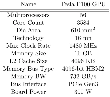
Table 4.6: The hardware specification of Tesla P100 GPU
Name Tesla P100 GPU Multiprocessors 56
Core Count 3584
Die Area 610 mm2
Technology 16 nm
Max Clock Rate 1480 MHz
Memory Size 16 GB
L2 Cache Size 4096 KB Memory Bus Type 4096-bit HBM2
Memory BW 732 GB/s
Bus Interface PCIe Gen3
Board Power 300 W
Table 4.7: The total on-chip SRAM requirement for a cluster
Bottom-up Horizontal Top-down Total Layer Weights Weights Weights Memory
(Kb) (Kb) (Kb) (Mb)
Layer 1 15000 312500 62500 381
Layer 2 62500 7500 2500 71
Layer 3 2500 625 0 4
Total 455