False Data Injection Attacks against State
Estimation in Electric Power Grids
Yao Liu, Peng Ning
Department of Computer Science
North Carolina State University
Emails:
{
yliu20, pning
}
@ncsu.edu
Michael K. Reiter
Department of Computer Science
University of North Carolina, Chapel Hill
Email: [email protected]
Abstract—A power grid is a complex system connecting electric power generators to consumers through power transmission and distribution networks across a large geographical area. System monitoring is necessary to ensure the reliable operation of power grids, and state estimation is used in system monitoring to best estimate the power grid state through analysis of meter measure-ments and power system models. Various techniques have been developed to detect and identify bad measurements, including the interacting bad measurements introduced by arbitrary, non-random causes. At first glance, it seems that these techniques can also defeat malicious measurements injected by attackers, since such malicious measurements can be considered as interacting bad measurements.
In this paper, we present a new class of attacks, called false data injection attacks, against state estimation in electric power grids. We show that an attacker can take advantage of the configuration of a power system to launch such attacks to successfully bypass the existing techniques for bad measurement detection. Moreover, we look at two realistic attack scenarios, in which the attacker is either constrained to some specific meters (due to the physical protection of the meters), or limited in the resources required to compromise meters. We show that the attacker can systematically and efficiently construct attack vectors in both scenarios, which can not only change the results of state estimation, but also modify the results in a predicted way. We demonstrate the success of these attacks through simulation using the IEEE 9-bus, 14-bus, 30-bus, 118-bus, and 300-bus systems. Our results indicate that security protection of the electric power grid must be revisited when there are potentially malicious attacks.
I. INTRODUCTION
A power grid is a complex system connecting a variety of electric power generators to customers through power trans-mission and distribution networks across a large geographical area, as illustrated in Figure 1. The security and reliability of power grids has critical impact on society and people’s daily life. For example, on August 14, 2003, a large portion of the Midwest and Northeast United States and Ontario, Canada, experienced an electric power blackout, which affected an area with a population of about 50 million people. The estimated total costs range between $4 billion and $10 billion (U.S. dollars) in the United States, and $2.3 billion (Canadian dollars) in Canada [1].
System monitoring is necessary to ensure the reliable operation of power grids. It provides pertinent information on the condition of a power grid based on the readings
Generation
Transmission
Distribution
Customers
Transmission Substation
Subtransmission Substations
Distribution Substations
Fig. 1. A power grid connecting power plants to customers via power transmission and distribution networks (revised from [2])
of meters placed at important area of the power grid. The meter measurements may include bus voltages, bus real and reactive power injections, and branch reactive power flows in every subsystem of a power grid. These measurements are typically transmitted to a control center, a component that retains crucial system data and provides centralized monitoring and control capability for the power grid. Measurements are usually stored in a telemetry system, which is also known as
Supervisory Control And Data Acquisition (SCADA) system. State estimation is used in system monitoring to best estimate
the power grid state through analysis of meter measurement data and power system models.
State estimation is the process of estimating unknown state variables in a power grid based on the meter measurements. The output of state estimation is typically used in contingency analysis, which will then be used to control the power grid components (e.g., to increase the yield of a power generator) to maintain the reliable operation even if some faults (e.g., a generator breakdown) may occur next.
online video1 that teaches people how to manipulate electric meters to cut their electricity bills. Though this meter-hacking tutorial is about meters at the end consumers, it is conceivable that attackers have the same kind of ability to modify the meters in the power grid to introduce bad measurements if they have access to these meters. If these bad measurements affect the outcome of state estimation, they can mislead the power grid control algorithms, possibly resulting in catastrophic consequences.
Power systems researchers have realized the threat of bad measurements and developed techniques for processing them (e.g., [3]–[8]). These techniques first detect if there are bad measurements, and then identify and remove the bad ones if there are any. Some of these techniques (e.g., [3], [6], [7]) were targeted at arbitrary, interacting (i.e., correlated) bad measure-ments. At first glance, it seems that these approaches can also defeat the malicious measurements injected by attackers, since such malicious measurements can be considered as interacting bad measurements.
However, in this paper, we discover that all existing tech-niques for bad measurement detection and identification can be bypassed if the attacker knows the configuration of the power system. The fundamental reason of this failure is that all existing techniques for bad measurement detection rely on the same assumption that “when bad measurements take place, the squares of differences between the observed measurements and their corresponding estimates often become significant [8].” Unfortunately, our investigation indicates that this assumption is not always true. Indeed, with the knowledge of the power system configuration, the attacker can systematically generate bad measurements so that the above assumption is violated, thus bypassing bad measurements detection.
In this paper, we present a new class of attacks, called
false data injection attacks, against state estimation in electric
power systems. By taking advantage of the configuration information of a power system, an attacker can inject malicious measurements that will mislead the state estimation process without being detected by any of the existing techniques for bad measurement detection.
State estimation uses power flow models. A power flow
model is a set of equations that depicts the energy flow on each
transmission line of a power grid. An AC power flow model is a power flow model that considers both real and reactive power and is formulated by equations that are nonlinear. For large power systems, state estimation using an AC power flow model is computationally expensive and even infeasible in many cases. Thus, power system engineers sometimes only consider the real power and use a linearized power flow model, DC
power flow model, to approximate AC power flow model [9],
[10]. A DC power flow model is less accurate, but simpler and more robust than an AC model due to the linearity [10]. In this paper, as the first step in our research, we focus on
1http://www.metacafe.com/watch/811500/electric meter hack how to
cut your electricity bill in half/
attacks against state estimation using DC power flow models. We expect the results of this paper to serve as the foundation for future research for generalized power flow models.
We present false data injection attacks from the attacker’s perspective. We first show that it is possible for the attacker to inject malicious measurements that can bypass existing techniques for bad measurement detection. We then look at two realistic attack scenarios. In the first attack scenario, the attacker is constrained to accessing some specific meters due to, for example, different physical protection of the meters. In the second attack scenario, the attacker is limited in the resources required to compromise meters. We consider two realistic attack goals: random false data injection attacks, in which the attacker aims to find any attack vector as long as it can lead to a wrong estimation of state variables, and targeted
false data injection attacks, in which the attacker aims to find
an attack vector that can inject a specific error into certain state variables. We show that the attacker can systematically and efficiently construct attack vectors for false data injection attacks in both attack scenarios with both attack goals.
We validate these attacks through simulation using the IEEE test systems, including IEEE 9-bus, 14-bus, 30-bus, 118-bus, and 300-bus systems [11]. The simulation results demonstrate the success of these attacks. For example, to inject a specific malicious value into one target state variable, the attacker only needs to compromise 10 meters in most cases in the IEEE 300-bus system, which has 1,122 meters in total.
Practical Implication: We would like to point out that the
false data injection attacks do pose strong requirements for the attackers. It requires that the attackers know the configuration of the target power system, which is in general not easy to access. Moreover, the attackers have to manipulate some meters or their measurements before they are used for state estimation. Nevertheless, it is critical for power engineers and security people to be aware of this threat. Existing state estimation and the follow-up processes such as contingency analysis assume near-perfect detection of large bad measure-ments, while our results indicate that the attackers can always bypass the detection by manipulating the measurement values. Such a discrepancy may be amplified in the later processes following state estimation and lead to catastrophic impacts, even if attackers have difficulty launching such attacks directly in real power systems.
II. PRELIMINARIES
A. Background
Power System (Power Grid): A power transmission system
(or simply a power system) consists of electric generators, transmission lines, and transformers that form an electrical network [12]. This network is also called a power grid. It connects a variety of electric generators together with a host of users across a large geographical area. Redundant paths and lines are provided so that power can be routed from any power plant to any customers, through a variety of routes, based on the economics of the transmission path and the cost of power. A control center is usually used to monitor and control the power system and devices in a geographical area.
State Estimation: Monitoring the power flows and
volt-ages in a power system is important in maintaining system reliability. To ensure that a power system continues to operate even when some components fail, power engineers use meters to monitor the system components and report their readings to the control center, which then estimates the state of power system variables from these meter measurements. Examples of state variables include bus voltage angles and magnitudes. The state estimation problem is to estimate power system state variables x = (x1, x2, ..., xn)T based on the meter measurements z = (z1, z2, ..., zm)T, where n and m are positive integers and xi, zj ∈ R for i = 1,2, ..., nand j =
1,2, ..., m[12]. More precisely, assume e= (e1, e2, ..., em)T with ej ∈ R, j = 1,2, ..., m, are measurement errors, the state variables are related to the measurements through the following model
z=h(x) +e, (1)
whereh(x) = (h1(x1, x2, ..., xn), h2(x1, x2, ..., xn), ...,
hm(x1, x2, ..., xn))T and hi(x1, x2, ..., xn) is a function of
x1, x2, ..., xn. The state estimation problem is to find an estimate ˆx of x that is the best fit of the measurement z according to Equation (1).
For state estimation using DC power flow model, Equa-tion (1) can be represented by a linear regression model
z=Hx+e, (2)
whereH= (hi,j)m×n. Three statistical estimation criteria are commonly used in state estimation: the maximum likelihood
criterion, the weighted least-square criterion, and the mini-mum variance criterion [12]. When meter error is assumed to
be normally distributed with zero mean, these criteria lead to an identical estimator with the following matrix solution
ˆ
x= (HT
WH)−1
HTWz, (3)
whereWis a diagonal matrix whose elements are reciprocals
of the variances of meter errors. That is,
W=
σ−12 σ−2
2
· ·
σ−2 m
, (4)
whereσ2
i the variance of thei-th meter (1≤i≤m). Bad Measurement Detection: Bad measurements may be
introduced due to various reasons such as meter failures and malicious attacks. Techniques for bad measurements detection have been developed to protect state estimation [3], [12]. Intuitively, normal sensor measurements usually give an es-timate of the state variables close to their actual values, while abnormal ones may “move” the estimated state variables away from their true values. Thus, there is usually “inconsistency” among the good and the bad measurements. Power systems researchers proposed to calculate the measurement residual z−Hˆx (i.e., the difference between the vector of observed measurements and the vector of estimated measurements), and use its L2-norm kz−Hˆxk to detect the presence of bad
measurements. Specifically, kz−Hˆxk is compared with a thresholdτ, and the presence of bad measurements is assumed ifkz−Hˆxk> τ.
The selection ofτ is a key issue. Assume that all the state variables are mutually independent and the meter errors follow the normal distribution. It can be mathematically shown that kz−Hˆxk2, denotedL(x), follows aχ2(v)-distribution, where v=m−nis the degree of freedom. According to [12],τ can be determined through a hypothesis test with a significance level α. In other words, the probability that L(x) ≥ τ2 is
equal to α. Thus, L(x) ≥ τ2 indicates the presence of bad
measurements, with the probability of a false alarm beingα.
B. Related Work
Many researchers have considered the problem of bad mea-surements detection and identification in power systems [4]. Early power system researchers realized the existence of bad measurements and observed that a bad measurement usually led to large normalized measurement residual. After the presence of bad measurements is detected, they mark the measurement having the largest normalized residual as the suspect and remove it [5], [13]–[19]. For example, Schweppe et al. [13] filter one measurement having the largest normalized residual at each loop, and then rerun the same process on the reduced measurement set until the detection test is passed. Handschin et al. [14] proposed a grouped residual search strategy that can remove all suspected bad measurements at the same time.
bad measurements. The largest normalized residual method
does not work satisfactorily in dealing with interacting bad measurements. To address this problem, Hypothesis Testing Identification (HTI) [7] and Combinatorial Optimization Iden-tification (COI) [6], [20], [21] were developed. HTI selects a set of suspected bad measurements according to their normalized residuals, and then decide whether an individual suspected measurement is good or bad through hypothesis testing. COI uses the framework from the decision theory to identify multiple interacting bad measurements. For example, Asada et al. [20] proposed an intelligent bad data identification strategy based on tabu search to deal with multiple interacting bad measurements.
Recently, the focus in bad measurement processing is on the improvement of the robustness using phasor measurement units (PMUs) [22]–[25]. For example, Chen et al. [22] used PMUs to transform the critical measurements into redundant measurements such that the bad measurements can be detected by the measurement residual testing and the system is still observable.
At first glance, it seems that these approaches can also defeat the malicious measurements injected by attackers, since such malicious measurements can be considered as interacting bad measurements. However, in this paper, we show that an attacker can systematically bypass the detection of all these approaches.
III. FALSEDATAINJECTIONATTACKS
We assume that there are m meters that provide m mea-surements z1, ..., zm. We also assume that there are n state variables x1, ..., xn. The relationship between these m meter measurements and n state variables can be characterized by anm×nmatrixH, as discussed in Section II. In general, the matrix H of a power system is a constant matrix determined by the topology and line impedances of the system. How the control center constructs His illustrated in [3].
We assume that the attacker knows the matrix H of the target power system. For example, the attacker can obtain H by intruding into the control center of the target system. The attacker generates malicious measurements based on the matrix H, and then injects the malicious measurements into the compromised meters to undermine the state estimation process. The injected malicious measurements can introduce arbitrary errors into the output of state estimation without being detected by the existing approaches.
As discussed earlier, we consider two realistic attack goals:
random false data injection attacks, in which the attacker aims
to find any attack vector as long as it can result in a wrong estimation of state variables, and targeted false data injection
attacks, in which the attacker aims to find an attack vector that
can inject a specific error into certain state variables.
We use the following two realistic attack scenarios to facilitate the discussion on how the attacker can construct attack vectors to bypass the current bad measurement detection
scheme. Note, however, that the false data injection attacks are not constrained by these attack scenarios.
• Scenario I – Limited Access to Meters: The attacker is restricted to accessing some specific meters due to, for example, different physical protection of meters. • Scenario II – Limited Resources to Compromise
Meters: The attacker is limited in the resources required
to compromise meters. For example, the attacker only has resources to compromise up tok meters. Due to the limited resources, the attacker may also want to minimize the number of meters that have to be compromised in order to launch a false data injection attack.
In the following, we first show the basic principle of false data injection attacks. We then focus on the two attack sce-narios and show how the attacker can construct attack vectors for both random and targeted false data injection attacks.
A. Basic Principle of False Data Injection Attacks
Let za represent the vector of observed measurements that may contain malicious data. za can be represented as za=z+a, wherez= (z1, ..., zm)T is the vector of original measurements anda= (a1, ..., am)T is the malicious data that the attacker adds to the original measurements. We refer toa as an attack vector. Thei-th elementaibeing non-zero means that the attacker compromises thei-th meter, and then replaces its original measurementziwith a phony measurementzi+ai.
The attacker can choose any non-zero arbitrary vector as the attack vectora, and then construct the malicious measurements za=z+a. Letxbadˆ andxˆdenote the estimates of xusing the malicious measurementszaand the original measurements z, respectively.ˆxbadcan be represented asˆx+c, wherecis a non-zero vector of lengthn. Note thatcreflects the estimation error injected by the attacker.
As discussed in Section II, the bad measurement detec-tion algorithm computes the L2-norm of the corresponding
measurement residual to check whether there exist bad mea-surements or not. However, if the attacker can use Hc as the attack vector a (i.e., a=Hc), then the L2-norm of the
measurement residual ofzais equal to that ofz, as shown in Theorem 1. In other words, if the attacker can choosea as a linear combination of the column vectors ofH,za can pass the detection as long as zcan pass the detection.
Theorem 1: Suppose the original measurementszcan pass the bad measurement detection. The malicious measurements za=z+acan pass the bad measurement detection if a is a linear combination of the column vectors ofH(i.e.,a=Hc).
Proof: Sincezcan pass the detection, we havekz−Hˆxk ≤
of the measurement residual is
kza−Hˆxbadk = kz+a−H(ˆx+c)k = kz−Hˆx+ (a−Hc)k
= kz−Hˆxk ≤τ. (5)
Thus, the L2-norm of the measurement residual ofza is less
than the thresholdτ. This means thatzacan also pass the bad
measurement detection.
In this paper, we refer to an attack in which the attack vector aequalsHc, wherecis an arbitrary non-zero vector, as a false
data injection attack. By launching false data injection attacks,
the attacker can manipulate the injected false data to bypass the bad measurement detection and also introduce large errors into the output of the state estimation, since each element of ccould be an arbitrarily large number.
B. Scenario I – Limited Access to Meters
We assume that the attacker has access tokspecific meters. Assume Im = {i1, ..., ik} is the set of indices of those meters. In other words, the attacker can modify zij, where
ij∈ Im. To launch a false data injection attack without being detected, the attacker needs to find a non-zero attack vector a= (a1, ..., am)T such thatai= 0fori /∈ Imandais a linear combination of the column vectors ofH (i.e.,a=Hc).
We now present random and targeted false data injection attacks, respectively.
1) Random False Data Injection Attack: As discussed
earlier, the non-zero attack vector a satisfies the condition a= (a1, ..., am)T =Hcwithai= 0fori /∈ Im. In a random false data injection attack, the vector c (i.e., the estimation errors introduced to the state variables) can be any value.
The attacker can find an attack vector a as follows. First, the attacker can compute an equivalent form of the rela-tion a=Hc by eliminating c. To simplify the notation, let
P=H(HT
H)−1
HT
, andB=P−I. It is easy to see that PH=H. The attacker can simply multiplyPto both sides of the relationa=Hcto obtain a sequence of equivalent forms, as shown below:
a=Hc ⇔ Pa=PHc⇔Pa=Hc⇔Pa=a
⇔ Pa−a=0⇔(P−I)a=0
⇔ Ba=0. (6)
This means that a vector a satisfies the relation a=Hc if and only if it satisfies the relation Ba=0. So the attacker needs to find a non-zero attack vector a such that Ba=0 andai= 0 fori /∈ Im.
There are many known approaches for obtaining attack vectors from the above equation. Here we give a simple one. The attacker can represent a as a = (0, ...,0, ai1,0, ...,0, ai2,0, ...,0, aik,0, ...,0)
T,
where ai1, ai2, ..., aik are the unknown variables to
be solved. Suppose B = (b1, ...,bm), where bi (1 ≤ i ≤ m) is the i-th column vector of B. Thus,
Ba= 0⇔(...,bi1, ...,bi2, ...,bik, ...)(0, ...,0, ai1,0, ...,0, ai2,0, ...,0, aik,0, ...,0)
T = 0. Let the m × k
matrix B′ = (b
i1, ...,bik) and the length k vector
a′
= (ai1, ..., aik)
T. We have
Ba=0⇔B′a′ =0.
If the rank of B′ is less than k, B′ is a rank deficient matrix, and there exist infinite number of non-zero solutions
a′
that satisfy the relationB′a′
=0[26]. According to [26], the solution isa′ = (I−B′−B)d, whereB′−is the Matrix-1 inverse ofB′ anddis an arbitrary non-zero vector of length
k. With a non-zero solutiona′, the attacker can construct the corresponding attack vectora by filling 0’s as the remaining elements ina.
If the rank of B′ is equal to k, then B′ is not a rank deficient matrix and the relation B′a′=0 has a unique solutiona′ =0[26]. This meansa=0. As a result, no error can be injected into the state estimation, and the attacker vector does not exist.
It is possible that the attack vector does not exist if k is too small. However, if k ≥ m−n+ 1, the attack vector always exists, as shown in Theorem 2. Moreover, as long as the attacker can compromisem−n+ 1or more meters, the attacker can always successfully construct an attack vector to bypass the detection.
Theorem 2: If the attacker can compromisekspecific me-ters, where k≥m−n+ 1, there always exist attack vectors a=Hc such thata6=0andai= 0fori /∈ Im.
Proof: According to Equation (6),a=Hc⇔Ba=0, where
B=P−I=H(HT
H)−1
HT−I.Hshould be anm×nfull rank matrix to allow the estimation ofxfromz[12]. Without loss of generality, we further assumem≥n. Thus, rank(H) =
n.Pis a projection matrix ofH, sinceP=H(HT
H)−1
HT
. Thus, rank(P) =rank(H) =n, and n eigenvalues of Pare 1’s and the remainingm−n eigenvalues of Pare 0’s [26]. Obviously, forB=P−I,m−neigenvalues ofBare 1’s and
neigenvalues ofBare 0’s. Therefore, rank(B) =m−n. The matrixB′ is am×k matrix. So rank(B′)≤m−n. Further consideringk≥m−n+ 1, we have rank(B′)< k. Thus,B′ is rank deficient matrix and there exist infinite number of non-zero solutions for a′ that satisfy the relation B′a′ =0. This means there exist many non-zero attack vectors a in which
ai= 0 fori /∈ Im.
Indeed, when k≥m−n+ 1, the attacker does not need to compute the matrices B and B′ to solve the equation
B′
a′
= 0. Instead, the attacker can use an alternative algo-rithm based on elementary matrix transformation to directly construct attack vectors. Intuitively, the attacker can perform column transformations onHsuch that some column vectors in the resulting matrix become linear combinations of column vectors inHand at the same time, the elements corresponding to the meters not controlled by the attacker are eliminated (i.e.,
Let I¯m = {j|1 ≤ j ≤ m, j /∈ Im}. It is easy to see that the size of I¯m is m−k, since the size ofIm isk. Let
H= (h1, ...,hn), wherehi = (h1,i, ..., hm,i)T for1≤i≤n. For a random j ∈ I¯m, the attacker first scans the matrix H to find a column vector whose j-th element is not zero. If the attacker can find such a vector, the attacker swaps it with the first column vector h1. Then, the attacker can construct
anm×(n−1)matrixH1= (h1
1, ...,h
1
n−1)by performing
column transformations on Has shown below:
h1i=
(
h1−hj,ihj,1
+1hi+1, ifhj,i+1 6= 0,1≤i≤n−1
hi+1, ifhj,i+1 = 0,1≤i≤n−1
(7)
If the j-th element is zero for all the column vectors of H, then h1
i =hi for1 ≤ i ≤n−1. As a result, thej-th row of H1
are all zeros. The attacker repeats this process to the reduced matrix H1 and the reduced matrices thereafter using a different element inI¯m, until all elements inI¯m are exhausted. Finally, the attacker can get a matrix having at least one column vector, since m−k ≤ n−1. Obviously, the column vectors of the final matrix are linear combinations of the column vectors of H, and them−k rows with index
j ∈I¯m of this matrix consist of all 0’s. Any column vector can be used as an attacker vector.
2) Targeted False Data Injection Attack: In a targeted false
data injection attack, the attacker intends to inject specific errors into the estimation of certain chosen state variables. This attack can be represented mathematically as follows. Let Iv={i1, ..., ir}, wherer < n, denote the set of indexes of the
rtarget state variables chosen by the attacker. In other words, the attacker has chosen xi1, xi2, ..., xir as the target state
variables. In this attack, the attacker intends to construct an attack vectorasuch that the resulting estimateˆxbad=ˆx+c, where c= (c1, c2, ..., cn)T and ci fori ∈ Iv is the specific error that the attacker has chosen to inject to xˆi. That is, the attacker wants to replace xˆi1, ..., and xˆir with xˆi1 +ci1, ...,
andxˆir+cir, respectively.
We consider two cases for the targeted false data injection attack: A constrained and an unconstrained case. In the con-strained case, the attacker wants to launch a targeted false data injection attack that only changes the target state variables but does not pollute the other state variables. The constrained case represents the situations where the control center (software or operator) may know or have ways to verify the estimates of the other state variables. In the unconstrained case, the attacker has no concerns on the impact on the other state variables when attacking the chosen ones.
The construction of an attack vector a becomes rather simple in the constrained case. Consider the relationa=Hc. As discussed earlier, the attack vector a must satisfy the condition that ai= 0 wherei /∈ Im. Note that every element
ci incis fixed, which is either the chosen value wheni∈ Iv or 0 when i /∈ Iv. Thus, the attacker can substitute c back into the relation a=Hc, and check if ai = 0 for ∀i /∈ Im. If yes, the attacker succeeds in constructing the (only) attack vector a. Otherwise, the attack is impossible.
Now let us consider the unconstrained case. In this case, only the elements ci of c for i ∈ Iv are fixed; the other elementscjforj /∈ Ivcan be any values. The attacker can use an approach similar to the one for random false data injection attacks to construct an attack vector. Specifically, the attacker can first transform a=Hc into an equivalent form without havingc, and then solvea from the equivalent form.
Note that a = Hc = P
i /∈Ivhici +
P
j∈Ivhjcj. Let Hs = (hj1, ...,hjn−r) and cs = (cj1, ..., cjn−r)
T, where
ji ∈ I/ v for 1 ≤ i ≤ n−r. Further let b = Pj∈Ivhjcj,
Ps=Hs(HT
s Hs) −1
HT
s,Bs =Ps−I, andy=Bsb. Thus, the relation a = Hc can be transformed into the following equivalent forms
a=Hc ⇔ a= X
i /∈Iv
hici+
X
j∈Iv
hjcj=Hscs+b
⇔ Psa=PsHscs+Psb
⇔ Psa=Hscs+Psb ⇔ Psa=a−b+Psb ⇔ (Ps−I)a= (Ps−I)b
⇔ Bsa=Bsb⇔Bsa=y (8)
This implies thatasatisfies the relationa=Hcif and only if a satisfies the relationBsa=y. (It is easy to see that Bs is anm×mmatrix.) Thus, the attacker needs to find an attack vectora such thatBsa=ywherea= (a1, a2, ..., am)T and
ai= 0 fori /∈ Im.
There are k unknown elements in a at positions i1, ..., ik, where i1, ..., ik ∈ Im. Thus, the vector a can be written as a = (0, ...,0, ai1,0, ...,0, ai2,0, ...,0, aik,0, ...,0)
T, where
aij’s are unknown elements that need to be solved. Suppose
Bs = (bs1, ...,bsm), where bsi (1 ≤ i ≤ m) is the
i-th column vector of Bs. We follow the same reasoning as in Section III-B1 to denote B′
s = (bsi1, ...,bsik) and
a′ = (a
i1, ..., aik)
T. Then we have
B′sa′=y⇔Bsa=y⇔a=Hc.
Thus, to construct an attack vector, the attacker needs to check if the rank of B′s is the same as the rank of the augmented matrix (B′
s|y). If yes, the relation B′sa′=y is a consistent equation. According to [26], there exist infinite number of solutionsa′=B′−s y+ (I−B
′−
s Bs)dthat satisfy the relationB′sa′=y, where B′−
s is the Matrix-1 inverse of
B′
s and d is an arbitrary non-zero vector of length k. The attacker can construct an attack vectora from anya′
6=0. If the rank ofB′s is not the same as the rank of the augmented matrix(B′s|y), then the relationB′sa′=yis not a consistent equation, and thus has no solution. This means that the attacker cannot construct an attack vector to inject the specific errors into the chosen state variables.
C. Scenario II – Limited Resources to Compromise Meters
of presentation, we call a length-mvector ak-sparse vector if
it has at most k non-zero elements. Thus, the attacker needs to find a k-sparse, non-zero attack vectora that satisfies the relationa=Hc.
As in Scenario I, we consider both random and targeted false data injection attacks in Scenario II.
1) Random False Data Injection Attack: With the resources
to compromise up to k meters, the attacker may use a brute-force approach to construct an attack vector. That is, the attacker may try all possible a’s consisting of k unknown elements and m−k zero elements. For each candidate a, the attacker may check if there exists a non-zero solution of a such that Ba=0using the same method as discussed in Section III-B1. If yes, the attacker succeeds in constructing an attack vector. If the attacker cannot find a k-sparse attack vector after exhausting all the possible a’s, the attack vector does not exist. However, the brute-force approach could be time consuming. In the worst case, the attacker needs to examine mk
candidate attack vectors.
To improve the time efficiency, the attacker may take ad-vantage of the following observation. Since a successful attack vector is a linear combination of the column vectors ofH(i.e., a=Hc), the attacker can perform column transformations to Hto reduce the non-zero elements in the transformed column vectors. As this process continues, more column vectors in the transformed H will have fewer non-zero elements. The column vectors with no more than k non-zero elements can be used as attack vectors. In particular, when the matrix H is a sparse matrix (which is usually the case in real power systems), it does not take many column transformations to construct a desirable attack vector.
We give a heuristic approach to take advantage of this observation as follows. The attacker can initialize a size n
queue with the n column vectors of H. The attacker then repeats the following process: Take the first column vectort out from the queue. If t is a k-sparse vector, the algorithm returns andtcan be used as the attack vector. If not, for each column vector sin the queue, the attacker checks if linearly combining t and s can result in a column vector with less zero elements thant. If so, the attacker appends the resulting vector into the queue. The attacker repeats this process until a
k-sparse vector is found or the set is empty. It is easy to see that ak-sparse vector constructed in this way must be a linear combination of some column vectors of H, and can serve as an attack vector.
The heuristic approach could be quite slow for a general H. However, it works pretty efficiently for a sparse matrixH, which is usually the case for real-world power systems. For example, in our simulation, whenk= 12in the IEEE 300-bus test system, it takes the heuristic approach about 16.63 seconds on a regular PC to find an attack vector after computing 596 linear combinations of column vectors. As another example, when k = 6 in the IEEE 118-bus test system, it takes this approach about 5.82 seconds to find an attack vector after 900 linear combinations of column vectors.
The heuristic approach does not guarantee the construction of an attack vector even if it exists, nor does it guarantee the construction of an attack vector that has the minimum number of non-zero elements. Nevertheless, it runs pretty quickly when it can construct an attack vector, and thus could still be a useful tool for the attacker.
Ideally, in order to reduce the attack costs, the attacker would like to compromise as few meters as possible. In other words, the attacker wants to find the optimal attack vectora with the minimum number of non-zero elements. The attacker may use the brute-force approach discussed at the beginning of Section III-C1 withkbeing 1 initially, and gradually increase
k until an attack vector is found. Apparently, such an attack vector gives the optimal solution with the minimum number of compromised meters. There are possibilities to improve such a brute-force approach, for example, using a binary search in identifying the minimumk.
2) Targeted False Data Injection Attack: We follow the
notation used in Scenario I to describe the targeted false data injection attack. Let Iv = {i1, ..., ir}, where r < n, denote the set of indexes of the r target state variables chosen by the attacker. In this attack, the attacker intends to construct an attack vectora to replace xˆi1, ..., and xˆir withxˆi1+ci1, ...,
and ˆxir +cir, respectively, whereci1, ..., cir are the specific
errors to be injected.
Similar to Scenario I, we consider both constrained and unconstrained cases. As discussed earlier, in the constrained case, the attacker intends to only change the estimation of the chosen target state variables, but does not modify the other state variables. Thus, all elements of c are fixed. So the attacker can substitute c into the relation a=Hc. If the resulting a is ak-sparse vector, the attacker succeeds in constructing the attack vector. Otherwise, the attacker fails. The attack vector derived in the constrained case is the only possible attack vector; there is no way to further reduce the number of compromised meters.
Now let us consider the unconstrained case. Only the elements ci of c for i ∈ Iv are fixed; the other elements
cj forj /∈ Iv can be any values. According to Equation (8),
a=Hc⇔Bsa=y. (Note that the derivation of Equation (8) does not assume any specific compromised meters. Thus, Equation (8) also holds in the unconstrained case in Scenario II.)
To construct an attack vector, the attacker needs to find a
k-sparse attack vector a that satisfies the relation Bsa=y. A closer look at this problem reveals that it is the Minimum
Weight Solution for Linear Equations problem [27], which is
an NP-Complete problem: Given a matrixAand a vectorb, compute a vectorxsatisfyingAx=bsuch thatxhas at most
knon-zero elements.
In our simulation, we choose to use the Matching Pursuit algorithm, since it is the most popular algorithm for computing the sparse signal representations and has exponential rate of convergence [34].
The attacker may also want to minimize the number of meters to be compromised. That is, the attacker needs to find an attack vector a with the minimum number of non-zero elements that satisfies a=Hc such that the chosen elements inchave the specific values. This problem is in fact the MIN RVLS= problem [35]: Given a matrix A and a vector b,
compute a vectorxsatisfyingAx=bsuch thatxhas as few non-zero elements as possible. Matching Pursuit Algorithm can again be used to find an attack vector, since this problem is the optimization version of the minimum weight solution for linear equations problem discussed earlier.
D. Discussion
We would like to point out that the false data injection attacks do pose strong requirements for the attackers. In particular, it requires that the attackers know the configuration of the target power system. Such information is usually kept secret by power companies at control centers or other places with physical security measures. Thus, it is non-trivial for the attackers to obtain the system configuration information to launch these attacks. Nevertheless, it would be definitely wrong to assume that the attackers cannot access such infor-mation at all. As pointed out in [2], an attacker may break into the control center through four interfaces. Moreover, the attackers may pursue social engineering approaches to get such information.
Another challenge for the attackers is the manipulation of the meter measurements. The attackers may physically tamper the meters, or manipulate the meter measurements before they are used for state estimation in the control center. Again, due the existing protection in the power grid, this is non-trivial. However, assuming that this is impossible will definitely give us a false sense of security and will pave ways for catastrophes in the future.
Despite the difficulty for launching false data injection attacks, it is critical for power engineers and security people to be aware of this threat. Existing state estimation and the follow-up processes assume a near-perfect detection of large bad measurements. However, our work in this paper indicates that an attacker can systematically bypass detection. This discrepancy may be amplified in the later processes following state estimation, leading to catastrophic impacts. Additional research is necessary to clarify the implication of the false data injection attacks.
IV. EXPERIMENTALRESULTS
In this section, we validate the false data injection attacks through experiments using IEEE test systems, including the IEEE 9-bus, 14-bus, 30-bus, 118-bus, and 300-bus systems. We are primarily interested in assessing the feasibility of
constructing attack vectors in various situations as well as the efforts required for a successful attack vector construction.
In our experiments, we simulate attacks against state es-timation using DC power flow model. We extract the con-figuration of the IEEE test systems (particularly the matrix H) from MATPOWER, a MATLAB package for solving power flow problems [11]2. We perform our experiments based
on the matrix H and meter measurements obtained from MATPOWER. For each test system, the state variables are voltage angles of all buses, and the meter measurements are real power injections of all buses and real power flows of all branches. We simulate the behavior of compromising thei-th meter by adding an offset (chosen by the attack) to the i-th measurement.
The numbers of state variables and measurements for all the test systems and some examples of matrix H are given in Appendix A. Other information (such as the topology, the locations of meters, bus data, and branch data) can be found in the source files in MATPOWER.
All the experiments are simulated in MATLAB 7.4.0 on a DELL PC running Windows XP, which has a 3.0 GHz Pentium 4 processor and 1 GB memory.
A. Results of Scenario I
As mentioned earlier, in Scenario I, the attacker is limited to accessing k specific meters. In other words, the attacker can only modify the measurements of these k meters. Our evaluation objective in this scenario is mainly two-fold. First, we would like to see how likely the attacker can use these
k meters to achieve his/her attack goal. Second, we want to see the computational efforts required for finding an attack vector. In our evaluation, we consider (1) random false data injection attacks, (2) targeted false data injection attacks in the unconstrained case, and (3) targeted false data injection attacks in the constrained case.
Based on our evaluation objective, we use two evaluation metrics. The first metric is the probability that the attacker can successfully construct an attack vector given thekspecific meters. The second metric is the execution time required to either construct an attack vector or conclude that the attack is infeasible.
We perform the experiments as follows. For random false data injection attacks, we let the parameter k range from 1 to the maximum number of meters in each test system. (For example,kranges from 1 to 490 in the IEEE 118-bus system.) For each k, we randomly choose k specific meters and use the approach presented in Section III-B1 to attempt an attack vector construction. We repeat this process 100 times for both IEEE 118-bus and 300-bus systems and 1,000 times for the other systems3, and estimate the success probability p
k (i.e.,
2In MATPOWER, the shift injection vector is set to0for state estimation
using DC power flow model.
3It takes significantly more time to exhaustively examine the IEEE
118-bus and 300-118-bus systems with all possiblek’s. Thus, we reduce the number
the probability of successfully constructing an attack vector withk given meters) aspk= #successf ul trails#trials .
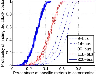
Let Rk denote the percentage of the specific meters under attacker’s control (i.e.,total number of metersk ). Figure 2 shows the relationship between pk and Rk for random false data injection attacks. We can see thatpk increases sharply asRk is larger than a certain value in all systems. For example,pk of the IEEE 300-bus system increases quickly whenRk exceeds 20%. Moreover, the attacker can generate the attack vector with the probability close to 1 when Rk is large enough. For example, pk is almost 1 when Rk is greater than 60% and 40% in the IEEE 118-bus and 300-bus systems, respectively. Finally, larger systems have higherpkthan smaller systems for the same Rk. For example,pk is about 0.6 for IEEE 300-bus system and 0.1 for IEEE 118-bus system when the attacker can compromise 30% of the meters in both systems.
0 0.2 0.4 0.6 0.8 1
0 0.2 0.4 0.6 0.8 1
Percentage of specific meters to compromise
Probability of finding the attack vector
9−bus 14−bus 30−bus 118−bus 300−bus
Fig. 2. Probability of finding an attack vector for random false data injection attacks
0 0.2 0.4 0.6 0.8 1
0 0.2 0.4 0.6 0.8 1
Percentage of specific meters to compromise
Probability of finding the attack vector
9−bus 14−bus 30−bus 118−bus 300−bus
Fig. 3. Probability of finding an attack vector for compromising a single state variable in targeted false data injection attacks (unconstrained case)
For targeted false data injection attacks in the unconstrained case, we also let the parameter k range from 1 to the maximum number of meters in each test system, and perform the following experiments for each k. We randomly pick 10 target state variables for each test system (8 for the IEEE 9-bus system, since it only has 8 state variables). For each target state variable, we perform multiple trials (1,000 trials for the IEEE 9-bus, 14-bus, and 30-bus systems, 100 trials for the IEEE
118-bus system, and 20 trials for the IEEE 300-118-bus system)4. In each trail, we randomly choosekmeters and test if an attack vector that injects false data into this target variable can be generated. If yes, we mark the experiment as successful. After these trails, we can compute the success probability pk,v for this particular state variable v as pk,v = #successf ul trails#trials . Finally, we compute the overall success probabilitypk as the average ofpk,v’s for all the chosen state variables.
Figure 3 shows the relationship between pk and Rk for targeted false data injection attacks in the unconstrained case. We observe the same trend in this figure as in Figure 2, though the probability in this case is in general lower than that in Figure 2. For example, pk increases sharply as Rk is larger than 60% for both the IEEE 118-bus and 300-bus systems. Moreover, for both systems, the probability that the attacker can successfully generate the attack vector is larger than 0.6 whenRk is larger than 70%. For targeted false data injection attacks, larger systems also tend to have higherpkthan smaller systems for the same Rk.
Figures 2 and 3 indicate that it is possible for the attacker to successfully generate attack vectors in the above two attacks, even if the attacker has limited access to some specific meters. The success probability increases dramatically as the number of meters controlled by the attacker increases beyond a threshold.
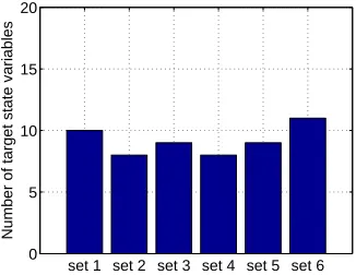
The targeted false data injection attack in the constrained case is the most challenging one for the attacker. Due to the constraints on the specific meters, the targeted state variables, and the necessity of no impact on the remaining state variables, the probability of constructing a successful attack vector is in fact very small, though still possible. We perform experiments for this case slightly differently. We randomly pick 6 sets of meters for the IEEE 118-bus and 300-bus systems. In each set, there are 350 meters and 700 meters for the IEEE 118-bus and 300-bus systems, respectively. We then check the number of individual target state variables that can be affected by each set of meters in the constrained case (i.e., without affecting the estimation of the remaining state variables).
Figures 4 and 5 show the impact of targeted false data injection attacks in the constrained case. The attacker can affect 8–11 individual state variables in the IEEE 118-bus system and 13–16 individual state variables in the IEEE 300-bus system. Thus, though the targeted false data injection attack in the constrained case is hard, it is still possible to modify some target state variables.
In Scenario I, all attacks can be performed fairly quickly. In other words, it takes little time for the attacker to know if it is possible to construct an attack vector. Moreover, when the attack is feasible, it takes again little time to actually construct an attack vector. Table I shows the execution time required by
4In this case, it take even more time than random false data injection
attacks to exhaustively examine the IEEE 118-bus and 300-bus systems with all possiblek’s. Thus, we reduce the number of trials for these two systems to
set 1 set 2 set 3 set 4 set 5 set 6 0
5 10 15 20
Number of target state variables
Fig. 4. Number of target state variables affected (IEEE 118-bus system)
set 1 set 2 set 3 set 4 set 5 set 6 0
5 10 15 20
Number of target state variables
Fig. 5. Number of target state variables affected (IEEE 300-bus system)
the random false data injection attack and the targeted false data injection attack in the unconstrained case. For example, the time needed for the random false data injection attack to either construct an attack vector or conclude the infeasibility of the attack ranges from 0.34ms to 867.9 ms for the 118-bus system. The time required for the targeted false data injection attack in the constrained case is very small, since the computational task is just the multiplication of a matrix and a column vector. For example, the time required for the IEEE 300-bus system ranges from 1.2ms to 11ms. We do not give the specific numbers in this paper.
B. Results of Scenario II
As mentioned earlier, in Scenario II, the attacker has limited resources to compromise up to k meters. Compared with Scenario I, the restriction on the attacker is relaxed in the sense that anyk meters can be used for the attack. Similar to Scenario I, we would also like to see how likely the attacker
TABLE I
TIMING RESULTS INSCENARIOI (MS)
Test system Random attack Targeted attack (unconstrained) IEEE 9-bus 0.17–2.4 0.21–2.2 IEEE 14-bus 0.16–5.6 0.26–11.3 IEEE 30-bus 0.35–14.9 0.24–31.4 IEEE 118-bus 0.34–867.9 0.42–1,874.5 IEEE 300-bus 0.55–8,549.6 0.73–18,510
TABLE II
RESULTS OF RANDOM FALSE DATA INJECTION ATTACKS
Test system # meters to compromise IEEE 9-bus 4 IEEE 14-bus 4 IEEE 30-bus 4 IEEE 118-bus 4 IEEE 300-bus 4
can use the limited resources to achieve his/her attack goal, and at the same time, examine the computation required for attacks. We use two evaluation metrics in our experiments: (1) number of meters to compromise in order to construct an attack vector, and (2) execution time required for constructing an attack vector.
Due to the flexibility for the attacker to choose different me-ters to compromise in Scenario II, the evaluation of Scenario II generally requires more experiments to obtain the evaluation results. In the following, we examine (1) random false data injection attacks, (2) targeted false data injection attacks in the constrained case, and (3) targeted false data injection attacks in the unconstrained case, respectively.
1) Results of Random False Data Injection Attacks:
Ran-dom false data injection attacks are the easiest one among the three types of attacks under evaluation, mainly due to the least constraints that the attacker has to follow. We perform a set of experiments to construct attack vectors for random false data injection attacks against the IEEE 9-bus, 14-bus, 30-bus, 118-bus, and 300-bus systems. We assume the attacker wants to minimize the attack cost by compromising as few meters as possible. This means the attacker needs to find the attack vector having the minimum number of non-zero elements. The brute-force approach is too expensive to use for finding such an attack vector because of its high time complexity. For example, it needs to examine about 227 combinations for the IEEE
9-bus test system. Thus, in our experiment, we use the heuristic algorithm discussed in Section III-C1 to find an attack vector that has near minimum number of non-zero elements for each system.
2) Results of Targeted False Data Injection Attacks in Constrained Case: Similar to Scenario I, targeted false data
in-jection attacks in the constrained case are the most challenging one among the three types of attacks due to all the constraints that the attacker has to follow in attack vector construction. In the constrained case, the attacker aims to change specific state variables to specific values and keep the remaining state variables as they are.
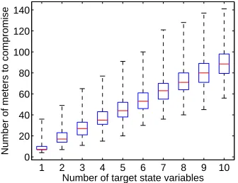
In our experiments, we randomly choose l (1 ≤ l ≤ 10) target state variables and generate malicious data for each of them. The malicious values are set to be 100 times larger than the real estimates of the state variables. We then examine how many meters need to be compromised in order to inject the malicious data (without changing the other non-target state variables). For each value of l, we perform the above experiment 1,000 times to examine the distribution of the number of meters that need to be compromised.
1 2 3 4 5 6 7 8 9 10
0 50 100 150
Number of meters to compromise
Number of target state variables
Fig. 6. Constrained case: Number of meters to compromise to inject false data intolstate variables in the IEEE 118-bus system
1 2 3 4 5 6 7 8 9 10
0 20 40 60 80 100 120 140
Number of meters to compromise
Number of target state variables
Fig. 7. Constrained case: Number of meters to compromise to inject false data intolstate variables in the IEEE 300-bus system
Figures 6 and 7 show the results for the IEEE 118-bus and 300-bus systems, respectively. In these figures, we use box plots5 to show the relationship between the number of target
5In a box plot [36], each box describes a group of data through their five
summaries: minimum, first quartile, median, third quartile, and maximum. They are represented as horizontal lines at the very bottom, at the lower end of the box, inside the box, at the upper end of the box, and at the very top, respectively.
300−bus 118−bus 30−bus 14−bus 9−bus 5
10 15 20 25 30 35
Number of meters to compromise
IEEE test systems
Fig. 8. Constrained case: Number of meters to compromise to inject false data into a single state variable
state variables and the number of meters to compromise. In the worst case, to inject malicious data into as many as 10 state variables, the attacker needs to compromise 60–140 meters in the IEEE 118-bus system and 50–140 meters in the IEEE 300-bus system. Note that there are 1,122 meters in the IEEE 300-bus system and 490 meters in the IEEE 118-bus system. This means that the attacker only needs to compromise a small fraction of the meters to launch targeted false data injection attacks even in the constrained case.
We also exhaustively examine a special situation of targeted false data injection attacks in the constrained case. Specifically, for each state variable, we examine the number of meters that need be compromised if the attacker aims at this variable. Figure 8 shows the results. We can see that the attacker can inject malicious data into any single state variable using less than 35 meters for the IEEE 118-bus system and less than 40 meters for the IEEE 300-bus system. For all the systems, none of the median values is greater than 10. This means that the attacker can affect most of the state variables by using at most 10 compromised meters.
In the constrained case, since cis fixed, the attack vectors can be directly computed. Thus, the execution time in all the experiments is very short. For example, it costs only 1.2 ms on the test computer to generate an attack vector that injects false data into 10 state variables in the IEEE 300-bus system.
3) Results of Targeted False Data Injection Attacks in Unconstrained Case: In the unconstrained case, the attacker
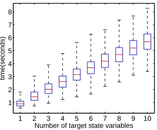
wants to inject malicious data into specific state variables, but the attacker does not have to keep the other state variables un-changed. As discussed in Section III-C2, we use the Matching Pursuit algorithm [28]–[30] to find attack vectors. We perform the same set of experiments as in Section IV-B2 to obtain the two evaluation metrics: the number of meters to compromise and the execution time. Note that in the unconstrained case, it takes significantly more time to find a near minimum number of meters than the previous experiments. Thus, we show more detailed results on execution time in this case.
systems, respectively. Figures 11 and 12 show the correspond-ing execution time of the Matchcorrespond-ing Pursuit algorithm for finding an attack vector successfully. From these figures, we can see that the attacker needs to compromise 60–130 meters for the IEEE 118-bus system and 55–140 meters for the IEEE 300-bus system, if the attacker wants to inject malicious data into as many as 10 state variables. These meters can be quickly identified within 2 seconds for the IEEE 118-bus system and within 8 seconds for the IEEE 300-bus system.
1 2 3 4 5 6 7 8 9 10
0 20 40 60 80 100 120
Number of meters to compromise
Number of target state variables
Fig. 9. Unconstrained case: Number of meters to compromise to inject false data intolstate variables in the IEEE 118-bus system
1 2 3 4 5 6 7 8 9 10
0 50 100 150
Number of meters to compromise
Number of target state variables
Fig. 10. Unconstrained case: Number of meters to compromise to inject false data intolstate variables in the IEEE 300-bus system
1 2 3 4 5 6 7 8 9 10
0.5 1 1.5 2
time(seconds)
Number of target state variables
Fig. 11. Unconstrained case: Execution time of finding an attack vector to inject false data into one state variable in the IEEE 118-bus system
1 2 3 4 5 6 7 8 9 10
1 2 3 4 5 6 7 8
time(seconds)
Number of target state variables
Fig. 12. Unconstrained case: Execution time of finding an attack vector to inject false data into one state variable in the IEEE 300-bus system
300−bus 118−bus 30−bus 14−bus 9−bus 5
10 15 20 25
Number of meters to compromise
IEEE test systems
Fig. 13. Unconstrained case: Number of meters to compromise to inject false data into one state variable
300−bus 118−bus 30−bus 14−bus 9−bus 0
0.5 1 1.5 2 2.5
time(seconds)
IEEE test systems
Fig. 14. Unconstrained Case: Execution time of finding an attack vector to inject false data into one state variable
meters, and these meters can be identified within 0.5 second. These experimental results indicate that the false data in-jection attacks are practical and easy to launch if the attacker has the configuration information of the target system and can modify the meter measurements.
V. CONCLUSION ANDFUTUREWORK
In this paper, we presented a new class of attacks, called
false data injection attacks, against state estimation in electric
power systems. We show that an attacker can take advantage of the configuration of a power system to launch such attacks to bypass the existing techniques for bad measurement detection. We considered two realistic attack scenarios, where the at-tacker is either constrained to some specific meters, or limited in the resources required to compromise meters. We showed that the attacker can systematically and efficiently construct attack vectors in both scenarios, which can not only change the results of state estimation, but also modify the results in a predicted way. We performed simulation on IEEE test systems to demonstrate the success of these attacks. Our results in this paper indicate that security protection of the electric power grid must be revisited when there are potentially malicious attacks.
In our future work, we would like to extend our results to state estimation using AC power flow models and seek techniques that can tolerate false data injection attacks.
REFERENCES
[1] U.S.-Canada Power System Outage Task Force, Final report on the
August 14, 2003 blackout in the United States and Canada, https:
//reports.energy.gov/B-F-Web-Part1.pdf, April 2004.
[2] Electric Power Risk Assessment, http://www.solarstorms.org/ ElectricAssessment.html.
[3] A. Monticelli, State Estimation in Electric Power Systems, A Generalized
Approach. Kluwer Academic Publishers, 1999.
[4] L. Milli, T. V. Cutsem, and M. R. Pavella, “Bad data identification methods in power system state estimation, a comparative study,” IEEE
Transactions on Power Apparatus and Systems, vol. 103, no. 11, pp.
3037–3049, November 1985.
[5] A. Monticelli and A. Garcia, “Reliable bad data processing for real-time state estimation,” IEEE Transactions on Power Apparatus and Systems, vol. 102, no. 5, pp. 1126–1139, May 1983.
[6] A. Monticelli, F. F. Wu, and M. Y. Multiple, “Bad data identification for state estimation by combinatorial optimization,” IEEE Transactions
on Power Delivery, vol. 1, no. 3, pp. 361–369, July 1986.
[7] L. Mili, T. V. Cutsem, and M. Ribbens-Pavella, “Hypothesis testing identification: A new method for bad data analysis in power system state estimation,” vol. 103, no. 11, pp. 3239–3252, November 1984. [8] L. Jeu-Min and P. Heng-Yau, “A static state estimation approach
including bad data detection and identification in power systems,” in
IEEE Power Engineering Society General Meeting, June 2007, pp. 1–7.
[9] M. Li, Q. Zhao, and P. B. Luh, “Dc power flow in systems with dynamic topology,” in Power and Energy Society General Meeting–Conversion
and Delivery of Electrical Energy in the 21st Century, 2008, pp. 1–8.
[10] D. V. Hertem, J. Verboomen, K. Purchala, R. Belmans, and W. L. Kling, “Usefulness of dc power flow for active power flow analysis with flow controlling devices,” in The 8th IEE International Conference on AC
and DC Power Transmission, 2006, pp. 58–62.
[11] R. D. Zimmerman and C. E. Murillo-S´anchez, MATPOWER, A
MAT-LAB Power System Simulation Package, http://www.pserc.cornell.edu/
matpower/manual.pdf, September 2007.
[12] A. Wood and B. Wollenberg, Power generation, operation, and control, 2nd ed. John Wiley and Sons, 1996.
[13] F. C. Schweppe, J. Wildes, and D. B. Rom, “Power system static state estimation. parts 1, 2, 3,” IEEE Transactions on Power Apparatus and
Systems, vol. 89, no. 1, pp. 120–135, January 1970.
[14] E.Handschin, F. C. Schweppe, J. Kohlas, and A. Fiechter, “Bad data analysis for power system state estimation,” IEEE Transactions on Power
Apparatus and Systems, vol. 94, no. 2, pp. 329–337, April 1975.
[15] A. Garcia, A. Monticelli, and P. Abreu, “Fast decoupled state estimation and bad data processing,” IEEE Transactions on Power Apparatus and
Systems, vol. 98, no. 5, pp. 1645–1652, September 1979.
[16] N. Xiang, S. Wang, and E. Yu, “A new approach for detection and identification of multiple bad data in power system state estimation,”
IEEE Transactions on Power Apparatus and Systems, vol. 101, no. 2,
pp. 454–462, Febuary 1982.
[17] ——, “An application of estimation-identification approach of multiple bad data in power system state estimation,” in IEEE Power Engineering
Society Summber Meeting, LA USA, July 1983.
[18] N. Xiang and S. Wang, “Estimation and identification of multiple bad data in power system state estimation,” in the 7th Power Systems
Computation Conference, PSCC, Lausanne, July 1981, pp. 1061–1065.
[19] V. H. Quintana, A. Simoes-Costa, and M. Mier, “Bad data detection and identification techniques using estimation orthogonal methods,” IEEE
Transactions on Power Apparatus and Systems, vol. 101, no. 9, pp.
3356–3364, September 1982.
[20] E. N. Asada, A. V. Garcia, and R. Romero, “Identifying multiple interacting bad data in power system state estimation,” in IEEE Power
Engineering Society General Meeting, June 2005, pp. 571–577.
[21] S. Gastoni, G. P. Granelli, and M. Montagna, “Multiple bad data processing by genetic algorithms,” in IEEE Power Tech Conference, June 2003, pp. 1–6.
[22] J. Chen and A. Abur, “Placement of pmus to enable bad data detection in state estimation,” IEEE Transactions on Power Systems, vol. 21, no. 4, pp. 1608–1615, November 2006.
[23] L. Zhao and A. Abur, “Multi area state estimation using synchronized phasor measurements,” IEEE Transactions on Power Systems, vol. 20, no. 2, pp. 611–617, May 2005.
[24] J. Chen and A. Abur, “Improved bad data processing via strategic placement of pmus,” in IEEE Power Engineering Society General
Meeting, June 2005, pp. 509–513.
[25] J. Zhu and A. Abur, “Bad data identification when using phasor measurements,” in IEEE Power Tech Conference, Lausanne, July 2007, pp. 1676–1681.
[26] C. Meyer, Matrix Analysis and Applied Linear Algebra. SIAM, 2001. [27] M. R. Garey and D. S. Johnson, Computer and Intractability: a guide
to the theory of NP-Completeness. San Francisco: W.H.Freeman and Company, 1979.
[28] B. K. Natarajan, “Sparse approximate solutions to linear system,” SIAM
Journal on Computing, vol. 24, no. 2, pp. 227–234, April 1995.
[29] Y. C. Pati, R. Rezaiifar, and P. S. Krishnaprasad, “Orthogonal matching pursuit: Recursive function approximation with applications to wavelet decomposition,” in the 27th Asilomar Conference on Signals, Systems
and Computers, 1993.
[30] L. Lovisolo, E. A. B. da Silva, M. A. M. Rodrigues, and P. S. R. Diniz, “Efficient coherent adaptive representations of monitored electric signals in power systems using damped sinusoids,” IEEE Transactions on Signal
Processing, vol. 53, no. 10, pp. 3831–3846, October 2005.
[31] S. S. Chen, PhD thesis: Basis Pursuit. Department of Statistics, Stanford University, 1995.
[32] P. Georgiev and A. Cichoki, “Sparse component analysis of overcom-plete mixtures by improved basis pursuit method,” in the 2004 IEEE
International Symposium on Circuits and Systems (ISCAS 2004), May
2004, pp. 5:37–40.
[33] T. Blumensath and M. Davies, “Gradient pursuits,” IEEE Transactions
on Signal Processing, vol. 56, no. 6, pp. 2370–2382, June 2008.
[34] P. S. Huggins and S. W. Zucker, “Greedy basis pursuit,” IEEE
Transac-tions on Signal Processing, vol. 55, no. 7, pp. 3760–3772, July 2007.
[35] E. Amaldi and V. Kann, “On the approximability of minimizing nonzero variables or unsatisfied relations in linear systems,” Theoretical
Com-puter Science, vol. 209, no. 1-2, pp. 237–260, December 1998.
APPENDIXA IEEE TESTSYSTEMS
As discussed in the paper, we validate the false data injection attacks through experiments using IEEE test systems, including the IEEE 9-bus, 14-bus, 30-bus, 118-bus, and 300-bus systems. We extract the configuration of these test systems (particularly the matrix H) from MATPOWER, a MATLAB package for solving power flow problems [11]. The informa-tion regarding the topology, bus data, and branch data can be found from source files of MATPOWER. The names of these source files are case9.m, case14.m, case30.m,
case118.m, and case300.m.
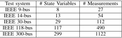
Table III shows the number of state variables and the number of measurements in the IEEE test systems. All these systems are assumed to be fully measured. Figures 15 and 16 show the matrix H of the IEEE 9-bus and 14-bus systems, respectively. The matrix H’s for the IEEE 30-bus, 118-bus, and 300-bus systems are space consuming; we do not include them here.
TABLE III
NUMBER OF STATE VARIABLES AND MEASUREMENTS IN THEIEEETEST
SYSTEMS
Test system # State Variables # Measurements
IEEE 9-bus 8 27
0
B B B B B B B B B B B B B B B B B B B B B B B B B B B B B B B B B B B B B B B B B B B B B B @
17.36 0.00 0.00 −17.36 0.00 0.00 0.00 0.00 0.00 0.00 16.00 0.00 0.00 0.00 0.00 0.00 −16.00 0.00 0.00 0.00 17.06 0.00 0.00 −17.06 0.00 0.00 0.00
−17.36 0.00 0.00 40.00 −10.87 0.00 0.00 0.00 −11.76 0.00 0.00 0.00 −10.87 16.75 −5.88 0.00 0.00 0.00 0.00 0.00 −17.06 0.00 −5.88 32.87 −9.92 0.00 0.00 0.00 0.00 0.00 0.00 0.00 −9.92 23.81 −13.89 0.00 0.00 −16.00 0.00 0.00 0.00 0.00 −13.89 36.10 −6.21 0.00 0.00 0.00 −11.76 0.00 0.00 0.00 −6.21 17.98 17.36 0.00 0.00 −17.36 0.00 0.00 0.00 0.00 0.00
0.00 0.00 0.00 10.87 −10.87 0.00 0.00 0.00 0.00 0.00 0.00 0.00 0.00 5.88 −5.88 0.00 0.00 0.00 0.00 0.00 17.06 0.00 0.00 −17.06 0.00 0.00 0.00 0.00 0.00 0.00 0.00 0.00 9.92 −9.92 0.00 0.00 0.00 0.00 0.00 0.00 0.00 0.00 13.89 −13.89 0.00 0.00 −16.00 0.00 0.00 0.00 0.00 0.00 16.00 0.00 0.00 0.00 0.00 0.00 0.00 0.00 0.00 6.21 −6.21 0.00 0.00 0.00 −11.76 0.00 0.00 0.00 0.00 11.76
−17.36 0.00 0.00 17.36 0.00 0.00 0.00 0.00 0.00 0.00 0.00 0.00 −10.87 10.87 0.00 0.00 0.00 0.00 0.00 0.00 0.00 0.00 −5.88 5.88 0.00 0.00 0.00 0.00 0.00 −17.06 0.00 0.00 17.06 0.00 0.00 0.00 0.00 0.00 0.00 0.00 0.00 −9.92 9.92 0.00 0.00 0.00 0.00 0.00 0.00 0.00 0.00 −13.89 13.89 0.00 0.00 16.00 0.00 0.00 0.00 0.00 0.00 −16.00 0.00 0.00 0.00 0.00 0.00 0.00 0.00 0.00 −6.21 6.21 0.00 0.00 0.00 11.76 0.00 0.00 0.00 0.00 −11.76
1
C C C C C C C C C C C C C C C C C C C C C C C C C C C C C C C C C C C C C C C C C C C C C C A
![Fig. 1.A power grid connecting power plants to customers via powertransmission and distribution networks (revised from [2])](https://thumb-us.123doks.com/thumbv2/123dok_us/1453193.1178032/1.612.341.533.220.387/power-connecting-plants-customers-powertransmission-distribution-networks-revised.webp)