Downloading Deep Web Data from Real Web Services

(1)

University of Windsor University of Windsor

Scholarship at UWindsor

Electronic Theses and Dissertations Theses, Dissertations, and Major Papers

2011

Downloading Deep Web Data from Real Web Services

Chong Fu

University of Windsor

Follow this and additional works at: https://scholar.uwindsor.ca/etd

Recommended Citation Recommended Citation

Fu, Chong, "Downloading Deep Web Data from Real Web Services" (2011). Electronic Theses and Dissertations. 322.

https://scholar.uwindsor.ca/etd/322

(2)

Downloading Deep Web Data from Real Web Services

by

Chong Fu

A Thesis

Submitted to the Faculty of Graduate Studies through Computer Science

in Partial Fulfillment of the Requirements for the Degree of Master of Science at the

University of Windsor

Windsor, Ontario, Canada

2011

(3)

Downloading Deep Web Data from Real Web Services

By Chong Fu

APPROVED BY:

______________________________________________ Dr. Kevin Li

Odette School of Business

______________________________________________ Dr. Jessica Chen

School of Computer Science

______________________________________________ Dr.Jianguo Lu, Advisor

______________________________________________ Dr. Alioune Ngom, Chair of Defense

(4)

DECLARATION OF ORIGINALITY

I hereby certify that I am the sole author of this thesis and that no part of this

thesis has been published or submitted for publication.

I certify that, to the best of my knowledge, my thesis does not infringe upon

anyone’s copyright nor violate any proprietary rights and that any ideas, techniques,

quotations, or any other material from the work of other people included in my thesis,

published or otherwise, are fully acknowledged in accordance with the standard

referencing practices. Furthermore, to the extent that I have included copyrighted

material that surpasses the bounds of fair dealing within the meaning of the Canada

Copyright Act, I certify that I have obtained a written permission from the copyright

owner(s) to include such material(s) in my thesis and have included copies of such

copyright clearances to my appendix.

I declare that this is a true copy of my thesis, including any final revisions, as

approved by my thesis committee and the Graduate Studies office, and that this thesis has

(5)

ABSTRACT

Data of deep web in general is stored in a database or a file system that is only

accessible via web query forms or through web service interfaces. One challenge of deep

web crawling is how to select meaningful queries to acquire data. There is substantial

research on the selection of queries, such as the approach based on the set covering

problem where greedy algorithm or its variation is used. These methods are not

extensively studied in the context of real web services, which may impose new

challenges for deep web crawling. This thesis studies several query selection methods on

Microsoft’s Bing web service, especially the impact of the ranking of the returns in real

data sources. Our results show that for unranked data sources, weighted method

performed a little better then un-weighted set covering algorithm. For ranked data

sources, document frequent estimation is necessary to harvest data more efficiently.

(6)

DEDICATION

This thesis is dedicated to my families who have supported me all the way since

the beginning of my studies with patience, understanding, and love.

Also, this thesis is dedicated to all those who helped me during my studies. If

each thing in my memory has weight, many things happened in the University of

(7)

ACKNOWLEDGEMENTS

I am heartily thankful to my supervisor, Dr. Jianguo Lu, who gave me critical

suggestions, honest criticisms and painstaking comments helping me to finish the

research and writing of this thesis. Without his guidance and support, this thesis would

not have been possible.

I also would like to thank my internal reader, Dr. Jessica Chen, my external

reader, Dr. Kevin Li, and my thesis committee chair, Dr. Alioune Ngom for spending

their time in reviewing this thesis and attending my thesis proposal and defence.

As well as, a special thanks to Frank Luo and Guanghui Luo with whom I built

the framework of WS-Crawler together in a course project.

Finally, I would like to show my gratitude to Yan Wang and Shaohua Wang for

(8)

TABLE OF CONTENTS

DECLARATION OF ORIGINALITY ... iii

ABSTRACT ... iv

DEDICATION ...v

ACKNOWLEDGEMENTS ... vi

LIST OF TABLES ... ix

LIST OF FIGURES ...x

I. INTRODUCTION 1 II. RELATED WORK 9 2.1 INCREMENTAL APPROACH ... 9

2.2 SAMPLING BASED APPROACH ... 13

III. SET COVERING PROBLEM 16 IV. SET COVERING ALGORITHMS 21 4.1. GREEDY ALGORITHM ... 21

4.2. WEIGHTED ALGORITHM ... 26

4.3. RANKING PROBLEM ... 31

V. EXPERIMENTS 35 5.1. EXPERIMENTAL ENVIRONMENT ... 35

5.2. EVALUATION CRITERIA ... 39

5.3. EXPERIMENTS ... 41

5.3.1 Sample Databases Creation ...41

5.3.2 Ranking Strength Observation on the Data Sources ...42

5.3.3 Comparison on Query Selection Policies ...43

(9)

VI. CONCLUSION AND FUTURE WORK 52

6.1 CONCLUSION ... 52

6.2 FUTURE WORK ... 53

APPENDIX I 55

REFERENCES 60

(10)

LIST OF TABLES

TABLE 1:GREEDY ALGORITHM EXAMPLE (1) ... 23

TABLE 5:WIGHTED GREEDY ALGORITHM EXAMPLE (1) ... 29

TABLE 8:DESCRIPTION OF DATA SOURCES AND SAMPLE DATABASES ... 41

TABLE 9:PERCENTAGE OF TERMS WITHIN K ... 42

TABLE 10:EXPERIMENT RECORD CHART ... 43

TABLE 11:COMPARISON OF DF-WEIGHTED AND OTHERS ... 48

TABLE 12:COMPARISON OF GREEDY AND WEIGHTED ... 49

(11)

LIST OF FIGURES

FIGURE 1:A PART OF ARXIV.COM HOME PAGE ... 1

FIGURE 2:ACCESSING BING CONTENT BY TWO WAYS: SEARCH INTERFACE OR WEB SERVICE ... 3

FIGURE 3:HTML SEARCH FORM OF AMAZON BOOK STORE ... 5

FIGURE 4:VIRTUAL INTEGRATION –COMPARISON SHOPPING ... 6

FIGURE 5:STATISTIC TABLE:DOCUMENT FREQUENCY OF TERMS ... 11

FIGURE 6:THE FRAMEWORK OF LU’S SAMPLE-BASED APPROACH ... 15

FIGURE 7:FORMALIZATION OF THE QUERY SELECTION PROBLEM ... 17

FIGURE 8: SET-COVERING FORMALIZATION (EXAMPLE) ... 23

FIGURE 9: THE WHOLE PROCEDURE OF GREEDY ALGORITHM ... 25

FIGURE 10: THE WHOLE PROCEDURE IN SET COVERING VIEW (BY WEIGHTED GREEDY ALGORITHM) ... 30

FIGURE 11:A DEEP WEB SITE USUALLY SET UP A RETURN LIMITATION ... 32

FIGURE 12:THE RESULTS FOR “SITE:CS.BERKELEY.EDU VAZIRANI” ... 35

FIGURE 13:RESPONSE PAGE FROM BING WEB SERVICE ... 36

FIGURE 14:THE USER INTERFACE OF OUR CRAWLER ... 38

FIGURE 15:DATAFLOW DIAGRAM OF OUR CRAWLER ... 39

FIGURE 16:PERFORMANCE DIAGRAMS OF CS.BERKELEY.EDU ... 45

FIGURE 17:PERFORMANCE DIAGRAMS OF UWATERLOO.CA ... 46

FIGURE 18:PERFORMANCE DIAGRAMS OF CTV.CA ... 47

(12)

CHAPTER I

INTRODUCTION

The Deep Web [4] data refer to the content that is dynamically generated from

databases or file systems. The information served on the Deep Web is accessible through

query interfaces such as html forms or web services. Many organizations, such as

“Arxiv.org”, “Bing.com” or “Amazon.com”, provide web service interfaces to access

their deep web data. Since data are hidden behind query interfaces, the deep web are also

called as the Hidden Web [7] [10] or invisible web [10]. The figure below is a part of the

home page of “Arxiv.org”. This website provides a large number of academic documents.

In most cases, users look for the document that they want by using the html query form at

the top.

Figure 1: A part of Arxiv.org home page

The deep web often contains a large amount of documents which are often of high

quality and value to users. Since there are no static links to those deep web documents,

deep web content is beyond the reach of traditional search engines [5]. In order to access

(13)

the query. According to the research [4], the content of deep web is about 500 times

greater than that visible to conventional search engines. Hence how to utilize the deep

web content becomes a major challenge within the information retrieval community.

The thesis focuses on the task of downloading the deep web data from real web

services. We have developed a web-service crawler named “WS Crawler”, implemented

and experimented with four query selection algorithms for deep web crawling. Our

objective is to evaluate their efficiency for retrieving data from different real data sources

via web service.

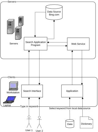
In order to share their data to users, some deep web sites provide web service for

client application to access their online databases. Web service is a technology that

enables application-to-application interaction over the network – regardless of platform,

language, or data formats. By exposing web APIs (Application Programming Interfaces)

on the network, functionalities of web service can be activated using HTTP requests.

Through these APIs, client application can access remote content. Advantages of using

web services include: no need to fill html query form and no need to extract relevant data

(14)

User 1 _{User 2} Servers

Servers

Data Source Bing.com

Search Application

Program Web Service

Clients

Search Interface Application

Laptop Workstation

Type in keyword

Data Dictionary Select keyword from local data source

(15)

Deep web content in general is stored in a database. By the type of the database,

they can be categorized either as an unstructured (textual) database or as a structured

database [24]. An unstructured database is a site that mainly contains plain-text

documents (e.g., legal documents). In contrast, a structured database is a site that often

contains relational data, such as an online book store that may have multiple fields such

as title, author, and ISBN etc. For a textual database, the search interface usually provides

a simple keyword textbox. Conversely, the interface to a structured database may allow

the users to submit multiple attributes (e.g., searching cars by company name, brand, or

the year of production). The interface may contain a combination of text box, radio

button, dropdown menu etc.

Textual database mainly contains plain-text documents, such as papers, law

documents, and news articles etc. Html query form of a textual database usually only

provides a single textbox to fill in keywords, as shown in Figure 1. It is an html search

form from arXiv.org. The arXiv database is textual. It contains about 500,000 papers.

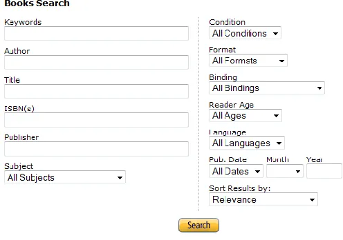
Structured database mainly contains relational data, such as on line store database. Html

(16)

Figure 3: Html Search Form of Amazon Book Store

Here is an example from Amazon on line book store. You can search a book by

author, title, or ISBN etc. Our research is related to textual database.

With millions of databases connected to the internet, we cannot ignore data

hidden behind search interface. To utilize deep web content, virtual integration and

surfacing are the two main applications.

The virtual integration approach [9] [25] is to provide a uniform interface to

access a specific kind of data from different deep web sources. To build such an

application, we need to identify the domain (e.g., book, airline ticket, or real-estate) of

each deep web and analyze the html search interface. Thus, an automatic integration

system often contains an automatic identification system and a semantic system. The

identification system is to analyze the query interface or contents of a deep web site and

to identify the domain that it belongs to. For example, we have known a large amount of

deep web sites. Now, we are only interested in the online book store sites. So a first step,

(17)

After that, we already have a set of deep web sites in a domain of interest. Then, we need

to build a unified query interface to search those sites at the same time. To create a

unified query interface, a semantic system is necessary to build and manage semantic

mappings on the search interfaces of those deep web sites. In short, it is to map queries to

difference search interfaces. Then integration system will extract, combine, and rank the

results retrieved form difference data sources. Finally, present regenerative results to the

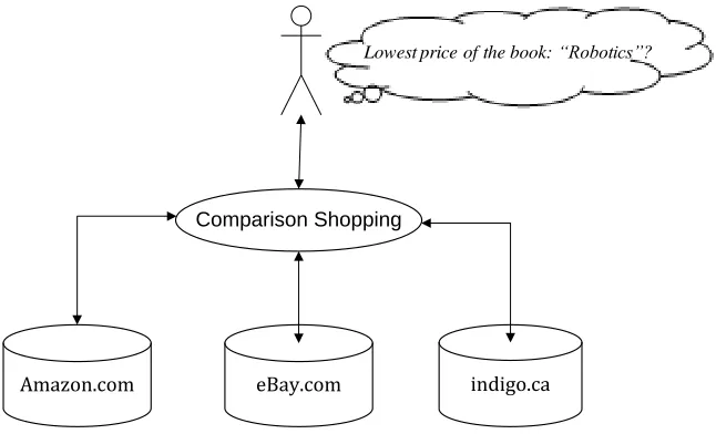
users. Generally, a virtual integration provides more experience to user besides search.

For instance, we search a book in a virtual integration search engine. The results are

retrieved from the difference online book stores, such as “amazon.com”, “ebay.com”, and

“indigo.ca”. In addition to return those results, the search engine also provides the best

price of the book. For that reason, virtual integration is more suitable for the structure

databases.

Comparison Shopping

Amazon.com eBay.com indigo.ca

Lowest price of the book: “Robotics”?

Figure 4: Virtual Integration – Comparison Shopping

The surfacing approach is also called deep web crawling which downloads hidden

(18)

search engine index today. In general, the challenges of deep web crawling include: how

to process html query form [18]; how to extract relevant data from result pages [15] [2];

and how to choose a set of queries [20] [16] [18] [21] [3] [22]. An excellent crawler

should surface the deep web sites automatically. Hence, the crawler needs an approach to

process html query form and extract relevant data from result pages automatically. We

use web service in our experiments, so we do not need to process the html query form,

and the results is XML file format. For that reason, we can focus on query selection

problem.

The real environment usually sets up a return limitation for the maximal number

of results. Most of the earlier methods are designed to download a deep web site without

return limitation. Therefore, they cannot work well when return limitation exists. We

present a DF-Weighted Greedy algorithm to cope with this challenge.

Experiments are carried on three data sources which are “cs.berkeley.edu”,

“uwaterloo.ca”, and “ctv.ca”. The size of the first data source is small, which contains

about 30,000 web pages. This means return limitation problem is not serious in this data

source, because the number of most matches will not surpass the limit. The other two

data sources are larger than the first one. The number of web pages of “uwaterloo.ca” and

“ctv.ca” are approximate 150,000, and 140,000. The experimental results show our

DF-Weighted greedy works well when downloading the data from the last two data sources.

In addition to the introduction section, there are five sections in this thesis.

Section 2 introduces relative work. It includes the difference types of query selection

approaches for deep web crawling. Section 3 introduces set covering problem and how

(19)

three sampling based algorithms: Greedy, Weighted Greedy and DF-Weighted Greedy.

Section 5 describes our experiments and gives the results. Finally, the conclusion and

(20)

CHAPTER II

RELATED WORK

The key problem of deep web crawling is how to choose a set of queries to submit

to the query form. There are many ways to select keywords.

A primitive solution can be randomly selecting some words from a dictionary.

However this solution is not efficient, due to that a large number of rare queries may not

match any page, or there could be many overlapping returns. Instead of selecting

keywords from dictionary, several algorithms have been developed to select keywords.

Currently, most approaches that had been developed are to analyze and choose the

queries from the documents downloaded from the previous queries submitted to the deep

web database. They can be categorized as: Graph approach [1] [24], Incremental

approach [20] [18], and Sampling based approach [16] [3] [22]. Graph approach is used

to download structured database, so it is not discussed in my thesis.

2.1 Incremental approach

Incremental approach selects queries from the documents that have been

downloaded. The number of documents increases as more queries are sent, thus this kind

of approach are called incremental approach.

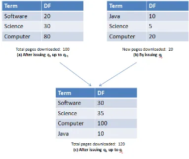
Ntoulas et al. [20] propose an adaptive method. Their approach selects the query

returning most new documents per unit iteratively. Since there is no prior knowledge of

(21)

document frequencies based on the documents already downloaded. From this estimation

and the occurrences of the queries in the downloaded documents, the number of matched

new documents can be estimated. They propose two ways to estimate. The first method

which is called independence estimator assumes that the occurrence probability of a term

in the subset of documents is equal to that in the entire document set. Based on the

frequency of a term in the subset of documents N(qi | subset collection), the method can

estimate how many times a particular term occurs in the entire document set N(qi). Then

we can estimate the number of new documents by: Nnew(qi) = N(qi) - N(qi | subset

collection).

The method of Zipf estimator [13] is to estimate the frequency of terms inside

document collection by following a power law distribution. That is, the frequency of a

term within the document collection is given by the formula:

N(qi)= α (r +β )-Ƴ, (1)

where r is the rank of the term and α , β , and Ƴ are constants that depend on the

document collection. Based on the subset of documents that we have downloaded, we can

estimate α , β , and Ƴ by the approach which is mentioned in [20]. Given the ranking r

of a term inside the subset of document collection, N(qi) can be calculated by formula

(1). They compare three keyword selection policies: random (Keywords are randomly

selected from dictionary.), generic-frequency (Keywords are selected from

5.5-million-web-page corpus based on their decreasing frequency.), and their adaptive algorithm. The

experimental result shows that adaptive algorithm (Keywords are selected from the

(22)

[20], select queries from an incremental document collection. Therefore, we call this kind

of approach as incremental approach. Incremental approach selects queries from an

incremental document collection. That means you need to analyze each document once it

is downloaded and calculate the document frequency again for each term. This step will

be very time-consuming, if we count the document frequency for every query at each

round. In order to calculate document frequency efficiently, Ntoulas’ solution computes

the document frequency by updating the query statistics table after we submit a new

query and download more documents. However maintaining this table still is difficult.

(23)

The sampling-based approach [16] [3] firstly creates a sample database and builds

a set of queries from the sample database, rather than iteratively selecting keywords from

an incremental subset of document collection until crawling ends.

Madhavan et al. [18] develop a deep-web crawling system. Because the system is

an industry product, it needs to consider how to select seed queries. Their system detects

the feature of the query interfaces. Since they need to process difference languages, their

approach does not select queries from a dictionary. Instead, they select the seed queries

from the html query form. After that, the iterative probing and keyword selection

approach is similar to that proposed in [20].

Their query selection policy is based on TF-IDF that is the popular measure in the

information retrieval. TF-IDF measures the importance of the word by the formula

below.

(2)

This formula consists of two parts: tf(w, p) is the term

frequency of the term w in page p, and measures the importance of the word w in page

p.

,

where nw,p represents the number of times a word w occurs in web page p;

is the total number of terms in page p.

idf (w) (inverse document frequency) measures the importance of the word

among all web pages, and is calculated by

(24)

Madhavan et al’s method adds the top 25 words on every web page sorted by their

TF-IDF values into the query pool. From the query pool, they remove the following two

kinds of terms.

 Eliminate the high frequency terms, such as the terms that have appeared in

many web pages (e.g. over 80% ), since these terms could be from menus or

advertisements.

 Delete the terms which occur only on one page, since many of these terms

are meaningless words that are not from the contents of web pages, such as

nonsensical or idiosyncratic words that could not be indexed by the search

engine.

The remaining words are issued to deep web as queries and a new set of web

pages are downloaded. Then this is repeated again in the new iteration. Additionally, their

approach emphasizes breadth oriented crawling that is quite different to prior researches.

They observed the statistic data on Google.com and found the results returned to users

were more dependent on the number of deep web sites. They analyzed 10 millions of

deep web sites. They discovered the top 10,000 deep web sites accounted for 50% of

Deep-Web results, while even the top 100,000 deep web sites only accounted for 85%.

This observation causes their focus on crawling as many deep web sites as possible,

rather than surfacing on specific deep web sites.

2.2 Sampling based approach

In [21] [3], Barbosa et al. propose an approach to siphon the deep web by

(25)

algorithm selects the highest frequency keyword from the potential keyword list and is

expected to lead a high coverage. It is composed of two phases: phase 1 selects a set of

words from the html search form and randomly issues them until a non-empty result page

is returned. By extracting high-frequency words from the results page, their algorithm

creates an initial keyword list. Then it iteratively updates the frequency of words in the

list and adds new high-frequency words into the list by randomly issuing the word in the

list until the number of submission reaches the threshold. In phase 2, the approach selects

the most frequency keyword from the keyword list to construct a new query in each

round until the number of submission is up to maximum times.

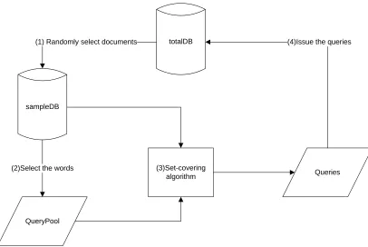
In [16], Lu et al. further improve the sampling based method. Keywords are

selected from a fixed sample database by a set covering algorithm. Those queries which

can cover most documents in the sample database are expected to cover most of data in

the entire database. The framework of this approach is showing in the figure below. For

sampling based approach, queries are selected from the sample set of documents from the

total database. This approach consists of three phases:

1) Create a sample DB: Issue the initial keywords to the total DB, obtain the

matched documents, and then construct a sample database;

2) Construct the query pool: Analyze all the documents in the sample DB, apply

set-covering algorithm to select the keywords and generate a query pool;

3) Send the queries to Total DB to retrieve documents.

The advantage of this method is that only a small part of documents need to be

(26)

documents. Our focus is sampling based approach. Hence, more detail about sampling

based approach will be described in Chapter IV.

totalDB

sampleDB

QueryPool

(1) Randomly select documents

(2)Select the words (3)Set-covering

algorithm Queries (4)Issue the queries

(27)

CHAPTER III

SET COVERING PROBLEM

One of key problems of deep web crawling is to select a set of meaningful

keywords. Selecting queries from a document collection is a popular method. Ntoulas et

al [20] are the first to use set-covering problem to represent the query selection problem.

Set-covering problem is a typical NP problem [6]. It can be described as the

following: given a finite set U and a family X of subsets of U, the solution is to find a

cover C whose union is U and it is a subfamily of X. The set-covering problem can be

divided into two problems. One is the set covering decision problem, i.e., given a pair

(U,X) and an integer k; the question is to decide whether there is a cover of size k or less.

The set-covering decision problem is NP-Complete. The other is the set covering

optimization problem, i.e., given a pair (U,X) the goal is to find minimum-size subsets

O whose elements cover all of U. The set covering optimization problem is NP-hard [11].

More formally, given U and X as follows:

(28)

, and the cost of O is minimum.

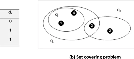
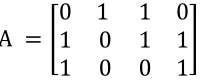
The input of the set covering problem is often represented by a query-document

matrix as illustrated in Figure 7. In Figure 7 (a), the matrix represents the relationship

between three queries (q1, q2, q3) and four documents (d1, d2, d3, d4). If the cell (i,j) is

1, query in the ith row (qi) is contained in the document in the jth column (dj). This

matrix representation can be illustrated by Figure 7 (b). The rectangle in Figure 7 (b)

represents the whole document set. Each document is represented as a black point inside

the rectangle. Every oval in the figure (b) represents a set of documents covered by a

query.

Figure 7: Formalization of the query selection problem

The minimum set cover problem can be formulated as the Integer Linear

Program [11]. According to the integer linear program formulation in [11], we formalize

the set covering problem for query selection as the following: Let A is an m*n matrix of

0 and 1 representing a document collection like Figure 7(a). The set covering problem is

to find a solution m-vector S whose Si = 0 or 1 ( i = 1,…,m ) that is representing whether

the query i is either chosen or not. Ci is an m-vector of positive integer that is

(29)

of ones that is representing every document in the matrix A is covered. More formally, it

can be formulated as below:

(3)

(4)

where Si = {0,1| i = 1,…,m}; Ei = {1|i=1,…,n}; Ci = { i = 1,…,m}.

For instance, there are two solutions: {q1, q2} and {q1, q3} for the problem in the

Figure 7. From the Figure 7 (a), we can know:

There are three subset q1, q2, and q3 in the matrix A. By the definition of C:

First step, we verify both solutions are satisfied with the condition.

Subject to:

(30)

Thus,

LHS=

For the solution {q1, q3}:

Thus,

LHS=

Therefore, both solutions subject to the condition:

In the next step, we calculate the cost for both solutions.

For the solution {q1, q2}:

Total cost =

(31)

Total cost =

By the objective function Formula (3), we know the solution 2 is better than the

(32)

CHAPTER IV

SET COVERING ALGORITHMS

Set covering problem has been proved to be NP-Complete [6]. Optimal solution is

hard to obtain within polynomial time. Various optimization algorithms are developed,

such as Greedy, Weighted Greedy, Genetic, and Clustering etc. Traditional Greedy and

Weighted Greedy algorithms will be implemented in experiment section.

4.1. Greedy Algorithm

One popular algorithm for set covering problem is the greedy algorithm which

chooses queries according to one rule: at each round, always selects the query that covers

the largest number of new documents per unit cost. A greedy algorithm makes the locally

“best” choice at each stage, but it is not the best choice globally. Assuming we have

constructed a query pool with a set of queries, greedy algorithm is to find the most

effective query from the query pool.

Greedy Algorithm:

Input: m * n Matrix A;

Output: A solution m-vector S;

(33)

B = A;

E is an n-vector, and initializes every element to 1;

S and c is an m-vector, and initialize every element to 0;

while {

for( i=1; i<= m; i++){

newi = ;

ci = dfi / newi;

}

Find a k which minimizes ck ;

Sk =1;

Remove the kth row and jth column from B, if cellij =1;

}

for (j = 1; j <=m; j++){

if(Sj = 1 and Aj is redundant) Sj = 0;

}

(34)

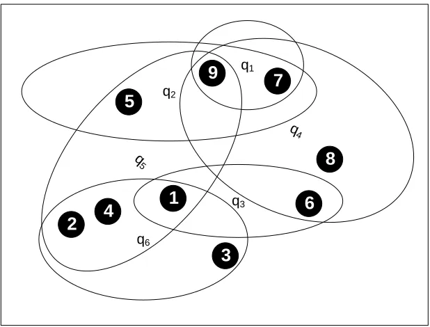
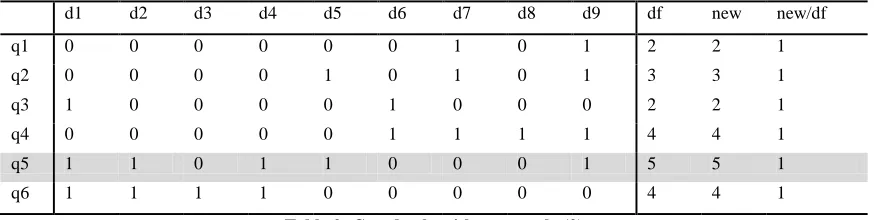
For example, the matrix below represents a sample database which contains nine

documents (d1, d2, d3, …, d9). Suppose our query pool includes six queries (q1, q2, q3,

q4, q5, and q6).

d1 d2 d3 d4 d5 d6 d7 d8 d9

q1 0 0 0 0 0 0 1 0 1

q2 0 0 0 0 1 0 1 0 1

q3 1 0 0 0 0 1 0 0 0

q4 0 0 0 0 0 1 1 1 0

q5 1 1 0 1 1 0 0 0 1

q6 1 1 1 1 0 0 0 0 0

Table 1: Greedy algorithm example (1)

By the rule mentioned above, we can convert the matrix to a set-covering problem

as the figure below. We choose sets (queries) by greedy algorithm to cover all

documents. The whole procedure is listed as following:

1 2 3 4 q6 q2 q1 5 6 7 8 9 q3 q₄ q 5

(35)

Round 1: Add q5 into query pool, the value of new/df for each query is equal to 1.

As a result, we randomly select the query with largest df.

d1 d2 d3 d4 d5 d6 d7 d8 d9 df new new/df

q1 0 0 0 0 0 0 1 0 1 2 2 1

q2 0 0 0 0 1 0 1 0 1 3 3 1

q3 1 0 0 0 0 1 0 0 0 2 2 1

q4 0 0 0 0 0 1 1 1 1 4 4 1

q5 1 1 0 1 1 0 0 0 1 5 5 1

q6 1 1 1 1 0 0 0 0 0 4 4 1

Round 2: Add q4 into query pool, since new/df(q4) = ¾ is maximum value in the

last column.

q1 0 0 0 0 0 0 1 0 1 2 1 1/2

q2 0 0 0 0 1 0 1 0 1 3 1 1/3

q3 1 0 0 0 0 1 0 0 0 2 1 1/2

q4 0 0 0 0 0 1 1 1 1 4 3 3/4

q5 1 1 0 1 1 0 0 0 1 5 -- --

q6 1 1 1 1 0 0 0 0 0 4 1 1/4

Round 3: Add q6 into query pool, since new/df(q6) = ¼ is maximum value in the

last column.

q1 0 0 0 0 0 0 1 0 1 2 0 0

q2 0 0 0 0 1 0 1 0 1 3 0 0

q3 1 0 0 0 0 1 0 0 0 2 0 0

q4 0 0 0 0 0 1 1 1 1 4 -- --

q5 1 1 0 1 1 0 0 0 1 5 -- --

q6 1 1 1 1 0 0 0 0 0 4 1 1/4

Therefore, the Solution of this example is {q5, q4, q6}.

(36)

1 2 3 4 q6 5 6 7 8 9 q₄ q 5 1 2 3 4 5 6 7 8 9 q₄ q 5 1 2 3 4 5 6 7 8 9 q 5

Figure 9: the whole procedure of Greedy Algorithm

Check whether the solution {q5, q4, q6} covers all the documents by:

Thus, =

(37)

Next, calculate the cost of the solution {q5, q4, q6}:

Total cost =

4.2. Weighted Algorithm

Traditional set covering algorithms do not work well when applied to deep web

crawling due to various special features of the application domain. Typically, most set

covering algorithms ignore the distribution of document frequencies. In [34], the authors

developed a new set covering algorithm that targets the deep web crawling. Instead of

straightforward greedy set covering algorithm, it introduces weights into the greedy

strategy. They use Document Frequency df (the number of documents that contain a

specific earlier query.), Document Weight dw (the inverse of the number of terms in QP

that occurs in the document), and Query Weight qw(the sum of the document weights of

all documents containing term q). The weighted greedy algorithm is based on choosing

the query with the smallest df/qw.

To improve simple greedy algorithm and decrease the overlap, the weighted

(38)

greedy algorithm instead of a straightforward greedy set covering algorithm. The

definitions are introduced as follows:

Definition 3 (Document Weight): Let D={d1,…,dm} be the SampleDB and

QP={q1,…,qn} be the QueryPool. We consider each document as a set of terms and use

the notation qj di to indicate that a term qj occurs in the document di. The weight of a

document with respect to QP and di (1≤i≤m), denoted by dw(di, QP) (or dw for shot), is

the inverse of the number of terms in QP that occurs in the document di, i.e.

Definition 4 (Query Weight): The weight of a query qj (1≤j≤n) in QP with

respect to D, denoted by qw(qj, QP) (or qw for short), is the sum of the document weights

of all documents containing term qj, i.e.,

Weighted Greedy Algorithm:

Input: m * n Matrix A;

Output: A solution m-vector S;

(39)

B = A;

E is an n-vector, and initializes every element to 1;

S and c is an m-vector, and initialize every element to 0;

While {

for( i=1; i<= m; i++){

;

ci = dfi / qwi;

}

Find a k which minimizes ck ;

Sk =1;

Remove the kth row and jth column from B, if cellij =1;

}

for (j = 1; j <=m; j++){

if(Sj = 1 and Aj is redundant) Sj = 0;

}

return S;

The weighted greedy algorithm always selects the next query with the largest

“qw/df". Based on this rule, the weighted greedy algorithm selects keywords from

(40)

much better result than the simple greedy method in the SampleDB, so it should be

expected to retrieve a better result in the TotalDB.

By Weighted Greedy Algorithm, we can get the Solution #2(q6, q4, q2) for

example 2.

Round 1:

d1 d2 d3 d4 d5 d6 d7 d8 d9 df qw qw/df

q1 0 0 0 0 0 0 0.333 0 0.25 2 0.583 0.292

q2 0 0 0 0 0.5 0 0.333 0 0.25 3 1.083 0.361

q3 1 0 0 0 0 0.5 0 0 0 2 1.5 0.75

q4 0 0 0 0 0 0.5 0.333 1 0.25 4 2.083 0.521

q5 0.5 0.5 0 0.5 0.5 0 0 0 0.25 5 2.25 0.45

q6 0.5 0.5 1 0.5 0 0 0 0 0 4 2.5 0.625

Table 5: Wighted Greedy algorithm example (1)

Round 2:

q1 0 0 0 0 0 0 0.333 0 0.25 2 0.583 0.292

q2 0 0 0 0 0.5 0 0.333 0 0.25 3 1.083 0.361

q3 1 0 0 0 0 0.5 0 0 0 2 0.5 0.25

q4 0 0 0 0 0 0.5 0.333 1 0.25 4 2.083 0.521

q5 0.5 0.5 0 0.5 0.5 0 0 0 0.25 5 0.75 0.15

q6 0.5 0.5 1 0.5 0 0 0 0 0 4 - -

Table 6: Wighted Greedy algorithm example (2)

Round 3:

q1 0 0 0 0 0 0 0.333 0 0.25 2 0 0

q2 0 0 0 0 0.5 0 0.333 0 0.25 3 0.5 0.1667

q3 1 0 0 0 0 0.5 0 0 0 2 0 0

q4 0 0 0 0 0 0.5 0.333 1 0.25 4 - -

q5 0.5 0.5 0 0.5 0.5 0 0 0 0.25 5 0.5 0.1

q6 0.5 0.5 1 0.5 0 0 0 0 0 4 - -

(41)

We transfer the whole procedure of choosing sets by the weighted greedy

algorithm in set covering view as picture below.

1 2 3 4 q6 q2 5 6 7 8 9 q₄ 1 2 3 4 q6 5 6 7 8 9 q₄ 1 2 3 4 q6 5 6 7 8 9

Figure 10 : the whole procedure in set covering view (by Weighted Greedy Algorithm)

Check whether the solution {q6, q4, q2} covers all the documents by:

(42)

=

Therefore, all the documents are covered by the solution {q6, q4, q2}.

Next, calculate the cost of the solution {q6, q4, q2}:

Total cost =

By comparing with the cost in the example of section 4.1, we can see the solution

given by weighted greedy algorithm is better than the solution generated by conventional

greedy algorithm.

4.3. Ranking Problem

Return limitation and ranking policy results in the ranking problem. Many hidden

(43)

of documents, the deep web sites only return at most k documents. This is called return

limitation. Ranking policy is the rule of sorting results.

Figure 11: A deep web site usually set up a return limitation

Ranking policy generally could be either static or dynamic. A static ranking, say

the web service of “twitter.com”, sorts the results by the order of date and time. A

dynamic ranking could sort the results by the relevance to the query. Those documents

that are highly related to the search query will be listed on the top. The more relevant to

the search query, the position of a document is closer to the top. However for the

commercial search engines, the ranking policy is much more complex. Generally, the

commercial search engines rank the results mainly by the order of relevance and

importance. The relevance of web pages will be evaluated by many factors: such as the

number of occurrence times, the position of appearance, and whether the title contains the

term etc. The importance of web pages will be measured by other criteria, e.g., the

number of links to the web page from the other websites and the reputation of those

websites. Once the search engine has sorted a list of documents with their scores, it will

choose the top k documents as the results for a query.

The return limitation gives us a great challenge to download data from the deep

(44)

select the terms with high document frequency as queries. These queries are supposed to

match a large number of documents. However because of the return limitation, only at

maximal k number of documents can be downloaded.

When a deep web site sets up a return limitation, the rule of ranking is also a

critical problem for deep web crawling. By Lu et al. [17]’s previous research, if a search

engine commits static ranking rule, there is the following result:

(5)

where M is the number of documents that can be downloaded; k is the return

limitation; dfq is the lower bound of document frequencies of all queries sent; N is data

source size.

This formula shows that if we select high frequency terms as queries, fewer

documents can be downloaded. For example, suppose we keep submitting queries whose

document frequency is greater than 200 to a deep web search engine whose k equals to

100. By Equation 5, if the search engine lists the result with static ranking policy, the

total number of documents which can be downloaded should be:

No matter how many queries are sent. Despite dynamic ranking policy could

alleviate such a ranking problem, those popular terms are still not a good choice.

Therefore our idea is to select the queries whose document frequencies are less than k.

(45)

whose document frequency is less than k. However we do not know the document

frequency of a term until we submit the term as query. Hence, we have to estimate the

document frequency of a term. One straight-forward method is to estimate the document

frequency of a term in the total database by using sample database. Assuming that the

probability of a term in the sample database and the total database is the same, the

document frequency of a term can be estimated by:

(6)

The method that we apply document frequency estimation method on the

weighted greedy algorithm to choose queries from the sample database is called

DF-Weighted algorithm.

DF-Weighted firstly estimates the document frequency of total database for all the

terms in the sample database. The terms whose document frequency is less than k are

selected to generate a matrix with all the documents covered by them. After that, the

matrix is processed as the input of weighted greedy algorithm. Then weighted greedy

(46)

CHAPTER V

EXPERIMENTS

5.1. Experimental Environment

The task of our experiments is to evaluate various downloading policies described

in Charter 3 on real deep web sites. We select Bing web service as our test bed and use

slices of the data indexed in Bing as various deep web data sources. Those slices can be

web sites, such as cs.berkeley.edu, which can be accessed using Bing search syntax “site:

cs.berkeley.edu”. Such search interface and the results from Bing are quite similar to the

search box provided by the web site itself. Thus we can simulate the access to almost all

the web sites as searchable deep web data sources.

For example, if we plan to test on “cs.berkeley.ca”, we can repeatedly submit

queries to Bing search engine like “site: cs.berkeley.edu [query]”, as shown in Figure 12.

(47)

In this thesis, instead of using html form search interface, we submit the queries to

Bing web service. Therefore we do not need to fill the html query form and extract the

data from html result pages.

Bing API provides HTTP Get to implement the process of submitting requests. A

request to the HTTP endpoint consists of an HTTP GET request to the appropriate URI.

There are two URIs, one for XML results and one for JSON results. The XML format is

used in our experiment. So we submit our requests to the URI: “

http://api.search.live.net/xml.aspx” . If we want to query the site “cs.berkeley.edu” for

the pages matching the term “large”, the complete request sent to Bing web service is:

http://api.search.live.net/xml.aspx?Appid=<AppID>&query=site:cs.berkeley.edu%20larg

e&sources=web.

Figure 13: Response page from Bing web service

The picture above is a portion of response page. Several returned elements are

explained below:

1) The Total element, “<web:Total>”, contains the estimated number of results

(48)

inaccurate number, we use our own estimation of the size by exhaustively

sending a very large number of queries.

2) The Offset element, “<web:offset>”, indicates the current position of the

result set you are processing. You can change Offset using the optional

Offset parameter. Each response page at most contains 50 results. This

means, if a query matches 100 results, you need to submit this query twice to

Bing web services. For example, if you wanted to ask for 50 results at a time,

you would pass “web.count=50” as part of the query string. If you wanted to

get the next 50 results after getting the first results, you would pass

“web.offset=51”. The full URI would be as the following:

http://api.search.live.net/xml.aspx?

Appid=<AppID>&query=site:cs.berkeley.edu%20large&sources=web

&web.count=50&web.offset=51

Bing web service imposes some challenges for deep web crawling, such as return

limitation, ranking of the returns, paginated results, and inter-page overlapping.

1) Return limit, only top one thousand of results can be returned per query.

2) Inter-page overlap: Bing web service sometimes even could return same

documents when you issue a query. In our experimental result, we had pruned this

kind of duplicate.

3) Ranking criteria: Comparing local simulation data source, we do not know the

rule of Bing search engine for ranking results. This problem also gives us a new

(49)

In order to facilitate the experiment on Bing web service, we build a web service

crawler. The figure below is the GUI and the dataflow diagram of our crawler. To make

the crawler more flexible, the system is independent of algorithms. A query selection

algorithm output the queries to a text file. And our WS-Crawler read the queries from the

text file and creates a query pool.

(50)

Figure 15: Dataflow diagram of our crawler

5.2. Evaluation Criteria

When we select queries from documents by different algorithms, the solutions

should be also different. In order to evaluate which solution performance is better, we

select Hit Rate [22] and Overlapping Rate [22] as our evaluation criteria.

Hit rate is to measure how many percentages of documents are harvested by the

crawler. So Hit Rate is equal to the number of unique documents downloaded divide by

the total number of documents in the web database.

(51)

Overlapping rate is used to measure the communication cost. In the formula (8),

Overlapping Rate is equal to the number of documents downloaded, including duplicate

documents divide by the number of unique documents downloaded.

(8)

For example, we have a document set which contains 4 documents (d1, d2, d3, and

d4). There are 3 queries (q1, q2, and q3) in our query pool. The relation between the

documents and queries is shown in the Figure 7. We have two solutions that can cover all

of documents. One is {q1, q2}, and the other is {q1, q3}.

Solution 1:

Solution 2:

The hit rate for both solutions is same. However the overlapping rate of solution 2

is lower, this means the solution 2 reaches 100 percent coverage with less documents

(52)

5.3. Experiments

5.3.1 Sample Databases Creation

The experiments are carried on three data sources: “cs.berkeley.edu”,

“uwaterloo.ca”, and “ctv.ca”. For each data source, we create three samples whose sizes

are approximately 5%, 10%, and 20% of the original data source. We create three

different sample databases for each data source. The sizes of those sample databases are

approximately 5%, 10%, and 20%. the sample databases are built as follows:

1) Randomly select queries from the Webster dictionary that contains about

59000 terms;

2) Issue some of those queries to Bing web service and download more than 20%

documents;

3) All those documents can be divided into many portions by queries. We

randomly compose those sets of documents into about 5%, 10%, or 20%

document collection;

4) Use Lucene (a tool to index the documents) to create sample databases.

Table 8: Description of Data Sources and Sample Databases

Data Source cs.berkeley.edu uwaterloo.ca ctv.ca

Approximate

(N)

30,000 150,000 140,000

Sample Size

1548 8019 6911

3319 13924 14504

(53)

5.3.2 Ranking Strength Observation on the Data Sources

Ranking problem has a great effect on the performance of downloading data from

the deep web sites. Thus to measure the ranking strength of the data sources is necessary.

Ranking strength is measured by calculating the percentage of queries which are within

the return limitation. All the selected terms whose document frequency is bigger than 1

from the three sample databases (20%N). All those terms are submitted to the Bing web

service and k has default value 1000. Then we can get the number of terms whose

document frequencies are less than 100 and 200.

Table 9: Percentage of Terms within k

From Table 9, we can make the following observation:

Because the size of data source “cs.berkeley.edu” is small, the matches of the

most of queries do not exceed the return limit. Therefore ranking strength in this data

source is weak.

Despite the size of “ctv.ca” and “uwaterloo.ca” is very close, words of “ctv.ca”

are very generic. The percentage of popular terms of “ctv.ca” is higher than

“uwaterloo.ca”. Hence ranking strength of “ctv.ca” is stronger than “uwaterloo.ca”.

Data Source

Approximate

(N)

Terms

Num (tn)

df100 df100 /tn df200 df200 / tn

Ranking

Strength

cs.berkeley.edu 30,000 48,522 36,546 75% 39,627 81% weak

uwaterloo.ca 150,000 271,530 173,438 64% 184,403 68% middle

(54)

5.3.3 Comparison on Query Selection Policies

We evaluate four query selection policies on 27 combinations of experiment

environments. For each data source, we set up three different return limitations (100, 200

and 1000) and three different sample databases (approximately 5%, 10%, and 20%). We

evaluated the four query selection policies as the following:

 Random: Randomly selects queries from the Webster dictionary;

 Sampling based policies: Greedy, Weighted Greedy, and DF-Weighted

greedy policies.

As mentioned before, those sampling based algorithms select queries from the

matrixes. However if we generate the matrix by exporting all the terms from a sample

database, this matrix will be so large that the memory of our computer cannot afford it.

By the research of [16], we keep randomly selecting terms from the sample database until

the total document frequencies of terms is 20 times of the size of sample database. We

used those terms to create the matrix as mentioned in the section 3. Finally three

sampling based algorithms are run on the matrix.

Because we evaluate the crawling performance by comparing the value of OR and

HR. In our experiments, we design a chart to record the value of OR, HR and the raw

data as Table 10.

Query est mi mi ui di Mi Ni or OR HR

q1

q2

….

qi

(55)

Below is the explanation for the columns in the table 9:

1) est mi: matches estimated by Bing search engine;

2) mi: actual matches;

3) ui : the number of new documents retrieved by a query;

4) di: the number of duplicate documents retrieved by a query;

5) Mi: the number of total matches (includes duplicate docs) retrieved by

{q1 …qi};

6) Ni: the number of total unique documents retrieved by {q1 …qi};

7) or: the overlapping rate of a query;

8) OR: the overlapping rate up to qi;

9) HR: the hit rate up to qi.

After running 108 (4×27) experiments on 27 combinations, we create 27

performance diagrams. The values of OR are plotted on x-axis, and the values of HR are

plotted on y-axis. All performance diagrams are listed in the appendix I. We select some

(56)

Figure 16: Performance Diagrams of cs.berkeley.edu

The first three diagrams come from the data source “cs.berkeley.edu”. As said

before, the ranking strength of this data source with respect to the queries is weak. Most

of queries issued do not exceed return limitation k. In other words, the Weighted Greedy

is similar to the DF-Weighted. Thus our proposed method does not show any advantage

(57)

Figure 17: Performance Diagrams of uwaterloo.ca

However things change in the performance diagrams of “uwaterloo.ca”. As

ranking strength becomes stronger, DF-Weighted performs better in the data sources:

“uwaterloo.ca”. This can be observed from Figure 17. DF-Weighted performs best in

(58)

Figure 18: Performance Diagrams of ctv.ca

Greedy algorithm and weighted algorithm are originally designed to solve

un-ranking data sources. But the un-ranking strength of “ctv.ca” is just strongest in three data

sources. From the Figure 18, diagrams show ranking problem gives a great trouble to

both algorithms. Let’s take an example to explain. “Home” is a word with highest

document frequency and appears in the most of web pages of “ctv.ca”. According to the

rule of the greedy algorithm, the word “home” must be selected by the greedy algorithm.

However, it cannot retrieve as much as expected documents, due to return limitation.

Therefore, it is difficult to achieve a high HR for the greedy and weighted algorithm. But

our DF-Weighted algorithm just could solve this problem perfectly. Performance

(59)

“uwaterloo.ca” and “ctv.ca”. To make it clearer, we construct a table (Table 11). We list

their HR at a fix OR value for two data sources: “uwaterloo.ca” and “ctv.ca”. We can

observe DF-Weighted greedy algorithm performs best except the situation in the first

row.

Random Greedy Weighted

DF-Weighted Dictionary

data Sample

size(%) k OR HR(%) HR(%) HR(%) HR(%)

uwaterloo.ca 5

100 1.4 12 19 20 19

200 1.4 16 22 23 25

1000 1.4 15 25 25 30

10

100 1.4 12 15 19 19

200 1.4 16 20 23 23

1000 1.4 15 23 25 25

20

100 1.4 12 18 21 22

200 1.4 16 20 22 22.5

1000 1.4 15 19 22 23

ctv.ca

5 100 1.4 17.5 - - 26.5

200 1.4 18 - - 27

1000 1.4 21.5 - - 26

10 100 1.4 17.5 - - 29

200 1.4 18 - - 30

1000 1.4 21.5 - - 31

20 100 1.4 17.5 - - 29

200 1.4 18 - - 32

1000 1.4 21.5 - - 32

(60)

Additionally, from all the performance diagrams, we also found: between greedy

algorithm and weighted greedy algorithm, the latter one outperforms the former a little bit

in the most of cases. To make it clearer, we construct a new table (Table 12). We list their

HR at a fix OR value for two data sources: “cs.berkeley.edu” and “uwaterloo.ca”. We can

observe weighted greedy algorithm always performs better than greedy algorithm.

Greedy Weighted

data Sample size (%) k OR HR(%) HR(%)

cs.berkeley.edu

5

100 1.5 21 24

200 1.5 23 25

1000 1.5 22 23

10

100 1.5 19 22

200 1.5 20 22

1000 1.5 21 23

20

100 1.5 23 23

200 1.5 24 26

1000 1.5 24 26

uwaterloo.ca

5

100 1.4 19 20

200 1.4 22 23

1000 1.4 25 25

10

100 1.4 15 19

200 1.4 20 23

1000 1.4 23 25

20

100 1.4 18 21

200 1.4 20 22

1000 1.4 19 22

Table 12: Comparison of Greedy and Weighted

5.3.4 Effect of Ranking Problem on HDF

Barbosa’s algorithm always selects highest document frequency queries at each

round. In order to clear the effect of ranking problem on the high document frequency

(61)

get the actual document frequency for the terms by submitting all terms in the sample

database to the Bing web service. Then we extract all the terms whose document

frequency is at least 200 to generate a new set of queries and store them in a text file.

The text file is called HDF dictionary.

Sample database (20%N) Terms (df > 1) Terms (df ≥200)

cs.berkeley.edu 48,522 5,339

uwaterloo.ca 271,530 25,042

ctv.ca 232,146 20,269

Table 13: The number of terms for three data sources

At the beginning, we set up k to 100 for all the experiments. In the first

experiment, we randomly submit the sample terms. We call this approach Sample

Random. In the second experiment, we select those queries in the HDF dictionary as

queries. Due to this approach always selects high frequency queries, it is denoted by

HDF. In order to generate enough super high document frequency terms, we create a set

of disjunctive queries by randomly combining the terms of HDF dictionary with OR rule,

say “initially OR heidelberg OR social OR theatres OR overall OR include”. In the third

experiment, we issue the disjunctive queries containing five terms. That approach is

called HDF5. In the same way, the approach issuing a set of disjunctive queries with 10

or 15 terms is denoted by HDF10 or HDF15. We donate those four approaches selecting

high document frequency queries to HDF policy. The performance diagrams of five

(62)

Figure 19: Comparison on Random Sample Terms and High DF Terms

In Figure 19, we can make the following observation: For HDF policy, the

document frequency of queries are higher, the performance performs worse. In the Figure

19 (a), when ranking strength of the “cs.berkeley.edu” is weak, the performance of HDF

approach beats Random Sample approach. However as ranking strength becomes

stronger in the “uwaterloo.ca” and “ctv.ca”, the performance of HDF approach is even

worse than the Random Sample approach. Those experiments prove HDF policy cannot

(63)

CHAPTER VI

CONCLUSION AND FUTURE WORK

6.1 Conclusion

This thesis studies query selection problem so that our crawler efficiently accesses

the content of deep web. To achieve this goal, we select the candidate queries from a

sample database using set covering algorithms.

A conventional method for the set covering problem is the greedy algorithm. And

the weighted greedy is a variation of the greedy by introducing query weight.

Additionally, in order to focus on query selection problem, we access the deep web via

web services. Most of these services set up a return limitation for the results. To increase

the crawling performance, we developed DF-Weighted algorithm by introducing

document frequency estimation based on the sample database.

We carry out our experiments on Bing web service and choose “cs.berkeley.edu”,

“uwaterloo.ca”, and “ctv.ca” as the data sources. We choose HR and OR as the

evaluation criteria. We evaluate four query selection policies: random queries from

dictionary, greedy algorithm, weighted greedy algorithm, and df-weighted algorithm.

Experimental evaluation shows:

 Weighted greedy algorithm outperforms the greedy algorithm in most

experiments.

 The DF-Weighted algorithm achieves excellent performance in the strong

(64)

 It is difficult for HDF policy to achieve good performance in the ranking

data sources.

6.2 Future Work

The limit of the number of returns is a big challenge for crawling deep web. The

limitation is stricter, it is more necessary to adopt a good query selection approach for a

deep web crawler. The df-weighted algorithm achieves a surprising result in the

experiments, but document frequency estimation method is indeed very naive. Beside

independent maximum likelihood estimation method (our approach), some other

approaches [14] [23] [19] [13] have been proposed. If we incorporate these estimation

methods into the queries selection technique, we believe this should be helpful to achieve

better performance.

We also discover, when the size of data source is pretty large (e.g. >1 million) and

the return limitation (e.g. 10) is very small, it is very hard to achieve a high HR. To solve

this problem, the multiple keywords combination is a possible method. The main problem

is how to combine a query with several keywords without exceed the return limitation

and with low cost.

In this thesis, we only focus on the textual database. But how to select queries to

download relational database is also interesting topic. For the relational database, html

query form usually also provide multiple attributes interface. We can apply the same idea

(65)

frequency based sample database. Predicting the document frequency of the values of

(66)

APPENDIX I

All Experimental Results of 27 Combinations:

cs.berkeley.edu Sample size = 10% Limitation = 200 cs.berkeley.edu Sample size = 10% Limitation = 1000

(a) cs.berkeley.edu Sample size = 5% Limitation = 100 (b) cs.berkeley.edu Sample size = 5% Limitation = 200

(67)

cs.berkeley.edu Sample size = 20% Limitation = 100 cs.berkeley.edu Sample size = 20% Limitation = 200

cs.berkeley.edu Sample size = 20% Limitation = 1000 uwaterloo.ca Sample size = 5% Limitation = 100

(68)

uwaterloo.ca Sample size = 10% Limitation = 100 uwaterloo.ca Sample size = 10% Limitation = 200

uwaterloo.ca Sample size = 10% Limitation = 1000 uwaterloo.ca Sample size = 20% Limitation = 100

(69)

ctv.ca Sample size = 5% Limitation = 100 ctv.ca Sample size = 5% Limitation = 200

ctv.ca Sample size = 5% Limitation = 1000 ctv.ca Sample size = 10% Limitation = 100

(70)

ctv.ca Sample size = 20% Limitation = 100 _{ctv.ca Sample size = 20% Limitation = 200}

(71)

REFERENCES

1 Agichtein.E, Ipeirotis.P, Gravano.L. Modeling Query-Based Access to Text Databases. WEBDB

(2003), 87-92.

2 Alvarez.M, et al. Extracting lists of data records from semistructured web pages. Data & Knowledge Engineering, vol. 64 , no. 2 ( 2008), pp. 491–509.

3 Barbosa.L, Freire.J. Siphoning hidden-web data through keyword-based interfaces. In:Proc.of

SBBD,309-321 (2004), 309-321.

4 Bergman.M.K. The deep web:Surfacing hidden value. the Journal of Electronic Publishing, 7(1)

(2001), 07-01.

5 Chakrabarti.S, Van.B.M, Dom.B. Focused crawling:A new approach for topic specific resource

discovery. Computer Networks, Elsevier, 31 (1999), 1623-1640.

6 Cormen.T.H, Leiserson C.E, and Rivest R.L. Introduction to Algorithms, 2nd Edition. MIT Press/McGraw Hill, 2001.

7 Florescu.D, Levy.A.Y, and Mendelzon.A.O. Database techniques for the world-wide web:A

survey. SIGMOD Record, 27(3) (1998), 59-74.

8 He.B. Accessing the deep web. Communications of the ACM 50(5) (2007), 94-101.

9 He.H, Meng.W, Yu.C.T, and Wu.Z. Automatic Integration of Web Search Interfaces with

WISE-Integrator. VLDB Journal (2004), 13(3):256-273.

10 http://en.wikipedia.org/wiki/Deep_Web(2010).

11 http://en.wikipedia.org/wiki/Set_cover_problem(2010).

12 Ipeirotis.P, Gravano.L. Distributed search over the hidden web: Hierarchical database

sampling and selection. In Proceedings of VLDB (August 2002).

13 Ipeirotis.P.G, Gravano.L. Distributed search over the hidden web: hierarchical database

sampling and selection. Proceedings of the 28th international conference on Very Large Data

Bases, Hong Kong, China:VLDB Endowment (2002), 394-405.

14 Jenlinek.F, Mercer.R. Interpolated estimation of markov sourceparameters from sparse data.

workshop on Pattern Recognition in Practice, 381-397 (1980).