Abstract
Racz, Melanie Beth. The Effect of Cross-Training and Scheduling in an Inbound Call Center using Simulation. (Dr. Stephen Roberts and Dr. Xiuli Chao, Co-Chairs)
This thesis presents an analysis of the benefits of cross-training between the claims division and calls division in a large health insurance call center by building a discrete-event simulation model of the call center. The simulation model was built in Rockwell Software’s Arena v. 7.0 using a modified trace-style simulation. The simulation is directly driven by eleven months of data in half-hour interval summaries; the randomness of the events that occur within these half-hour intervals has been interpreted so as to fit the average speed of answer to that given in the data.
The model of the actual system is then modified to incorporate cross-training. The effect on average speed of answer and claims output of cross-training claims agents that can answer phones when needed is analyzed as well as the effect of cross-training calls agents to process claims when call volumes are low. In addition, the total number of call center agents needed when cross-training is introduced is also examined. The schedules of the call center agents are then manipulated in an attempt to lower the average speed of answer during the busiest periods of the day.
The Effect of Cross-Training and
Scheduling in an Inbound Call Center
using Simulation
by
Melanie Beth Racz
A thesis submitted to the Graduate Faculty of
North Carolina State University
in partial fulfillment of the requirements for the
Degree of Master of Science
Operations Research and Industrial Engineering
Raleigh, North Carolina
2004
APPROVED BY:
_______________
_______________ _______________
ii
Biography
iii
Acknowledgements
iv
Table of Contents
LIST OF TABLES... VI LIST OF FIGURES ...VII GLOSSARY ... IX 1. INTRODUCTION ... 11.1 Problem Description... 1
1.2 Objectives...5
1.3 Approach to Analysis...6
2. LITERATURE REVIEW ... 7
2.1 Erlang C: The Traditional Approach to Call Center Management...7
2.2 Simulation in Call Centers...8
2.3 Scheduling and Resource Management...11
2.4 Cross-Training and Skill Transfer...12
2.5 Input Analysis...13
2.6 Employee Satisfaction...14
3. MODEL DESCRIPTION ... 16
3.1 Data Collected and Use of Data...17
3.1.1 Preparation of Data ... 17
3.1.2 Use of Data in Model ... 18
3.2 Overview of Basic Model...20
3.2.1 Arrival Process... 22
3.2.2 Time Period Counter ... 26
3.2.3 Process of Answering Calls... 27
3.2.4 Abandons Arrival and Processing... 32
3.2.5 Employee Skill Sets, Schedules, and Failures... 33
3.2.6 Statistics Collection ... 34
v
3.4 Description of Model with Scheduling...41
4. ANALYSIS... 42
4.1 Verification...43
4.2 Validation...45
4.3 Analysis of Cross-Training Model versus Basic Model...47
4.3.1 Claims Output without Cross-Training ... 47
4.3.2 Claims Output with Cross-Training ... 49
4.3.3 JMP Analysis of Cross-Training Effects on Customer ASA and Claims Output ... 50
4.4 Analysis of Scheduling Model versus Basic Model...70
4.5 Analysis of Cross-Training and Scheduling Together...72
5. CONCLUSION... 78
REFERENCE LIST ... 81
vi
List of Tables
Table 1: StateSet 'Agent States' ... 38Table 2: New Lunch Schedules ... 41
Table 3: Intervals of the Day ... 43
Table 4: Claims Volume Data by Month... 48
Table 5: Claims Volume Output Totals without Cross-Training... 48
Table 6: Claims Volume Output Totals with Cross-Training... 49
Table 7: Taguchi Design... 51
Table 8: PAN Data used in JMP Analysis... 53
Table 9: Use of Parameter Estimates ... 68
Table 10: Parameter Estimates... 69
vii
List of Figures
Figure 1: Assignment of Calls ... 1Figure 2: Submodel Flowchart... 21
Figure 3: Call Processing Flowchart... 21
Figure 4: File Module ... 20
Figure 5: Call Arrival Flowchart... 22
Figure 6: Control Entity Create Module ... 23
Figure 7: Call Interarrival Delay Module ... 23
Figure 8: End of Interval Decide Module ... 25
Figure 9: Record Module ... 25
Figure 10: Time Period Counter Flowchart ... 26
Figure 11: End of Day Decide Module... 27
Figure 12: Call Routing Module ... 27
Figure 13: Queuing of Calls in Seize Agent Module... 28
Figure 14: Processing of Call Delay Module... 29
Figure 15: VIM PDF and CDF ... 30
Figure 16: Delay of Agent for Wrap Module ... 31
Figure 17: Abandons Arrival and Processing Flowchart... 32
Figure 18: Abandons Separate Module... 33
Figure 19: A Service Level Variable Assignment ... 35
Figure 20: Recording of the ASA Statistic ... 36
Figure 21: Claims Submodel Flowchart ... 39
Figure 22: Claims Submodel Flowchart ... 40
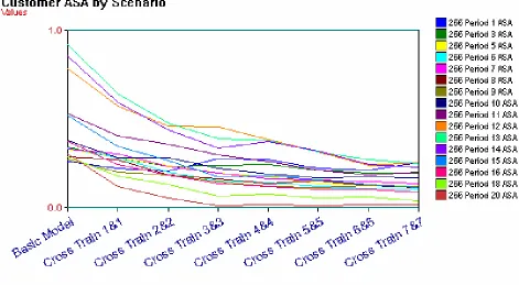
Figure 23: Customer ASA by Scenario ... 52
Figure 24: Normal Quantile Plots of Responses... 54
Figure 25: Period 3 ASA Least Squares Regression Model Results ... 55
Figure 26: Period 3 ASA Least Squares Regression Model Results ... 56
Figure 27: Period 7 ASA Least Squares Regression Model Results ... 57
viii
Figure 29: Period 10 ASA Least Squares Regression Model Results ... 59
Figure 30: Period 10 ASA Least Squares Regression Model Results ... 60
Figure 31: Period 13 ASA Least Squares Regression Model Results ... 61
Figure 32: Period 13 ASA Least Squares Regression Model Results ... 62
Figure 33: Period 17 ASA Least Squares Regression Model Results ... 63
Figure 34: Period 17 ASA Least Squares Regression Model Results ... 64
Figure 35: Number of Claims Out Least Squares Regression Model Results... 65
Figure 36: Number of Claims Out Least Squares Regression Model Results... 66
Figure 37: ASA Results of Scheduling versus No Scheduling... 71
Figure 38: Customer ASA with Cross-Training One Calls and One Claims Agent Along with Improved Scheduling... 73
Figure 39: Customer ASA with Cross-Training Two Calls and Two Claims Agents Along with Improved Scheduling... 74
Figure 40: Customer ASA with Cross-Training Three Calls and Three Claims Agents Along with Improved Scheduling... 75
Figure 41: Customer ASA with Cross-Training Four Calls and Four Claims Agents Along with Improved Scheduling... 75
Figure 42: Customer ASA with Cross-Training Five Calls and Five Claims Agents Along with Improved Scheduling... 76
Figure 43: Customer ASA with Cross-Training Six Calls and Six Claims Agents Along with Improved Scheduling... 76
ix
Glossary
258: The Provider skill
262: The Employee skill
263: The Broker skill
264: The Provider Benefits& Eligibility skill
266: The Customer skill
ASA: The average speed of answer for all calls answered within a half-hour period of the day
ACD Calls: The number of calls answered within a half-hour period of the day
ACD Time: The average waiting time for all calls in a half-hour period of the day
ACW Time: The average time the answering representative spends in wrap directly after a call completes
Confidence Intervals: All confidence intervals are 95% confidence intervals
Erlang C: A queuing formula developed by A.K. Erlang in 1917; used to determine the number of resources needed in queuing situations using the number of entities waiting to be served, the average service time, and a target for service level or ASA(Cleveland and Julia Mayben 1997).
Lower CI: The lower 95% confidence limits generated from the Arena Category Overview
Split/Skill: A VRU grouping or routing; also referred to by “skill”
SL: Service level; the percent of calls answered within a target time period
Upper CI: The upper 95% confidence limits generated from the Arena Category Overview
1
1.
Introduction
1.1
Problem Description
This thesis will attempt to demonstrate, using a trace simulation, the benefits of cross-functionality and scheduling in a large HMO call center at an anonymous for-profit health insurance agency in the United States. The call center has approximately 70 agents (depending on time period), each of which are assigned to handle different types of calls. Calls are divided into categories (known as split/skills) by a Voice-Response Unit (VRU) and fall into the following groups: Provider, Provider Benefits and Eligibility (B&E), Employee, Broker, and Customer. Employee calls are handled by specially trained agents because of privacy issues. Broker calls are also handled by specially trained agents because brokers are a direct source of revenue for the company. All agents handle Customer calls and almost all handle Provider and Provider B&E. In other words, each agent has a set of skills they are assigned to handle. See Figure 1 for an illustration of the call arrival and handling process.
Figure 1 Assignment of Calls
CallArrives
Call seizes a trunk line
Cust 266
Prov 258
Prov B&E
Emp 262
Brok 263 Call goes to appropriate queue
2
The HMO group has two divisions: the call center division and the claims processing
division. The associates that handle claims have comparable salaries and skill levels to those that handle calls. However, none of the claims associates are trained to take calls and none of the calls agents are trained to process claims, i.e. HMO is not
cross-functional. There is currently no scheduling tool in place; call center agents are assigned lunch times, but there appears to be little monitoring of agent activity to see that they take their lunches during their scheduled time. The capability to monitor this activity exists through a software package called CentreVu Supervisor, which reports what state associates are currently logged in. Its accuracy is limited because associates are
responsible for accurately reporting their state when they are not taking a call. The lunch times assigned are based on what has worked best in the managers’ experiences; they are not based in any calculated fashion on forecasted call volumes. As a result, their service level plummets midday and management frequently requests permission to hire more associates to alleviate the midday crisis period.
3
used to drive the arrival process, call answering process, abandons, and statistics
collection.
At this company, ASA is used as a service/performance measurement. However,
Cleveland and Mayben (1997)show that a better measurement is the percent of calls (X) that are answered within Y seconds. This measurement is what will be referred to as service level. For example, an 80/20 service level is 80% of calls answered within 20 seconds. A secondary service objective is to serve the caller’s needs in the shortest time, measured in CentreVu by ACD Time.
Because ASA time is calculated from the calls that get answered only and not the calls that abandon, abandons will be completely ignored in the calculation of ASA in the model. The model will, therefore, be verified by looking at ASA data. There is also data available on SL calculated using 30 seconds as the base. This data became available on 5/5/2003, so it will also be used to verify the model. However, the SL data does include abandons when calculating the statistic. To reflect this discrepancy, abandons were included in the model by creating entities called “Abandon” whose only job is to update the service level statistics collection variables. Because ASA can overestimate how long most people wait and SL hides instances when people wait much longer than 30 seconds, it is desirable to integrate the two statistics in the validation process. However, as will be explained in Chapter 4, it was not possible given the time constraints on this project to match the two statistics as closely as had been preferred. It was possible to obtain a fit that closely matched the shape of both graphs, but not the volume.
4
Agents start work at half-hour intervals from 8:00am to 9:30am and go until 4:30pm to
6:00pm, respectively. In some other call centers agents are assigned two 15-minute breaks, but in this particular call center they take short breaks (restroom, water, personal phone calls, etc.) when needed and their two breaks are added to their lunch time; this way, they can take a full hour lunch instead of a 30-minute lunch, which would be the case with scheduled 15-minute breaks. To account for such small breaks as well as absences, the number of agents was reduced by approximately 20%, similar to what was done in Pichitlamken, et al (2003). The usual amount is 68-70 agents. Using 4 months worth of login data (records of every time an agent logs into or out of the system and the date and the unique agent number) from April 2003 to July 2003, the number of agents found to be absent each day on average during a given month was approximately 13-19%. Because the months used are the warmer, more traveled months, 15% was chosen, totaling a 35% reduction in staff. Hence, the simulation model will use 44 full-time agents instead of 70.
In the data fitting process it was discovered that an equivalent reduction in the later periods of the day resulted in a high ASA. To remedy this, several part-time ‘agents’ were added; they are active only for the last few periods of the day. In fitting the data for the Employee and Broker skills, several resources were added that were only scheduled for various short parts of the day. In addition, because the resources in the model are much more efficient than real-life resources and adding or subtracting one from the list of available resources has such a large effect on the ASA and SL in the model, 6 of the regularly scheduled (full-time equivalent or FTE) resources were given failures to reduce their availability. Many of the added part-time Employee and Broker resources were given failures as well. Not accounting for lost time due to failures, the total number of FTEs in the model is approximately 48.
5
quarter-hour or half-hour intervals according to call needs, as opposed to “best-guess”
assignments by management.
The simulation will model the current situation using the data available and evaluate staffing costs and the level of customer service in terms of service level. The model will be modified to include cross-training (cross-functionality) and scheduling, with costs and service levels re-evaluated. The model is built on the Rockwell Software Arena version 7.01 (Copyright © 2002-2003 Rockwell Software, Inc.) platform. Note that the terms ‘interval’ and ‘period’ are used interchangeably throughout this paper.
1.2
Objectives
1. Examine the effects of cross-training between claims and calls:
a. What is the cost of cross-training versus the current setup, as measured by service levels and monetarily through staffing costs?
b. What is the effect of cross-training on ASA?
c. Given the salary increase and training cost of a cross-functional associate, as well as the possible service level increase resulting from cross-training, what is the ideal percentage of staff that should be cross-functional? Is this number different for the claims and calls teams?
d. How does cross-training affect the number of associates needed to staff the call center?
2. Determine the effect of scheduling breaks and lunches based on call volumes and of monitoring schedule adherence:
a. How is ASA affected?
6
1.3
Approach to Analysis
The model is initially built to accurately represent the current situation in the call center. For comparison basis, current ASA and current service levels are recorded. Cross-training is added to the model and these measurements are retaken. The current schedules are modified by changing one resource schedule at a time in an attempt to smooth the ASA curve. Each change is evaluated both separately implemented and simultaneously implemented. Employee satisfaction is evaluated using literature available in similar situations.
7
2.
Literature Review
As call center technology advances and call centers become more complex, there is a growing need for more accurate workforce management (WFM) systems. The traditional approach to call center management has been Erlang C calculations and experience-based, rather than numbers-experience-based, decision-making. Because, according to Vijay Mehrotra and David Profozich (1997) as well as Brad Cleveland and Julia Mayben (1997), many of the assumptions involved in Erlang C calculations are no longer valid, more attention has been given in the last decade to call center modeling approaches. Queuing and simulation research related to call center environments has given insight into scheduling and resource management as well as input analysis. Information on cross-training in the literature is limited, but there have been several papers outlining the usefulness of simulation in call centers and providing detailed case studies of call center simulations.
2.1
Erlang C: The Traditional Approach to Call Center Management
Brad Cleveland and Julia Mayben discuss the properties of Erlang C that make it a tool that should not be heavily relied upon. The Erlang C, or Erlang delay, model was developed in 1917 by A.K. Erlang (p. 85). It is a queuing formula developed in 1917 used to determine the number of resources needed; its applications span a variety of industries and circumstances, but in the call center environment it is used to determine resource needs to meet given service level or ASA targets. In queuing theory
8 , ) 1 ( ! ! ) 1 ( ! ) , ( 1 0 ρ ρ − + − =
∑
− − s a k a s a a s C s s k k s where ≥ < = s a if s a if s a 1 ρAccording to Cleveland and Mayben, the formula assumes that there are no abandons and that any calls that would have been lost in the real world are actually delayed until they are answered. It also assumes that there is infinite trunking capacity and that no callers will have busy signals; in the case of the call center being studied by this thesis, this assumption holds fairly true with the real system, but it is certainly not true in all call centers.
Because of these assumptions, it is a fairly accurate predictor when service level is good and there are few abandons and busy signals. However, it can overestimate staffing needs during busier periods. In addition, Cleveland and Mayben also state that Erlang C assumes that arrival traffic does not increase or decrease beyond random fluctuation within the time period. It also assumes that there are a fixed number of staff handling calls throughout the time period and that all agents within a group can handle all calls routed to the group. In the call center being studied, not all agents can handle all calls that come in, so Erlang C is not entirely applicable. Assuming that there are a fixed number of agents available also means that Erlang C cannot be used to study the effects of cross-training since cross-training is based on altering staffing levels continuously to efficiently meet demand. In complex call centers, these two assumptions are often not met and so Erlang C can seriously overestimate resource needs.
2.2
Simulation in Call Centers
9 inputs and outputs. Klungle (1997) adds that skills-based routing has added a large
amount of complexity to call centers and has made Erlang C obsolete. Usage of Erlang C models in a complex call center will often result in overstaffing. Because of the ability of simulation to account for all aspects of a call center, Klungle argues that simulation is the “best alternative” in call center modeling. Klungle (1999) goes on to describe his
experiences in simulating the AAA Michigan claims call center. His performance measures are service level, average speed of answer, agent utilization, abandonment rate, average length of call, and percent of calls answered without waiting. A shortest
processing time rule for call routing was shown to improve queue length, average waiting time, and abandonment rate when compared to the traditional routing approach of
grouping by functional type.
Bapat and Pruitte (1998) provide a detailed description of the benefits of simulation in call centers by comparing the advantages and disadvantages to those of traditional call center management approaches. To add to Klungle’s (1997) and Mehrotra’s (1997) complaints about Erlang calculations causing overstaffing, Bapat and Pruitte point out that “studies have...shown that 60% to 70% of the costs in call centers today are associated with staffing and human resources.” As a result, WFMs that use Erlang to provide scheduling recommendations are limited in effectiveness; the growing industry trend in WFM systems is to include simulation tools. According to Bapat and Pruitte, the issues faced by call centers today that can be completely addressed by simulation
techniques include:
• Efficient call handling processes
• Service level
• Skill-based routing
• Simultaneous queuing
• Priority queuing
• Agent preferences and proficiencies
10 Tanir and Booth (1999) agree with these issues and demonstrate the effectiveness of
simulation by modeling the complete customer experience in a Bell Canada call center. To limit the granularity of the data, they make the following assumptions:
• The workforce is 50% of the real one since the model does not capture training times, vacation, differences in competency level of agents, and managerial time.
• Financial input is limited to an average hourly wage for agents
• Initial call volumes are based ACD data collected at half-hour intervals They use a top-down modeling approach by first identifying the high-level processes, then adding the lower-level ones as the model develops. By adjusting the size of the workforce, they showed that a lack of resources at key times in the day can be
detrimental to the daily service level. This thesis will attempt to show that this sensitivity can be minimized by proper resource scheduling and cross-training, making more agents available at the busiest parts of the day.
Another important example of call center simulation uses recent research done in the area of input analysis by Avramidis, et al (2003). Pichitlamken, et al (2003) model a call center with inbound and outbound traffic and two types of agents: inbound-only and blend. Their objective is to meet a service level requirement. The challenges they outline are similar to those faced in the model of this paper:
• The format of the data available is in 30 minute interval aggregates
• Arrival rates vary from day to day and within days
• Only the maximum patience time is observed for those who abandon, not for those who are served
• Actual agent availability is difficult to determine due to short breaks, absenteeism, personal calls, etc. They account for this difficulty using a global reduction or the workforce by a fixed percentage (10% to 15%), similar to the approach taken by Tanir and Booth (1999).
11
2.3
Scheduling and Resource Management
Because so much of a call center’s cost is in staff needs, much research has been done on agent staffing levels, especially using queuing models. Andrews and Parsons (1993) consider a different method of optimization by focusing on economic considerations rather than meeting a set service level objective. Because their objective was slightly different than the traditional approach, they considered trunk-usage charges as a cost of waiting in addition to the average hourly wage of agents. In contrast, Koole and Sluis (2002) consider a shift scheduling problem where the goal is to meet an overall service level objective as opposed to scheduling to meet a service level at every interval.
Askin and Harker (2001;2003) consider more than just human resources. The
dependency between difference resources in inbound call centers is investigated in Askin and Harker (2001). A queuing model is developed for both a loss system and a system with reneges that is the “first in the literature to capture the impact of shared information processing resources on phone center performance.” The model presented is useful in determining when it is more cost effective to increase capacity through hiring agents or through investing in an information system upgrade. Following the lead of Andrews and Parsons (1993), Askin and Harker (2003) go on to model a system with reneging where optimality is defined as maximizing profits, not meeting a pre-defined service level. The objective is to find the optimal number of servers to be allocated to different call types when there is a common shared limited resource. The resources they consider in addition to human agents are VRUs (Voice Response Units) and information technology
12
2.4
Cross-Training and Skill Transfer
Cross-training agents carries with it certain considerations for the human factor. The model does not account for the initial training process as it depicts the long-run effect of cross-training. In addition, in determining the length and approach to training, one must examine the nature of the new skills in relation to skills already possessed.
Information in the literature on cross-training in a call center environment is extremely limited, but Leshner and Browne (1993) outline the benefits of cross-training in the insurance industry:
• Increased productivity (average of 20%)
• Shifting of staff to support growth
• Improved customer service
• Increased employee morale
• Increased flexibility
• Provides career development opportunities for employees
• Culture becomes more progressive
13 Because processing claims and taking calls may have certain skill requirements in
common, it is important to examine the possible interaction or lack of interaction of skills necessary to perform each task. In general, according to Swezey and Llaneras (1997), the learning process follows a power function, i.e.“performance improves rapidly early in practice, but soon approaches a state of diminishing returns where each additional increment in performance requires longer and longer practice intervals.” Additionally, “easy tasks often lead to ceiling effects, while excessively difficult tasks often
demonstrate an insensitivity to practice.” The difficulty level of learning a new task is affected by “…meaningfulness, concreteness, familiarity, and associations with other information in the memory store.” The difficulty of cross-training will be affected by the level of association, similarity, and interaction between the two tasks. Hence, the training program used to train new associates in either task may not be suitable for associates who are already practiced in the other in that if there is likely no negative transfer, it may need to be abbreviated.
2.5
Input Analysis
Traditionally, arrival processes for incoming call centers have been modeled using a general Poisson process. Recently, however, this standard has been studied more closely and shown to be significantly inaccurate. A queuing model of a small bank was created by Brown, et al. (2002) for the purpose of studying arrival and service time distributions. The group had access to one year’s worth of detailed call-by-call data. Analysis showed that arrivals are best described by an inhomogeneous Poisson process and that service times (talk times) are most accurately modeled using a lognormal distribution. They also discovered that arrivals and service times are positively correlated as a function of the time of day, i.e. the busier it gets, the longer the service times become. A possible
14 More recently, Avramidis, et al. (2003) executed a similar study with a focus on arrival patterns and intra-day, not day-to-day correlations. They outline the following properties of arrival processes:
• P1: The total number of calls in a day “has overdispersion relative to the Poisson distribution”
• P2: “The arrival rate varies considerably with the time of day”
• P3: “There is a strong positive association…between arrival counts in a time partition of a day”
• P4: “There is a significant dependency between arrival counts on successive days”
They create three models that capture P1 through P3. Model M1 uses a doubly stochastic Poisson process for arrivals. Model M2 has a more flexible covariance matrix than model M1 and model M3 has the greatest flexibility in induced moments. Their case study of a Bell Canada call center using these models shows that “simulation-based call center performance measurement is sensitive to the arrival-process model.”
2.6
Employee Satisfaction
In addition to training considerations, cross-training also compels one to bear in mind the effect on employee satisfaction. The model built assumes that there will be no change in the behavior of the employees. Because, say Kalimo, et al (1997), job satisfaction is an important factor in absenteeism and turnover as well as (it can be assumed) productivity, it should be a consideration in deciding whether or not to cross-train agents.
15 and career development is one way to decrease psychological distress in associates.
16
3.
Model Description
This chapter will describe in detail the basic model, the model with cross-training, the model with scheduling, and the model with both cross-training and scheduling. Chapter 4 deals with the analysis of these models. The replication length is 236 days, the number of days available in the data for the extended hours. Statistics and the system are
initialized between replications and there is no warm-up period.
The general modeling approach used is a trace-style simulation with some modifications. Using a trace simulation as a basis was chosen to attempt to model what actually
happened during the year from which the data was taken as closely as possible. Because the arrivals are not a regular Poisson Process and the service times are not exponential, a technique that would allow for the specification of such details was needed. Because of the nature of the data, an exact trace simulation could not be used. The data being given in half-hour interval summaries requires interpretation of what happened in the system on a lower level during each of those half-hour periods. What is not known from the data is the exact arrival time of each call, the exact wait time of each call, the talk time of the calls, and the time the agent spent in wrap. Instead, what is known is the sum of the calls answered in a period and the average waiting, talk, and wrap times. Therefore the
simulation is “trace-like” in that it uses the data given directly, but it is not completely a trace simulation since variability and randomness are introduced in the arrival process, talk times, and wrap times. This randomness also necessitates replications to reduce the standard deviation of the performance measures- primarily ASA but also SL.
17 in wrap. They also read the current period of the day (1=8:00am-8:30am,
2=9:00am-9:30am, etc.) and the current day (1=Monday, 2=Tuesday, etc.). The value of each data point gathered is stored in an attribute or a variable for later use. In the case of the regular call arrival processes, the control entity loops for the rest of the 30 minutes by passing through a delay block and a separate block to simulate the interarrival times and arrivals of calls, respectively. At the end of the period, they are sent through some statistics collection modules and are disposed. The control entity used to gather information about day and time simply loops continuously for the duration of the simulation.
3.1
Data Collected and Use of Data
The data collected has been briefly outlined in the introduction. Before using the data in the modeling or validation, much of it had to be gleaned and manipulated. This section will discuss the preparation of the data as well as how the data is used as input in the model.
3.1.1 Preparation of Data
Apart from the five described earlier, the original data came with several Split/Skills that were not highly used (in fact most had no call volume) and one Split/Skill that was used enough that it needed to be included in the data. An employee at the company
recommended that it be included in the Employee group. To combine the skills, the ACD Calls and Abandoned Calls data points were summed for each separate interval. The ASA was multiplied by the respective ACD Calls datum; the two quantities were added and the sum was divided by the sum of the ACD Calls for both skills to obtain an overall ASA. A similar approach was taken for Average Abandon Time, ACD Time, and ACW Time. The skills that were insignificant were deleted from the data.
18 8:00am-8:30am corresponded to period 1, 8:30am-9:00am to period 2, etc. Using the
data functions in Microsoft Excel, the data was interpreted as the day of the week and also assigned a number in a new column. Monday corresponded to day 1, Tuesday to day 2, etc. The data was then divided by skill so that each skill had a separate spreadsheet. The day and interval did not always align for all skills; occasionally intervals would be missing and sometimes there were records for intervals prior to 8:00am or past 6:30pm. When records needed to be added for missing intervals, it was assumed that call volume was zero. Any intervals not between 8:00am and 6:30pm were deleted from the data. The data was cleaned up so that the date and period lined up for all five skills. The file that the data is read from in the model was created from this gleaned and organized database.
The login data used as a starting point for agent skill assignments fitting was analyzed by querying the data for a short time interval (one month) and for unique login identification numbers. Then the number of observations of unique login IDs was examined; if an ID was only observed a few times (as opposed to several dozen times), it was likely to be a manager logging in to make changes in the system (according to an employee at the company) and was disregarded. After removing these ‘manager’ ID records from the data, the login data was also used to determine absence rates; this analysis was performed in a similar fashion using Microsoft Access to query the data by day to get the total number of IDs that logged in each day.
3.1.2 Use of Data in Model
As described in the introduction, much of the data was used to find a starting place for the data fitting process. The schedule that was obtained from the HMO manager was used directly initially but had to be modified during the verification process to fit the data. Also, the login data was used to find a good starting place for the distribution of agent skills but was, again, modified during the verification process to fit the data. The rest of the data was used directly either in verification (ASA and SL averages) or in the
19 The model reads data from the following categories:
• ACD Calls (number of calls answered per period)
• Average ACD Time (average talk time)
• Average ACW Time (average time spent in Wrap)
• Abandoned Calls
• Average Abandon Time (average time until call abandons)
• Day
• Interval
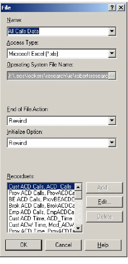
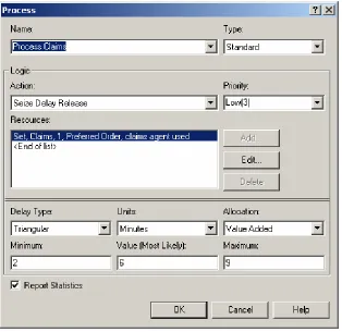
It utilizes the File module and ReadWrite module in Arena. The data is read from a Microsoft Excel spreadsheet with named ranges. The File module is shown below in Figure 4. The file rewinds when it reaches the end, which occurs at the end of each replication. The Recordsets are the named ranges in the Excel file. Each ReadWrite module assigns an attribute to the entity with a value of the data point read.
20
Figure 2 File Module
3.2
Overview of Basic Model
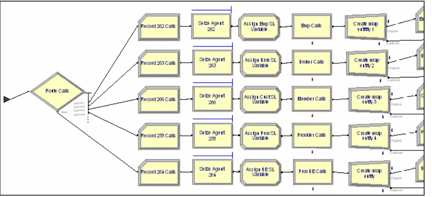
21
Figure 3 Submodel Flowchart
22
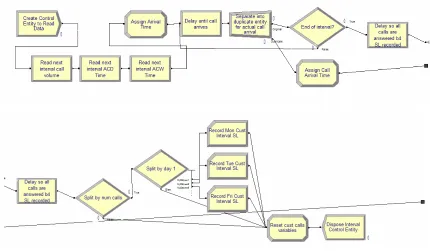
3.2.1 Arrival Process
Since each arrival process is the same for all skills, this description and any screenshots provided will be from the Customer 266 split/skill. Below (Figure 5) is a view of the arrival process flowchart. It is too long to fit in one screenshot; the right half is below the left half.
Figure 5 Call Arrival Flowchart
23
Figure 6 Control Entity Create Module
The ‘Arrival Time’ attribute is used to keep track of the time that the current half-hour interval began. The MyInterval attribute is used for statistics collection to refer to the interval during which the entity actually arrived; the current period may be a later period that the arrival period. The Control Entity then enters a delay block where it is delayed for a period of time determined by the Expression ‘Interarrival Times’ (Figure 7).
24 Interarrival Times is a row of the Expression spreadsheet module and is the following
expression:
(ACD Calls = = 0)*30 + (ACD Calls <>0) *EXP((30/(ACD Calls + 0.000001))). If the value of the attribute ‘ACD Calls’ is equal to zero, the first set of parentheses will return a value of 1; hence, the entity will be delayed 30 minutes, the full interval length. Otherwise, the first set of parentheses will return a value of 0 and the second set of parentheses will return a value of 1. In that case, the entity will be delayed an exponential amount of time with mean 30/(ACD Calls). Adding a small number is necessary for the compiler not to read a divide-by-zero when ‘ACD Calls’ is zero. Delaying a simple exponential length of time is not precisely correct due to the fact that some entities that should arrive in the interval in which the parent Control Entity was created will arrive in the following interval with a delay length based on the previous intervals call volume. However this approximation does not appear to distort the representation of the actual arrivals.
After delaying the length of the interarrival time, the Control Entity is sent to a Separate module (named ‘Separate into duplicate entity for actual call arrival’). The duplicate entity can be thought of as the actual call that has arrived. It is the entity that will go on to the ‘Process Calls’ submodel. This entity has inherited all of the attributes of the parent Control Entity. It moves on to an Assign module where it is assigned its own attribute ‘arrivalTime’ with a value of TNOW. This attribute is used to reference the arrival of the actual call. The call entity is also assigned the attribute ‘MyInterval’ with a value of ‘Period’ since its arrival period may be different from its parent. Similarly, it is assigned the attribute ‘MyDay’ with a value of the variable Current Day. A couple of variables are also assigned here for statistics collection purposes; these assignments will be described later in Section 3.2.6.
25 calls per period’ variable in both the ‘Assign Call Arrival Time’ and ‘Reset cust calls
variable’ Assign modules; and to delay the recording of the interval SL until any entities that arrived in the interval being recorded have either completed their queuing or have waited longer than 30 seconds. Calls are then sent to two Decide modules. The first (‘Split by num calls’) is for statistics collection purposes and send calls to the next Decide module and hence to a Record Module only if the number of calls in the interval that just ended is greater than zero. The Record module (Figure 9) collects interval service level statistics by day (the second Decide module routes to the correct Record module based on the value of ‘MyDay’) and the Assign module resets two variables used to collect SL statistics back to zero. This statistics collection process will be described in more detail in Section 3.2.6.
Figure 8 End of Interval Decide Module
26 The original Control Entity moves back to the ‘Delay until call arrives’ module after
leaving the Separate module and repeats the process. Once the duplicate entity leaves the ‘Assign Call Arrival Time’ module, it completes the arrival process and moves on to the ‘Process Calls’ submodel.
3.2.2 Time Period Counter
The Time Period Counter (Figure 10) section of the model is completely separate from the rest of the model. The purpose is to keep track of the current day (1 = Monday, 2 = Tuesday, etc.) and the current time interval (1 = 8:00am-8:30am, 2 = 8:30am-9:00am, etc.). The counter entity is created only once per replication at the start of the run.
Figure 10 Time Period Counter Flowchart
27
Figure 11 End of Day Decide Module
3.2.3 Process of Answering Calls
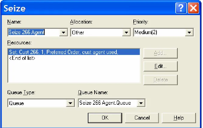
When calls arrive in the Process Calls submodel, they are immediately routed by call type through a Decide module (Figure 12). So that queue times can be recorded for both ASA statistics and SL statistics, the seize and delay processes are separated. Because of the wrap-up process, the release of the resource is also separate.
28 After the decide module, the call enters the Seize block (Figure 13) where it will wait for an available agent. It seizes a resource from the appropriate resource set (in this case the set ‘Cust 266’, which is the set of agents that can answer customer calls) and gives the resource an attribute to designate which resource from the set has been used so it can release the correct resource later on. The resource selection rule is not tremendously important since there is no difference in skill level in the model between agents, but Preferred Order was chosen so that the part time agents would be used the least and so that in the model with cross-training the cross-trained claims agents would be used last. At the company, calls are routed to the agent that has been available the longest. It is possible to model this selection criteria, but not practical since agents are known to manipulate the system by going into non-call busy modes to shorten their availability time.
Figure 13 Queuing of Calls in Seize Agent Module
29 JOHN(1.354,.887,.58*(ACD Time),.87*(ACD Time),10)
The expression was found by assuming that talk times can be approximated by a
JohnsonSB distribution (since no actual call time data was available- only averages over 30-minute intervals- an assumption as to the shape of the distribution had to be made). In the expression, ‘ACD Time’ refers to the attribute assigned to the Control Entity that gives the current interval’s average talk time. The last parameter in the distribution is the random number stream used. To derive the Johnson distribution parameters, basic assumptions were made about the minimum, maximum, and mode. The program VIM (Version 2.0, Stephen Roberts, Lijun Wang) was used to determine the shape parameters that would result from this minimum, maximum, and mode combination and to graph the CDF and PDF (Figure 15). After several runs of the simulation (while using VIM to modify the mode or median) to improve the fit from this starting point, the minimum, maximum, and mode were modified to produce the above distribution.
30
Figure 15 VIM PDF and CDF
31 as ‘ACD Times’, the only difference being that it uses the attribute ‘ACD Time’ assigned in the arrival process submodel. Below is the Expression:
JOHN(1.354,.887,.58*(ACW Time),.87*(ACW Time),12)
Upon completion of the wrap process, the duplicate entity moves to a record block where the wrap delay time is recorded and is then disposed. This completes the flowchart of calls through the system.
32
3.2.4 Abandons Arrival and Processing
As with Section 3.2.3, any screenshots in this section will be taken from the Customer 266 Split/Skill. The abandons arrival and processing is the same for all Split/Skills. Below (Figure 17) is a view of the entire abandons arrival and processing flowchart.
Figure 17 Abandons Arrival and Processing Flowchart
33
Figure 18 Abandons Separate Module
3.2.5 Employee Skill Sets, Schedules, and Failures
There is one resource for every agent and one schedule as well. For example, agent Jane Doe would be a single resource of maximum capacity one and corresponding
individualized schedule ‘Jane Doe sched’. The schedule rule used for all resources is Ignore, meaning that when an agent is scheduled to go on break or off shift, he or she finishes the call they are currently processing before starting the change in the schedule. In addition, the time during which the capacity is zero starts when it is scheduled to start rather than when the resource actually begins the schedule change, as described in
34 downtime ranges from 0 to 30 minutes over the periods. A list of the resource names and schedules used is provided in the appendix in Table A1. Some of the schedules are not the typical 8.5 hour day with a one-hour lunch. It was necessary to modify a couple of the schedules to better fit the data. Below Table A1 is a table of the resource skill assignments; this is in Table A2. The resources in bold have failures assigned to them.
There are five employee skills sets, one for each Split/Skill. They are ‘Cust 266’, ‘Prov 258’, ‘Prov BE 264’, ‘Brok 263’, and ‘Emp 262’. Each of these sets is of the type Resource set. To determine the composition of each of these sets, one month worth of agent login data was analyzed to determine what percentage of all agents logged in to each skill. It was found that each agent that logged into the system had logged into the Customer 266 skill. Approximately 96% of agents logged into the Provider 258 skill, 94% into the Provider B&E 264 skill, 37% into the Broker 263 skill, and 26% into the Employee 262 skill. However, during the validation process it was found that this distribution needed to be modified to fit the data. In the process, some part-time resources were added to the employee and broker skill sets only. The new percentages are:
• Customer: 94%
• Provider: 65%
• Provider B&E: 78%
• Broker: 48%
• Employee: 41%
3.2.6 Statistics Collection
35 verification purposes only. Outside of resource states, statistics will be described in the order in which they appear in the model.
Service level statistics are the most complicated statistics collected and the process begins in the arrival submodel. After the Control Entity separates in the Separate module called ‘Separate into duplicate entity for actual call arrival’, it enters an Assign module where it updates a variable used in the SL statistic (Figure 19). In the case of the Customer 266 skill the variable is called ‘cust calls per pd’ and is a 21-dimensional array variable. This assignment increments by one the index of the variable corresponding to the period in which the call arrived, represented by the attribute ‘MyInterval’.
Figure 19 A Service Level Variable Assignment
The ‘Split by day’ Decide module routes calls to Record modules only for Mondays, Tuesdays, and Fridays. These three days were chosen because, according to Cleveland and Mayben, Monday tends to be day of highest call volume in most inbound call centers, Friday tends to be the slowest day, and Tuesdays are generally similar to
Wednesdays and Thursdays. As shown in Figure 20, the Record module logs the percent of calls answered within thirty seconds for the previous interval as given by the
expression:
36
Figure 20 Recording of the ASA Statistic
It has already been described how the denominator of the above expression is arrived at. The numerator is a similar 21-dimensional variable that is updated in the ‘Process Calls’ submodel just after the caller seizes an agent. In the ‘Assign Cust SL Variable’ module, the index corresponding to ‘MyInterval’ of the variable ‘cust calls answered in 30s’ is updated to the following value:
arrivalTime )<= .5)*(cust calls answered in 30s(MyInterval)+1) + ((tnow-arrivalTime) > 0.5)*(cust calls answered in 30s(MyInterval))
In words, the above expression will increment the variable by one if the caller has waited no more than 0.5 minutes; otherwise it will remain the value it is currently. After passing through the Record module, the call goes to an Assign module where these two variables are reset to 0 in preparation for the next day’s SL computation.
There is a tally statistic for each combination of skill, period, and day (Monday, Tuesday, or Friday). Sets are used to record into the tally statistic corresponding to the interval being recorded. For example, ‘Mon Cust Interval SL’ is a tally set composed of the 21 tally statistics representing the Monday Customer SL for each of the 21 intervals. Therefore, in Figure 20 ‘MyInterval’ provides the set index of ‘Mon Cust Interval SL’ in which to record the computed interval SL.
37 variable. The ‘cust calls answered in 30s’ variable is updated in a similar fashion as in
the arrivals submodel. In this case the expression is:
((Aban Time )<= .5)*(cust calls answered in 30s(MyInterval)+1) + ((Aban Time) > 0.5)*(cust calls answered in 30s(MyInterval))
The result is the same as above, the only difference is that the entity is previously assigned a time to wait until abandoning. For simplicity’s sake, this time is equal to average time to abandon from the data. If this time is not greater than thirty seconds, ‘cust calls answered in 30s’ is incremented by one.
The next statistic collected is the number of calls by skill. After being routed by skill type, the calls pass through a Record module called ‘Record 266 calls’ which counts by one and records into a Counter set. There are five sets, one for each skill, and they are composed of 21 Counter statistics corresponding to each period.
ASA is recorded just after the resource is seized by a call entity. Like SL, it is recorded into a tally set composed of 21 ASA tally statistics, each representing a period for that particular skill. For the Customer skill, the tallies are named ‘266 Period 1 ASA’, ‘266 Period 2 ASA’, etc. and the tally set is called ‘266 ASA’. The Customer Record module (Figure 20) uses ‘MyInterval’ as the set index and records into the tally set ‘266 ASA’. The value it records is the length of the time interval from ‘arrivalTime’ to TNOW, the current simulation time.
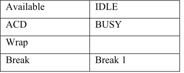
38 Finally, the StateSet spreadsheet module is used to create a set of resource states agents enter into. The purpose is to be able to view Frequency statistics to see that the time spent in each state or failure is what is expected and seems to fit the real world
proportions. The four states and their corresponding system state, when applicable, or failure name are given in Table 1.
Available IDLE ACD BUSY Wrap
Break Break 1
Table 1 StateSet 'Agent States'
3.3
Description of Model with Cross-Training
The model that includes cross-training has only a couple of key differences from the basic model. First, it has a new resource(s) whose primary function is to process claims. In addition, one or more of the current calls resources become cross-trained. This
39
Figure 21 Claims Submodel Flowchart
Claims are created once a day with a quantity of 1000. This creation process was chosen so that the number of entities in the system did not grow out of control but there were always claims waiting to be processed. It has been assumed that there is always claims work to be done. The claims Process module (Figure 22) uses a Priority of ‘Low’ for claims. This assignment assures that when call volumes are high enough to warrant the assistance of the claims representatives the claims are put aside until call handling
40
Figure 22 Claims Submodel Flowchart
The analysis was performed with the cross-training of between one and seven of both calls and claims agents. The following calls agents were added to the claims resource Set in the following order:
1. Resource 24 2. Resource 22 3. Resource 16 4. Resource 34 5. Resource 17 6. Resource 23 7. Resource 27
41 1. 8:00am to 4:30pm with lunch at 11:00am
2. 8:30am to 5:00pm with lunch at 12:00pm 3. 9:00am to 5:30pm with lunch at 1:00pm 4. 9:30am to 6:00pm with lunch at 2:00pm 5. 8:00am to 4:30pm with lunch at 11:00am 6. 8:30am to 5:00pm with lunch at 12:00pm 7. 9:00am to 5:30pm with lunch at 1:00pm
These schedules were chosen to distribute as evenly as possible the shifts and lunch breaks, with a focus on the earlier shifts (in the actual environment there seems to be a preference for the earlier shifts).
3.4
Description of Model with Scheduling
The scheduling model is only different in its distribution of schedules. This distribution was found by starting with the basic HMO model and altering schedules until the ASA graph was reasonably smooth. The goal was to minimize the maximum average waiting time without changing the availability of resources (i.e. without adding any new
resources or lengthening the current schedules of resources). Table 2 below contains the list of employees whose lunch times were changed and the time that it was changed to. The results of this change are shown in Section 4.4 where they can be compared to the basic model.
Resource 3 1:30
Resource 13 1:30
Resource 22 2:30
Resource 25 1:30
Resource 29 12:30
Resource 16 11:00
Resource 24 11:00
Resource 27 11:00
Table 2 New Lunch Schedules
42
4.
Analysis
This chapter will describe the process through which the workings of the model were verified to accurately represent the real-working system as well as how the model was validated to fit the data obtained from the actual system. Various debugging capabilities in Arena were utilized to verify the model. The validation was done by changing various statistical distributions in the model, resource schedule, and resource set compositions and comparing the results to the ASA and SL from the data.
Of central importance, this chapter will detail the results of the comparison study of cross-training and scheduling versus the current system in place. The interval ASA for the Customer skill is used as a basis of comparison. For the claims model, the difference in claims output is also examined. As described in the beginning of Chapter 3, the basis of the analysis is that the simulation is a trace simulation in that several inputs are read directly from the data, but that there is variability that creates a need for replications. This variability comes from the exponential arrival process and the JohnsonSB
distribution of the talk times and wrap times (whose average values are read in from the data). Because of the variability, confidence intervals will be used to compare means between the Customer ASA results of the basic model and the Customer ASA results of the experimental model. To further examine the statistical difference between the basic Customer ASA and the ASA of the experimental model, JMP v. 5.1.1 (A BUSINESS UNIT OF SAS Copyright © 1989 - 2004 SAS Institute Inc.) was used to design an experiment to analyze the effect of cross-training on claims output and ASA.
43 The number of replications used for running the models was determined with an ASA
halfwidth of 5 seconds for the intervals 2:00pm and 2:30pm in mind (2:00pm and 2:30pm were chosen because they had the highest halfwidth in the range 8:00am to 5:00pm). Using the formula n = n0h02/h2, available in Kelton, et al (2002), with n0 = 8, h0 = 0.09,
and h = .0833, n, the number of replications needed, was found to be 9.3, which is rounded up to 10. After running the basic model with ten replications, the 95% confidence intervals were indeed reduced comfortably below five seconds.
For ease of notation, the intervals of the day will often be referenced by their period number, given in the table below (Table 3).
1 2 3 4 5 6 7 8 9 10 11 8:00am 8:30am 9:00am 9:30am 10:00am 10:30am 11:00am 11:30am 12:00pm 12:30pm 1:00pm
12 13 14 15 16 17 18 19 20 21 1:30pm 2:00pm 2:30pm 3:00pm 3:30pm 4:00pm 4:30pm 5:00pm 5:30pm 6:00pm
Table 3 Intervals of the Day
4.1
Verification
The first step in the verification was to check for accuracy of the flowchart of the model. This involved using animation to watch Control Entities enter the system and duplicate; call entities leave the Separate module and route correctly to the Call Process module; and duplicate entities enter and leave the wrap Process modules. To see that entities were being routed correctly, the Watch debugger was used to watch the ‘type’attribute. In addition, the ‘ACD Calls’ attribute was watched to see that it matched not only the data being read (this was done for the other RecordSets) but also the incrementing of the ‘calls per pd’ variable. The built-in module counts that are animated were used to see that the number of entities duplicated matched the number being disposed after the call
44 for each skill equaled the sum of the ACD calls for the data. This was checked using the counter statistics collected on the number of calls per period.
The second part of the verification process was verifying that the statistics worked the way that they were expected to. The ASA statistics collection was easy to verify since it is a fairly simple and straightforward process. To see that it was working correctly, the Watch debugger and ‘Break on Module’ was used to examine the expression ‘TNOW-arrivalTime’ upon entering the Record module in which wait time is calculated and recorded in the ASA sets. By looking at call volume and agent utilization, the expression was examined for any inconsistencies such as zero wait times followed by one or two single extremely long wait times.
The service level statistics collection verification was much more complicated. The first step was to see that the minimum and maximum values for all periods were not less than zero and not greater than one, respectively. Initially the attributes ‘MyInterval’ and ‘MyDay’ were not used. It was discovered through watching the ‘cust calls per pd’ variable and the ‘calls answered in 30s’ variable that many recordings of SL were being recorded into the period after the one in which the calls arrived. In addition, some of the SL recordings the 6:30pm period were being recorded into the 8:00am period of the following day. Adding the aforementioned attributes solved many of the problems involved in the SL statistics collection. The Delay module ‘Delay so all calls are answered b4 SL recorded’ was added after it was discovered through watching the SL variables that even with the ‘MyInterval’ attribute, some of the calls would arrive at the end of a period and wait less than thirty seconds, but not be included in the SL calculation because the period would end and the calculation would be performed before the call was actually answered.
45 glaring inconsistencies (one or more skills occasionally had extremely low or high cycle times). When these outputs appeared normal, a final run-through with the watch
expressions was done to check for any additional problems, but none have been found. The model appears to be working as expected.
4.2
Validation
The model validation process involved changing the following general aspects of the model:
• ACD Time distribution
• ACW Time distribution
• Failures uptime and downtime
• Using exponential versus uniform interarrival times
• Resource schedules
• Resource set composition
For ease of fitting, it was assumed that the ACD and ACW times would have the same distribution, where both distributions would use the respective ‘ACD Time’ or ‘ACW Time’ attribute in the distribution. A beta distribution was used initially, but then was changed to the JohnsonSB distribution. The parameters were determined by starting with a mode of ‘0.9*mean’, a min of ‘mean/1.2’, and a max of ‘mean/0.8’ and manipulating the median, mode, min, or max until a suitable fit of the ASA and SL was found for the Customer skill (Monday SL). Using exponential interarrival times seemed a better model of the real system and increased the ASA and decreased the SL.
46 The service level data available is only from approximately three months of calls, so
when broken down by interval and by day, each interval mean is calculated from one to eleven data points. Because of the restricted data availability, the data fitting was focused on the ASA. There is eleven months worth of ASA data available. Because finding the overall ASA for each interval involved some calculation (sum of ASA*ACD Calls divided by sum of ACD Calls), it was too cumbersome to calculate the ASA for each day and each interval. Therefore, the data fitting was concentrated on the ASA for each interval without day as a factor. To fit the data, the ACD/ACW Times distribution found from the first round of fitting was kept while changes were made to failures, schedules, and resource set composition. Confidence intervals reported from the Arena output were used to determine how close the fit was. The Appendix contains the graphs of the final fits of the ASA and the SL used in the basic model along with a table (Table A3) indicating the percent difference of the fit from the data for each interval.
47 in contrast with the shape of the SL from the data can be explained by the small number of data points available for each interval and each day. For a given day-interval
combination, the simulation uses about 47 observations; the data has anywhere from one to eleven observations for each day-interval combination (by skill).
Due to great difference in data availability of the ASA over the SL, the ASA was fit to the data in all 21 periods for the Customer skill and for 15 to 18 periods for the other four skills. In addition, many of the intervals that were not fit within the confidence interval were off of the data mean by less than five seconds. The SL fits are in general good in shape but are mostly too high, with the exception of a couple of the Broker and Employee days.
4.3
Analysis of Cross-Training Model versus Basic Model
This section describes the analysis of the basic model compared to the cross-training model in terms of its effect on claims output as well as Customer ASA. Detailed analysis on ASA is performed by looking at 5 of the 21 intervals.
4.3.1 Claims Output without Cross-Training
48
Claims Volume
Data 3-Jan 3-Feb 3-Mar 3-Apr 3-May 3-Jun 3-Jul 3-Aug
Days 31 28 31 30 31 30 31 31
Monthly total 44516.1 41085.2 51951.9 45541.6 47834.6 44634.6 59816.4 46124 Average Per
Day 1436.0 1467.3 1675.9 1518.1 1543.1 1487.8 1929.6 1487.9
Table 4 Claims Volume Data by Month
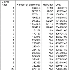
Table 5 shows the output from the simulation for the total claims volume with one to seven full-time claims agents added without cross-training. It includes the cost for 236 of employing the claims representatives at the yearly salary of $40,000 (the salary for a cross-trained representative is approximately $49200). Because the average difference between each additional claims resource has a mean of 18,909.23 with a relatively small standard deviation of 46.7, projections can be made for total claims volume over the 236 day period by adding the mean to the previous output. This projection is done for eight to twenty claims resources, as shown below. At twenty claims resources, the total projected claims output exceeds the data average 236-day output.
Claims
Reps Number of claims out Halfwidth Cost
1 18893.3 57.91 36302.70
2 37798.5 28.97 72605.40
3 56704.1 32.59 108908.10
4 75683.5 80.27 145210.80
5 94525.3 102.27 181513.50
6 113462.8 121.15 217816.20
7 132348.7 120.62 254118.90
8 151258 N/A 290421.60
9 170167 N/A 326724.30
10 189076 N/A 363027.00
11 207986 N/A 399329.70
12 226895 N/A 435632.40
13 245804 N/A 471935.10
14 264713 N/A 508237.80
15 283623 N/A 544540.50
16 302532 N/A 580843.20
17 321441 N/A 617145.90
18 340350 N/A 653448.60
19 359260 N/A 689751.30
20 378169 N/A 726054.00
49
4.3.2 Claims Output with Cross-Training
The simulation was then run with cross-training added, where the claims representatives were trained in skills 266, 258, and 264 (Customer, Provider, and Provider B&E,
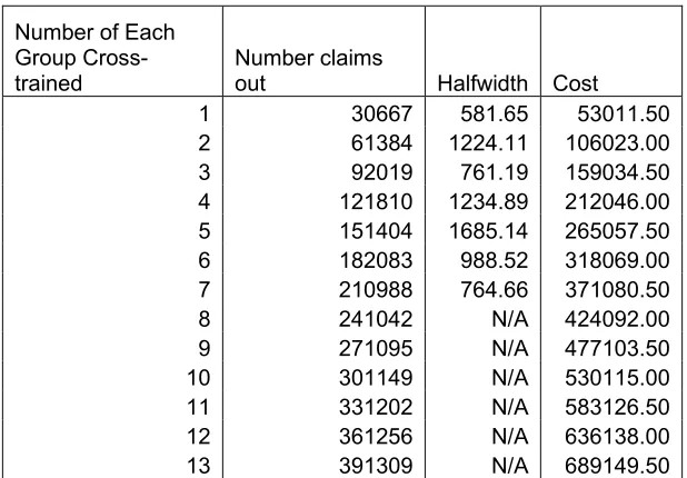
respectively). Table 6 shows the simulation output for each run with cross-training from one each of calls and claims agents to seven each. From eight to thirteen agents each, the number of claims out is projected by adding the average difference of adding one agent to each group of 30053.5 claims (with a standard deviation of 744.14) to the previous total. The cost of employing for 236 days the respective number of cross-trained calls and claims agents is also given. The calculation is based upon an estimated fully-loaded salary of $49,200.
Number of Each Group Cross-trained
Number claims
out Halfwidth Cost
1 30667 581.65 53011.50
2 61384 1224.11 106023.00
3 92019 761.19 159034.50
4 121810 1234.89 212046.00 5 151404 1685.14 265057.50
6 182083 988.52 318069.00
7 210988 764.66 371080.50
8 241042 N/A 424092.00
9 271095 N/A 477103.50
10 301149 N/A 530115.00
11 331202 N/A 583126.50
12 361256 N/A 636138.00
13 391309 N/A 689149.50
Table 6 Claims Volume Output Totals with Cross-Training
Table 6 shows that the total number of cross-trained calls agents and claims agents is 13 each to surpass the total average output from the actual data. This result involves
employing seven fewer claims agents total while cross-training 13 existing claims agents and 13 existing calls agents. The percent difference in cost is (726054.00-689149.50)/ 726054.00 = .0508, or a 5% decrease in cost from the basic model. Given the
50 decrease in cost is notable. Additionally, at this point the decrease in resource needs for the calls agents as a result of cross-training has not been factored into the cost.
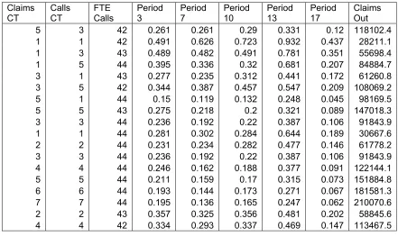
4.3.3 JMP Analysis of Cross-Training Effects on Customer ASA and Claims Output
The Appendix includes graphs of the Customer ASA for the following scenarios: one cross-training each of claims and calls agents, two cross-training each of claims and calls agents, and so on up to seven each (Figures A20-A26, respectively). Given that the company goal is to have an ASA of 30 seconds or less for each interval, it would appear that adding two cross-trained agents to each group would suffice to meet that goal. In terms of percentages, that would involve cross-training 4.167% of the calls staff and the equivalent number of the claims staff. Cross-training any more than that would likely result in overstaffing. However, there is no significant improvement in the SL from training two agents per group, as can be seen in Figure A27. With four cross-trained agents each, the Customer Monday SL shows some improvement in intervals 11:00am-12:30pm and 1:30pm-3:30pm; a graph of the SL values is shown in Figure A28.