ABSTRACT
BLAKE, SAMANTHA LYNN. Dyed Fiber Analysis towards the Development of a LC-MS Comparative Finished Fiber Database for Forensic Purposes. (Under the direction of Dr. David Hinks and Dr. David C. Muddiman).
Traditional forensic fiber analysis includes Fourier transform infrared spectroscopy,
microscopy, microspectrophotometry, and sometimes thin layer chromatography of the
extracted dye. These methods give information about the fiber type and treatment; however,
they lack molecular specificity. The introduction of liquid chromatography-mass
spectrometry analysis of the extracted dye information would provide molecular information
to the analysis and decrease the chances of incorrect fiber identifications and comparisons.
This research includes the construction of a dye proof-of-principle database containing 50
different dyes and its application to unknown dyes and degraded dyes.
The unknown dyes that were analyzed were searched against the proof-of-principle
database and correctly identified using the Agilent Qualitative Analysis B.04 software.
Another method using k-NN analysis after pretreatment of the database dyes by principle
component analysis also accurately identified unknown dyes. A selection of the dyes studied
were exposed to UV light for a defined time period then analyzed to determine the database
applicability on degraded samples. After degradation of the dye molecule due to the
exposure to UV light, enough dye was present in the fibers to get an accurate identification
from the dye database for all of the dyes studied, except for CI Acid Green 16, a
triphenyl-methane dye that is known to have poor lightfastness. This helps to validate the creation and
use of the database for forensic purposes due to the exposure of the fibers of interest to
The ability of two instrument platforms to analyze small molecules was also
compared. Color Index Disperse Yellow 42 (DY42), a high-volume disperse dye for
polyester, was used to compare the capabilities of the LTQ-Orbitrap XL and the
LTQ-FT-ICR with respect to mass measurement accuracy (MMA), spectral accuracy, and sulfur
counting. The results of this research will be used in the construction of a dye database for
forensic purposes; the additional spectral information will increase the confidence in the
identification of unknown dyes found in fibers at crime scenes.
Initial LTQ-Orbitrap XL data showed MMAs greater than 3 ppm and poor spectral
accuracy. Modification of several Orbitrap installation parameters (e.g., deflector voltage)
resulted in a significant improvement of the data. The LTQ-FT-ICR and LTQ-Orbitrap XL
(after installation parameters were modified) exhibited MMA ≤3 ppm, good spectral
accuracy (χ2
values for the isotopic distribution ≤2), and were correctly able to ascertain the
number of sulfur atoms in the compound at all resolving powers investigated for AGC targets
© Copyright 2013 by Samantha Lynn Blake
Dyed Fiber Analysis towards the Development of a LC-MS Comparative Finished Fiber Database for Forensic Purposes
by
Samantha Lynn Blake
A thesis submitted to the Graduate Faculty of North Carolina State University
in partial fulfillment of the requirements for the degree of
Master of Science
Chemistry,
CoMajor Textile Chemistry
Raleigh, North Carolina
2013
APPROVED BY:
_______________________________ ______________________________
Dr. David Hinks Dr. David C. Muddiman
Committee Co-Chair Committee Co-Chair
________________________________ ________________________________
Dr. Keith R. Beck Dr. Morteza Khaledi
BIOGRAPHY
Samantha Lynn Blake grew up in Salem, Ohio with her mother and sister Sara. She
attended college at Ohio University in Athens, Ohio where she earned a Bachelors of Science
degree in Forensic Chemistry with a minor in Biology. After graduating from Ohio
University, she moved south to Raleigh, North Carolina to attend graduate school at North
Carolina State University to earn her Master of Science degree in Chemistry with a CoMajor
in Textile Chemistry. On April 20, 2013, Samantha married her husband Brent in Raleigh,
NC; where they still reside with their dog, Colby.
TABLE OF CONTENTS
LIST OF TABLES ... v
LIST OF FIGURES ... vi
Chapter 1. Introduction ... 1
1.1 Purpose... 1
1.2 Research Objective ... 1
Chapter 2. Literature Review ... 2
2.1 Acid Dyes ... 2
2.2 Forensic Dye Analysis ... 3
2.2.1 Microscopy ... 6
2.2.2 UV-visible Microspectrophotometry (MSP) ... 7
2.2.3 Infrared (IR) and Raman Spectroscopy ... 8
2.2.4 Thin Layer Chromatography ... 9
2.2.5 Pyrolysis-Gas Chromatography ... 10
2.2.6 High Performance Chromatography and Capillary Electrophoresis... 11
2.3 Instrumentation... 12
2.3.1 High-Performance Liquid Chromatography ... 12
2.3.2 Electrospray Ionization ... 15
2.3.3 Quadrupole-Time-of-Flight ... 17
2.3.4 Fourier Transform- Ion Cyclotron Resonance Mass Spectrometry ... 19
2.3.5 Orbitrap Mass Spectrometry ... 20
2.4 Spectral Accuracy and Sulfur Counting ... 21
2.5 Forensic Chemometric Applications ... 24
Chapter 3. Spectral Accuracy and Sulfur Counting Capabilities of the LTQ-FT-ICR and the LTQ-Orbitrap XL for Small Molecule Analysis ... 25
3.1 Experimental ... 25
3.1.1 Disperse Yellow 42 Sample Preparation ... 25
3.1.2 LTQ- FT-ICR Analysis ... 26
3.1.3 LTQ-Orbitrap XL Analysis ... 26
3.1.4 Data Analysis ... 27
3.2 Results and Discussion ... 28
3.2.2 Spectral Accuracy and Sulfur Counting ... 33
3.3 Conclusions ... 36
Chapter 4. A Liquid Chromatography Mass Spectrometry Approach using Advanced Statistics for Comparative Finished Fiber Characterization... 37
4.1 Experimental ... 38
4.1.1 Sample Preparation ... 38
4.1.2 Analysis via HPLC-Q-TOF ... 40
4.1.3 Data Analysis ... 42
4.2 Results and Discussion ... 43
4.2.3 Statistical Analysis ... 46
4.2.2.1 k-Nearest Neighbor ... 47
4.2.2.2 k-means Cluster Analysis ... 48
4.3 Conclusion ... 51
Chapter 5. LC-Q-TOF Analysis of Dyes Extracted after Lightfastness Testing ... 52
5.1 Experimental ... 52
5.1.1 Acid Dyeing ... 52
5.1.2 Degradation ... 53
5.1.3 Dye Extraction ... 54
5.1.4 Analysis via HPLC-Q-TOF ... 55
5.2 Results and Discussion ... 55
5.3 Conclusions ... 60
Chapter 6. Recommendations ... 60
LIST OF TABLES
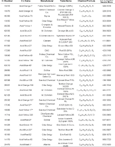
Table 1. Fifty dyes included in the mini-database. ... 39
Table 2. Results of the database search using the Agilent B.04 Qualitative Analysis
software. ... 45
LIST OF FIGURES
Figure 1. Flow diagram for forensic fiber examination. ... 5
Figure 2. HPLC schematic ... 14
Figure 3. Negative ESI schematic. ... 16
Figure 4. Quadrupole Time-of-Flight Mass Spectrometer schematic ... 18
Figure 5. Schematic of an FT-ICR cell. ... 20
Figure 6. Cut-away view of an Orbitrap an example ion trajectory shown in red. ... 21
Figure 7. Single acquisition FTMS spectra of Disperse Yellow 42 dye: a) spectrum acquired on 7 Tesla LTQ-FT-ICR mass spectrometer at AGC 1.00×10⁶ and RPFWHM 100,000 at m/z=400, b) spectrum acquired on LTQ-Orbitrap XL at AGC of 1.00×10⁶ and RPFWHM 60,000 at m/z=400 before manual adjustment, and c) spectrum acquired on the LTQ-Orbitrap XL at AGC of 1.00×10⁶ and RPFWHM 60,000 at m/z=400 after manual adjustment. ... 30
Figure 8. The calculated MMA of the monoisotopic peak for the LTQ-FT-ICR data (a and b) and the LTQ-Orbitrap XL data after manual adjustment (c and d) are plotted against the RPFWHM at m/z = 400. The series in black indicates the averages and the 95% confidence intervals of the measurement (N=30). The data points next to each averaged point are the calculated MMA’s for each individual spectrum acquired. The AGC target values evaluated: a and c) 5.00×10⁵ and b and d) 1.00×10⁶. ... 32
Figure 9. The relative abundance of 34S1 to the monoistopic peak (left hand axis) for the LTQ-FT-ICR data (a and b) and the LTQ-Orbitrap XL data after manual adjustment (c and d) are plotted against the RPFWHM at m/z = 400. The χ2 value for the entire isotopic distribution is also plotted (right hand axis) with the red filled triangles (▲) being the calculated χ2 value. The average sulfur peak abundance (N=30) is the black circle series with 95% confidence interval error bars. The points next to each averaged point are the sulfur peak abundances for each individual spectrum. The gray bar indicates the range of natural variation of the 34S isotope as reported by NIST, 3.976%-4.734% (103). The AGC target values evaluated: a and c) 5.00×10⁵ and b and d) 1.00×10⁶. ... 34
Figure 10. Vacuum filtration set-up for HPLC-MS solvent preparation. ... 41
Figure 11. Dye structures and their corresponding spectra containing for three of the dyes used in the construction of the database with examples of the three chromophore most commonly found in acid dyes; a) C.I. Acid Blue 113 containing two azo groups (shown in red) as well as two sulfonic acid groups resulting in both [M-H]1- and [M-2H]2- in the spectrum, m/z 636.1000 and m/z 317.5468, respectively; b) C.I. Acid Blue 25 containing an anthraquinone chromophore (shown in red) and characteristic spectrum with [M-H]1- at m/z 393.1549; and c) C.I. Acid Green 16 containing a triphenylmethane functional group (shown in red) and characteristic spectrum with a molecular ion of [M-H]1- at m/z 593.1774. ... 44
Figure 12. Results of the k-NN analysis using Matlab® software. All 59 data points describing the 50 dyes are shown with unknown 9 inserted into pattern space, shown in red. The descriptors used for the k-NN analysis were k’, mass, M+1, and M+2 isotopic abundances. ... 48
Figure 14. Unknowns with their respective database matches plotted against the first two priciple components. ... 50
Figure 15. Atlas Ci3000+ Xenon Fade-Ometer used for timed photo-degradation study. ... 54
Figure 16. UV-vis spectra of C.I. Acid Green 16 at time points 0-hours (blue) and 40-hours (green). ... 56
Figure 17. Isotopic distribution for C.I. Acid Green 16 over all time points, except for 40-hours. ... 57
Figure 18. Overlaid MS spectra of C.I. Acid Red 361 at time points 0-hours (purple) and 40-hours (blue) with the dye structure inset. ... 58
Chapter 1. Introduction 1.1Purpose
The effectiveness of fibers, a type of trace evidence, in the courtroom depends on the
certainty to which they can be traced back to its source using their physical and chemical
characteristics. Isolation and identification of fibers are important to the forensic community
because of their ease of transfer to the crime scene and potential to provide meaningful
insight into the location of the crime or event. Fibers are a common type of trace evidence
found at crime scenes with as many as 100-10,000 fibers being transferred by the act of
sitting on a seat (1) and were key evidence in the convictions of Ted Bundy and Wayne
Williams as well as many others (2). In both cases, the ability to identify fibers found on the
victims and match them back to a known source proved invaluable for the prosecution. With
the current emphasis on DNA analysis in forensics, much work is being done to prove that
fibers can still offer valuable insight in the courtroom (3). The purpose of this work is to
start the construction of a Liquid Chromatography-Mass Spectrometry (LC-MS) database of
dyes extracted from textile fibers. The database will provide mass spectra of known dyes to
forensic laboratories for comparison to questioned fibers found at crime scenes.
1.2Research Objective
The objective of this research is to create a comparative LC-MS dyed fiber database
for use in forensic cases. The database would initially consist of automotive fibers from a
variety of vehicles of different makes and models and will eventually branch out to other
1. Comparison of the analysis capability of the LTQ-FT-ICR and the LTQ-Orbitrap
XL in regards to the sulfur [M+2] isotopic peak and the whole isotopic
distribution generated by C.I. Disperse Yellow 42.
2. Development of a fifty acid dye example database consisting of LC-MS data from
raw dye powders. Use of the database to accurately identify ten unknown dyes
(five dyes from the database and five dyes not included in the database) will be
examined.
3. LC-MS analysis of acid dyes extracted from nylon fibers after photo-degradation
to simulate the exposure of fabrics to UV light over time.
The overall objective of this research is to show the advantages that an LC-MS
comparative dye database would contribute to the forensic field when used in conjunction
with current fiber analysis techniques.
Chapter 2. Literature Review 2.1 Acid Dyes
Dyes are classified according to their chemical class (e.g., azo, anthraquinone,
triphenylmethane) or application method. Acid dyes are typically applied to nylon, wool,
and silk fibers under acidic conditions, which generate protonated amines in the fibers, and
establish ionic bonds between the negatively charged, sulfonated dyes and the protonated
fibers (4). There are approximately 2354 acid dyes in the Colour Index that are often used in
combination to give fabrics the desired color and within the acid dye class there are several
found in acid dyes are azo, anthraquinone, and triphenylmethane. Less common systems are
based on pyrazalone, hydrazones, azine, nitrodiphenylamine, and phthalocyanine. Azo dyes
are highly versatile and can be used to produce a large color range while the other dye
chemical classes are more restricted. For example, anthraquinoid derivatives are mostly red
to blue and have high washfastness, while xanthene-based dyes tend to be bright red-pink (4).
Dyes vary significantly in their chemistries helping them to impart a wide range of colors on
many different fiber types.
2.2 Forensic Dye Analysis
Current forensic dyed fiber analysis methods involve various levels of analytical tools
yielding information that is used in combination to maximize the usefulness of the analysis
(5). Identification of the dye found in colored fibers in addition to specific fiber properties
adds another level of discrimination to fiber analysis and the use of mass spectrometry (MS)
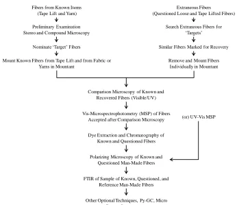
introduces molecular specificity to the analysis. Figure 1(6) shows a flow chart of methods used during forensic fiber analysis. The nature of the fibers, whether natural or man-made,
along with the starting material of the evidence, fiber or fabric etc, determines the
combination and order of the analysis methods utilized. When choosing target fibers, fibers
of interest that will be used as evidence, investigators look for characteristics that will help
increase the discriminatory value of the fiber, for example, the occurrence of the fiber in the
textile industry and the physical characteristics such as coarseness and fluorescence (6).
Common fibers are considered to be less useful; however, a common fiber type, such as a
All aspects must be considered when choosing the optimal target fibers to associate a suspect
with a crime.
Microscopy (7-12), infrared spectroscopy (IR) (13-25), thin-layer chromatography
(TLC) (26-36), and UV-visible microspectrophotometry (MSP) (32, 35, 37-40) have all been
researched extensively for their application to forensic fiber analysis and are typically used in
investigations. Raman spectroscopy (25, 41-49) has also been investigated for potential use
in forensic fiber analysis but has not yet been utilized in a majority of forensic laboratories
for fiber analysis purpose. The development of automated extraction and analysis techniques
is an attractive possibility for use in the field during evidence collection. The automation of
extraction of dyes from fibers (50) for analysis by capillary electrophoresis (CE) (50-56) has
been studied by Morgan and coworkers in hopes that a suitable method will be developed for
forensic use. HPLC (57-63) and MS (54, 55, 60-68) analysis methods have also been
Figure 1. Flow diagram for forensic fiber examination.
The forensics field has been heavily focused on DNA analysis because of its high
discriminating capability which has prompted labs to investigate the individuality of fibers
and their significance as evidence (1, 8, 40, 69-80). Biermann and coworkers studied
diameter, cross section, fluorescence, delustrant particle size, birefringence, and the UV-Vis
spectra of 255 blue polyester samples and found 3 random matches (1). In theory, the
addition of LC-MS to the analysis protocol would reduce this number to zero random
matches making it an invaluable tool for forensic analysis where a high level of
discrimination is important.
Fibers from Known Items (Tape Lift and Yarn)
Extraneous Fibers (Questioned Loose and Tape Lifted Fibers)
Preliminary Examination Stereo and Compound Microscopy
Nominate ‘Target’ Fibers
Mount Known Fibers from Tape Lift and from Fabric or Yarns in Mountant
Search Extraneous Fibers for ‘Targets’
Similar Fibers Marked for Recovery
Remove and Mount Fibers Individually in Mountant
Comparison Microscopy of Known and Recovered Fibers (Visible/UV)
Vis-Microspectrophotometry (MSP) of Fibers Accepted after Comparison Microscopy
Dye Extraction and Chromatography of Known and Questioned Fibers
Polarizing Microscopy of Known and Questioned Man-Made Fibers
FTIR of Sample of Known, Questioned, and Reference Man-Made Fibers
Other Optional Techniques, Py-GC, Micro Raman Spectroscopy
The current required analytical tests for fiber evidence are outlined in the Forensic
Fiber Examination Guidelines put together by the Scientific Working Group on Materials
Analysis (SWGMAT). A combination of methods in an order that maximizes accuracy,
precision, and production is required. There are two purposes to forensic fiber analysis;
identification of questioned fibers and comparison of questioned fibers to known fibers (81).
The purpose of the analysis helps to determine the methods and techniques employed for the
analysis.
2.2.1 Microscopy
Stereomicroscopy, comparison microscopy, PLM, fluorescence microscopy, and
MSP methods are commonly employed for analysis of dyed fibers. Each microscope is used
to determine a different property of the fiber to be used to get the highest discrimination
capability possible for the identification and comparison of questioned samples.
Stereomicroscopy is a lower magnification technique but allows for large sample
sizes typically encountered during the fiber recovery process from tape and large pieces of
evidence (6). Once the target fibers are recovered using the stereomicroscope with both
reflected and transmitted light, other analytical methods are employed to study the fiber.
Comparison microscopy is used in forensic fiber examination for side by side
comparison of known and questioned fibers for points of similarity and points of difference
(6). A comparison microscope consists of two compound microscopes connected by an
optical bridge. They can also be fitted with addition elements, such as a polarizing light
Microscopy is used to view the physical properties of the fiber that are present from
manufacturing as well as from use. Man-made fibers are typically smooth and uniform;
however, wear patterns and signs of age can provide valuable insight into the fiber history.
Some physical characteristics that can be determined are diameter, cross-sectional shape,
surface features, fluorescence (using fluorescence microscopy), internal detail, and color.
PLM is used to determine the optical properties of questioned fibers; which in most
cases are sufficient to determine fiber type. Optical properties come from the chemical
composition of the fibers or changes in orientation and spacing of constituents that occur
during spinning and treatment of the fibers (81). PLM is used to determine properties such
as sign of elongation, quantitative birefringence, isotropic refractive index (niso), and the
refractive index for light vibrating in a plane parallel to the fiber (n║) or in a plane
perpendicular to the fiber (n┴) (81).
2.2.2 UV-visible Microspectrophotometry (MSP)
In forensics, UV-visible MSP is a quick non-destructive method to analyze small
colored fibers for comparison purposes by recording the UV-visible spectrum without having
to remove the fiber from the microscope slide. UV-visible spectroscopy is used to study
conjugated systems making it an ideal method for dye analysis because of the extended
conjugation systems in dye molecules needed to produce color. It is used for the study of
metemeric fibers; fibers that appear to be the same color but were created using different
dyes. MSP is a single beam instrument but is able to store incident light intensity to use for
a double beam instrument (81). Grieve and coworkers investigated the percentage of
matching spectra of blue, red, and black dyed cotton and found that within the red and black
color classes less than 1.5% of spectra matched and only 0.2% of the blue spectra matched
(32). Macrae and coworkers also investigated the discrimination capability of MSP but
focused on wool fibers. In their comparison of blue wool fibers, they found that comparison
microscopy with white light only offered a discrimination of 47% but the discrimination
capability of MSP was 99%, the same as their findings for TLC (37); however, MSP is
nondesctructive and can be used on fibers with low dye concentrations when extraction and
analysis via TLC is not possible.
2.2.3 Infrared (IR) and Raman Spectroscopy
IR is used for the identification of the fiber polymer through investigation of the
vibrational frequencies of the molecules after irradiation in the IR region. FT-IR has
increased the speed and sensitivity of IR spectroscopy making it a useful and often employed
tool in forensic science. FTIR databases have been developed for simple polymer
identification in the forensics lab (13, 15). Grieve and coworkers studied FTIR spectra of
dyed acrylic fibers and were able to determine absorptions of the dyes along with the
characteristic polymer absorptions (21).
Resonance Raman works by using a laser excitation in resonance with the dye
molecule to cause molecular vibrations. It is an attractive tool for forensic dyed fiber
analysis because it is more sensitive and specific than IR spectroscopy and can also detect
used for the in-situ detection of reactive dyes at picrogram concentrations on cotton after
digestion for 21 hours (41, 44). Raman microprobe spectroscopy was successfully utilized for
fiber polymer characterization without sample preparation; however, the dye needed to be
extracted to obtain spectra for both the dye and the polymer (43). Resonance Raman has
been successfully employed for the detection and discrimination black dyes of different
textile types (46, 48) and of reactive dyes on cotton (42). Raman spectroscopy has potential
for investigation of dyed fibers for forensic purposes; however, much research and
standardization of methods need to be done.
2.2.4 Thin Layer Chromatography
TLC offers the advantages of convenience, the ability to separate multiple samples on
the same plate, and easy detection through the addition of colored reagents. In TLC the
samples are spotted on a plate coated with an adsorbent material that acts as the stationary
phase, usually silica gel, and placed vertically in a chamber with a solvent or solvent mixture,
depending on the chemical nature of the dye being studied, which acts as the mobile phase.
The mobile phase travels up the TLC plate via capillary action and the analytes of the sample
undergo separation based on their different migration rates due to interactions with the
stationary phase and the mobile phase. The distance the spot travels from its starting position
divided by the total distance the mobile phase traveled gives the capacity factor (k’) that can
be used for compound identification (82). The k’ of known and questioned samples can be
TLC is used in forensic science for the analysis of dyes extracted from forensic fiber
evidence when comparison microscopy and microspectrophotometry of the visible range are
not able to discriminate between fibers of interest (83). TLC cannot be used for forensic use
in the case of sample limited evidence and can only be used for comparisons to a known
fiber. Beattie and coworkers developed methods for the extraction and TLC analysis of acid,
disperse, and basic dyes from nylon, polyester, and polyacrylonitrile fibers finding them
useful only in a comparison capacity in the forensic field (26, 29). TLC was used to compare
historic Grübler dyes to their modern day counterparts to ensure correct labeling and purity
for future manufacturing purposes (36). Their findings highlight the issue of continuity
between different dye manufacturers across the globe which could introduce problems in the
development of a dye database if there are dyes that are mislabeled or have excessive
impurities.
2.2.5 Pyrolysis-Gas Chromatography
Pyrolysis involves the thermal decomposition of analytes into molecular fragments
characteristic of the initial fiber. Pyrolysis can be used in conjunction with GC and a variety
of detectors depending on the desired information. Detectors used with Py-GC include flame
ionization (FID), alkali flame ionization (AFID), flame photometric (FPD), electron capture
(ECD), and MS (6). The detectors provide retention times of characteristic components that
can be identified using databases or known fiber samples. MS detectors offer higher
sensitivity and provide the most information out of the detectors mentioned because they
2.2.6 High Performance Chromatography and Capillary Electrophoresis
HPLC methods have been developed and successfully utilized for the analysis of dyes
on textile fibers for forensic use. HPLC is a quantifiable method that also could be utilized
for the construction of databases making it advantageous over TLC. Methods have been
developed for the analysis of acid (57), basic (58), and disperse dyes; however, analysis of
acid dyes typically involves the use of ion pairing agents rendering it useless for MS
detection. Mottaleb and coworkers attempted HPLC-FTIR with a thermospray interface for
dye analysis to produce FTIR chromatograms and IR spectra but found the technique lacked
sensitivity (59). HPLC and CE separation conditions vary based on the chemical
composition of the analytes of interest. Different experimental conditions have been
developed for each dye type for both HPLC; however, standardized conditions have still not
been established.
CE separates small volumes of ionic species in a capillary filled with buffer solution
with an applied high voltage filled, based on their charge to mass ratio. When utilized with
MS detection the capillary effluent goes directly into the electrospray interface (82). CE-MS
with negative ion electrospray ionization has been successfully used to identify anionic
metalized azo and formazan dyes (51). Morgan and coworkers have developed automated
extraction methods with different solvent conditions suitable for each dye type for analysis
via CE. Diode- array detection (DAD) was used for the dye types (50, 56); however, when
investigating small sample size DAD was not deemed useful, instead MS detection coupled
with CE was used for sample sizes as small as 2 mm fibers (55) and was also successful in
2.2.7 Mass Spectrometry
MS is a powerful potential tool for forensic analysis of dyes extracted from textiles
because of its high sensitivity and reproducibility as well as the molecular level of
information it provides. There has also been discussion of the usefulness of an MS dye
database for forensic purposes (60, 61). Many research groups have been successful at the
HPLC-MS analysis of fiber dyes. Tuinman and coworkers analyzed acid dyes extracted from
nylon via MS using direct infusion methods for comparison of dyes while also utilizing
MS/MS for dyes of the same m/z (65). HPLC of acid dyes has been difficult and typically
requires mobile phase additives that are not compatible with MS because they cause signal
suppression. HPLC-MS analysis has been achieved through removal of the additives before
injection into the MS (63) while some groups have reported the use of triethylammonium
acetate to be successful in small quantities (60). MALDI –MS has also been considered for
dye analysis because of its easy sample prep and ability to be used with dyes that are
insoluble (66, 68). While there is still work to be done in the development of the analysis of
dyes by MS, there is much potential for the development of a database that could be utilized
across forensic laboratories.
2.3 Instrumentation
2.3.1 High-Performance Liquid Chromatography
Liquid chromatography (LC) began in the 1905 with classical column
chromatography separation of colored pigments by Michael Tswet (84). In column
collected as they elute from the end of the column. Traditional column chromatography is
time consuming and requires a new column be used for every sample (84). Paper
chromatography was invented in 1943 by A.J.P. Martin and the addition of a thin layer of
silica over the chromatography paper or glass plate led to the development of thin-layer
chromatography (TLC) (84). The next stage of the development of LC was realized when
the first high-performance liquid chromatography (HPLC) paper appeared in 1966 and by
1971 the first HPLC book was published (84).
HPLC is a separation technique that involves a liquid mobile phase and a stationary
phase. The mobile phase can be manipulated easily to accommodate a variety of chemical
compositions. Samples need not be volatile to undergo HPLC separation, allowing a wider
range of compounds to be analyzed than with GC (84). In reverse phase HPLC, the sample
is injected via an autosampler into a column along with a constant flow of solvent. A pump
keeps the solvent flow rate constant while the analytes of interest partition between the
mobile phase and stationary phase undergoing separation. The detector plots out the results
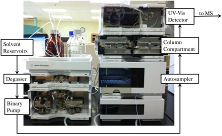
Figure 2. HPLC schematic
Mass transport occurs by way of two mechanisms through the column; mobile phase
flow and molecular diffusion. The mobile phase flow carries solutes through the column
while individual analyte molecules diffuse in and out of the stationary phase. All analytes
spend the same amount of time in the mobile phase; therefore, separation occurs through the
differences in the amount of time the analytes spend in the stationary phase (84). The
stationary phase is chosen based on the compounds being separated. The two main forms of
HPLC are Reverse Phase HPLC (RPLC) and Normal Phase HPLC (NPLC). This review will
focus on RPLC.
Reverse phase liquid chromatography (RPLC) is used for separation of moderately
polar to nonpolar compounds. In RPLC, the mobile phase is more polar than the stationary
Solvent Reservoirs
Degasser
Binary Pump
Column Compartment
UV-Vis Detector
Autosampler
phase and compounds are eluted from the column in order of decreasing polarity (84).
Coupling of HPLC to MS for acid dye analysis has been difficult due to the need for
ion-pairing reagents that are not volatile and therefore not compatible with MS detection (63).
The use of volatile amines has proven successful when used in small concentrations (< 2.5
mM) to detect aromatic sulfonates in wastewater (85) and in the identification of dyes
extracted from fibers (60).
2.3.2 Electrospray Ionization
The coupling of HPLC and MS was initially a problem before the development of
electrospray ionization (ESI) due to the use of a liquid mobile phase and the involatility of
analytes. ESI is a soft ionization method that utilizes a charged capillary to send solvent
droplets into an atmospheric pressure region towards a counter electrode (86). As the
droplets pass through the atmospheric pressure region, they are desolvated by nitrogen drying
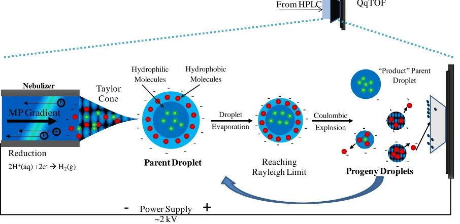
gas before entering a high vacuum region and travelling into the mass spectrometer, Figure 3. There are four steps that occur during the ESI process; droplets of HPLC mobile phase and analyte are formed then become charged, followed by desolvation and the formation
analyte ions (87). There are two main theories about the chemistry taking place during this
Figure 3. Negative ESI schematic.
The charge residue model proposes the existence of an ultimate droplet that contains
only one species. The solvent evaporates and the surface energy of the droplet decreases
until the Rayleigh limit is reached and the drops undergo repeated Coulombic fissions until
only the “ultimate droplet”, consisting of a gas phase analyte molecule and charge originating
from surface charge of the evaporated droplet, remains (88). The ion evaporation model
theorizes that as the solvent evaporates, the charges cause electrostatic repulsion and product
droplets are formed. The product droplets continue to undergo evaporation until the
Rayleigh limit is reached and smaller droplets containing a few molecules and a single
charge are ejected and travel to the MS (89). Both models have been researched extensively
finding that the ion evaporation model is ideal for the explanation of small molecules but the
charge residue model is more plausible for macroions such as proteins (90).
QqTOF
MP Gradient
Reduction
2.3.3 Quadrupole-Time-of-Flight
Q-TOF is a triple quadrupole mass spectrometer with the third quadrupole replaced
by a time-of-flight (TOF) mass analyzer. The first quadrupole is mass resolving followed by
an r.f. only hexapole collision cell that leads into a TOF mass analyzer. When used in single
MS mode the first two quadrupoles act as ion focusing and the ions are detected in the TOF.
TOF is a kinetic energy dependent mass analyzer that offers the advantages of high
sensitivity, high mass resolution, and high mass accuracy. Flight times are measured in
microseconds with nanosecond differences between ions of the closest m/z. In single MS,
mode the TOF offers 2 ppm mass accuracy and femtomole to attomole limits of detection.
The ability to multiply charge the ions allows the instrument to have an unlimited mass
range(86).
Equation 1. Relationship between flight time and m/z.
In TOF, flight times are proportional to m/z, Equation 1(86), where t is ion flight time, m is mass, z is charge state of the ion, e is electron charge, and Uex is the extraction
voltage. The reflectron was added to overcome any kinetic energy differences that would
alter the time of flight to m/z proportionality. The reflectron is a set of lenses with a voltage
gradient that acts as an ion mirror, at the end of the flight tube used to help diminish the
them back out with the same speed with which they entered; however, the ions with greater
kinetic energies penetrate farther into the field causing them to have a longer flight path than
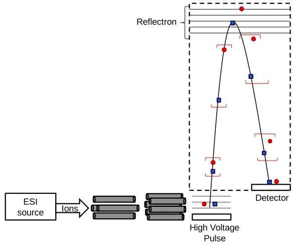
the ions with less kinetic energy(86). In Figure 4, the flight paths of two ions of the same
m/z are shown. The ion depicted by the circle leaves the pulse plate with a higher kinetic
energy than the ion depicted by the square. Both ions travel the flight tube and enter the
reflectron; however, ion with the higher kinetic energy penetrates farther into the reflectron
before it changes directions and is ejected at the same speed at which it entered enabling it to
catch up with the ion of lower initial kinetic energy at the detector and allowing both ions to
be detected at the same time.
Figure 4. Quadrupole Time-of-Flight Mass Spectrometer schematic
The TOF is equipped with orthogonal acceleration, which enables it to be used with
the ESI ion source. Without orthogonal acceleration the TOF would not be compatible with
ESI
source Ions
Reflectron
Detector
a continuous ion source such as ESI due to the spatial and energy spreads of the ions
resulting from the continuous flow ion source (91).
2.3.4 Fourier Transform- Ion Cyclotron Resonance Mass Spectrometry
Fourier transform- ion cyclotron resonance (FR-ICR) is a high resolving power mass
spectrometry technique utilizing a uniform magnetic field. Gas-phase ions in the presence of
a uniform magnetic field will follow a circular path perpendicular to the direction of the
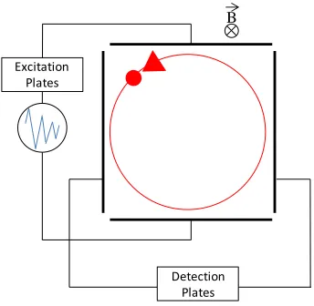
magnetic field at a frequency related to their m/z (86). Two excitation plates, positioned
opposite one another, Figure 5, irradiate the ions in the ICR cell with a uniform rf only electric field (excitation pulse) at the same frequency as their natural resonance, increasing
their orbit and causing phase coherence of ions of the same m/z. Two opposite parallel
detection plates measure an image current (time-domain signal) that is Fourier transformed
into a frequency domain signal, that is converted to mass domain by Equation 2, where ωc is
cyclotron frequency, q is charge, Bo is magnetic field, and m is mass (92).
Equation 2. Relation of cyclotron frequency to mass (m) and charge (q) in a uniform magnetic field (B)
Figure 5. Schematic of an FT-ICR cell.
2.3.5 Orbitrap Mass Spectrometry
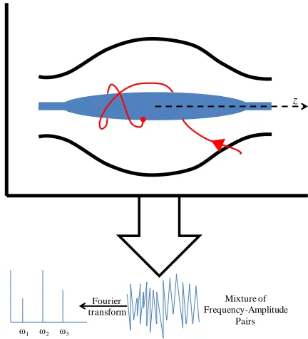
The Orbitrap is considered a modified Knight-style Kingdon trap that consists of two
coaxial axisymmetric electrodes and an outer barrel shaped surface and an inner spindle
shape electrode (93, 94), Figure 6. Detection in the Orbitrap is similar to that in FT-ICR; however, it does not use a magnetic field and the ions do not undergo excitation. The ions
are electrostatically trapped in the Orbitrap while rotating around the central spindle
electrode and oscillating axially. The image current generated by the ions is Fourier
transformed to get the axial frequency, which can be converted to m/z via Equation 3(95).
Equation 3. Relationship between m/z and axial frequency.
Excitation
Plates
B
Figure 6. Cut-away view of an Orbitrap an example ion trajectory shown in red.
2.4 Spectral Accuracy and Sulfur Counting
High resolving power (RP) mass spectrometers have the ability to provide high mass
measurement accuracy (MMA) which is invaluable in defining the elemental composition of
unknowns (93, 96, 97). However, MMA only takes into account the monoisotopic peak, not
the entire isotopic distribution. High RP instruments produce spectra that contain useful
isotopic information that can be utilized to provide more confident elemental compositions.
Isotopic distributions contain several peaks whose relative heights are due to natural isotopic
abundances and can be used to aid in the elemental composition determination of an
unknown substance (98). For example, the relative abundance of the A+1 peak compared to
the monoisotopic peak in conjunction with the natural abundance of the 13C isotope is
indicative of the total number of carbons in the compound (86). The relative abundance of
z
Mixture of Frequency-Amplitude
Pairs Fourier
transform
the A+2 peak in the distribution can be used to accurately predict the presence and the
number of atoms with A+2 isotopes, such as sulfur, bromine, and chlorine (98, 99).
Spectral accuracy is the ability of the mass spectrometer to correctly measure the
isotopic distribution of ions (100). Accurate isotopic ratios are necessary to increase
confidence in elemental composition assignments. Isotopic distribution evaluation analyses
have been reported in the literature using Orbitrap (101) and FT-ICR spectra (102) as a way
to reduce the number of possible elemental composition assignments for a given species.
Junot et al. found that absolute ion abundance was the main factor affecting the isotopic
distribution and mass accuracy while studying isotopic distributions in the LTQ-Orbitrap
(101). They also found that liquid chromatography improved the relative isotopic
abundances of the distribution, which is attributed to decreasing the number of isotopic
distributions present (101). Stoll et al. evaluated different methods, such as calculated
double-bond equivalence, ion state, and isotopic distribution simulation and comparison, to
compare theoretical and experimental data as a means of narrowing elemental composition
assignments (102). In the 25 compounds studied, they found that isotopic distribution
evaluation led to a decrease in the number of possible elemental composition assignments for
a given species by an average of 90.6% (102). Thus, the accurate measurement of not only
the mass (MMA), but also the isotopic distribution can be significantly exploited for the
confident identification of elemental compositions in high RP mass analysis.
Using high RP MS, it is also possible to count (in some cases estimate) the number of
specific atoms (C, S, Br, Cl, etc.) in a compound through analysis of the A+1 and A+2
height of the resolved doublet at the A+2 peak, the number of sulfurs in a molecule can be
determined. The natural abundance of the 34S isotope is 3.976%-4.734%, as reported by
NIST (103). When sulfur is present in a compound, high RP MS (≥30,000) is capable of
resolving the A+2 peak into a doublet with a mass difference of 0.0109 Da between the
peaks. The lighter peak, indicative of the 34S1 isotope, has a mass difference of 1.9958 Da
from the monoisotopic mass and the heavier peak, indicative of the 13C2 isotopic peak, has a
mass difference of 2.0067 Da from the monoisotopic mass(99). The relative abundance of
the 34S peak in comparison to the monoisotopic peak depends on the number of sulfur atoms present in the compound. For each sulfur present in the compound, the relative abundance of
the 34S peak increases by the natural abundance of the 34S isotope. The ability of high RP mass spectrometers to count sulfurs has been studied previously (104-106). Marshall and
coworkers used sulfur-counting as a means to characterize the p16 tumor suppressor protein
(104), and also later in the study of glycosphingolipids (106). Hoye and coworkers applied
sulfur-counting to the study of sea lamprey pheromones (105).
Automatic gain control (AGC) target is a means of controlling the ion population
during analysis (107, 108). Higher ion populations increase space charge effects and can
lead to decreased MMA; additionally, variable ion populations can allow for variable MMA
and spectral accuracy for each individual scan. Thus, AGC allows one to keep the total ion
population ‘constant’ which significantly decreases the analytical variability of the
2.5 Forensic Chemometric Applications
The application of chemometrics has been studied extensively for forensic use.
Principal component analysis (PCA) is a statistical method that analyzes variables of multiple
samples and reduces them to principle components that can be graphed and analyzed to
determine which principle components have the most impact on the data. The number of
principal components is equal to the number of descriptors in the data set. The samples are
plotted out on the principal components that encompass the greatest amount of variance in
the data set (110). PCA can be used in conjunction with cluster analysis and classification
algorithms to identify unknowns by mapping their distance in pattern space to known objects.
PCA and cluster analysis were used on Raman data of forensic paint samples (111), and
narcotics (112). PCA and k-NN were used together to effectively identify heroin batches
(113). PCA and K-means have been used in conjunction for the successful evaluation of ball
point pen inks analyzed via UV-Vis (114), and HPLC (115), as well as for forensic soil
analysis (114).
The analysis of ballpoint pen inks using HPLC and UV-Visible spectroscopy has be
successfully used to classify pen type (115). In the analysis of red, black, and blue pens they
were most successful with an 87.5% classification of the blue ballpoint pen by using class
distances found after PCA analysis; however the addition of LC-MS data to these analyses
would increase the correct classification of the pens due to the addition of molecular
information (115). PCA and K means cluster analysis were used for the successful
identification of 100% of the blue ball-point pen inks studied based on their visible spectra
framework for the development of a database for the identification of dyes found in
questioned fibers.
Chapter 3. Spectral Accuracy and Sulfur Counting Capabilities of the LTQ-FT-ICR and the LTQ-Orbitrap XL for Small Molecule Analysis
In Chapter 3, the capabilities of the LTQ-FT-ICR and the LTQ-Orbitrap XL for
determination of elemental composition through utilization of MMA, spectral accuracy, and
sulfur counting are compared. AGC target and resolving power were varied in both the
LTQ-Orbitrap XL and the LTQ-FT-ICR as a means of understanding the capabilities and
limitations of the instrumentation pertaining to small molecule analysis. Furthermore, the
authors present two separate data sets acquired on the LTQ-Orbitrap XL. The initial data set
taken on the LTQ-Orbitrap XL produced spectra with MMA > 2.5 ppm and inaccurate sulfur
counting analyses despite the instrument passing all user tuning procedures and being
calibrated per the manufacturer specifications. Thus, detailed inspection and manual tuning
of the installation parameters by the manufacturer followed, and sub-ppm MMA was
achieved in subsequent data acquisition (vide infra).
3.1Experimental
3.1.1 Disperse Yellow 42 Sample Preparation
Color Index (C.I.) Disperse Yellow 42, C18H15N3O4S, (DY 42), trade name Foron
Yellow AS-FL, was obtained from Clariant (Batch CHAA109775) for analysis. To purify
brought to a boil while stirring on a hot plate. The sample was filtered hot, and the filtrate
was evaporated to dryness. The dried sample was collected for analysis.
Two stock solutions (1 mg/mL) of the purified dye powder were prepared in 50:50
acetonitrile:water. The samples were diluted to 10 µg/mL for analysis on a hybrid linear ion
trap, Orbitrap mass spectrometer, LTQ-Orbitrap XL (Thermo Scientific, San Jose, CA) and
a hybrid linear ion trap, Fourier transform ion cyclotron resonance mass spectrometer,
LTQ-FT-ICR, (Thermo Scientific, San Jose, CA) with a 7 Tesla superconducting magnet.
3.1.2 LTQ- FT-ICR Analysis
The instrument was calibrated per the manufacturer specifications. The 10 µg/mL
sample was introduced by direct injection via an in-house nanoESI source. The following
instrument parameters were used for all analyses on the LTQ-FT-ICR: capillary voltage and
temperature of 42 V and 225°C, respectively, and a tube lens voltage of 120 V. Thirty full
range mass spectra (150-2000 m/z) were collected at two AGC targets: 5.00×10⁵ and
1.00×10⁶. The full-width-half-maximum resolving powers (RPFWHM at m/z=400) evaluated
were 12,500, 25,000, 50,000, 100,000, and 200,000.
3.1.3 LTQ-Orbitrap XL Analysis
The instrument was calibrated per the manufacturer specifications with the lock-mass
feature enabled. All instrument parameters were the same as specified for the LTQ-FT-ICR
m/z) spectra were collected at each set of conditions. The following RPFWHM at m/z=400
were used during the LTQ-Orbitrap XL analysis: 7,500, 15,000, 30,000, 60,000, and 100,000
at m/z=400. The same AGC targets were used as with the LTQ-FT analysis.
3.1.4 Data Analysis
The MMA, χ2 value for the isotopic distribution, and relative abundance of the A+2 sulfur peak were calculated. Equation 4 is the formula used to calculate the MMA of the monoisotopic peak at each resolving power and AGC target.
Equation 4. MMA formula
The χ2 value for the relative abundances in relation to the monoisotopic peak in the
isotopic distribution of DY 42 was calculated to quantify spectral accuracy; shown as
Equation 5 (116). The χ2 value was calculated for each spectrum at each resolving power and AGC target studied.
Equation 5. χ2 formula
The number of sulfurs was found by determining the relative abundance of the sulfur
peak compared to the monoisotopic peak and multiplying by the 32S:34S natural composition
ratio where A+2 and A are the experimenetal peak intensities of the 34S and monoisotopic peak, respectively. 32STheoretical and 34STheoretical are the natural isotopic compositions as
reported by NIST of the 32S and 34S, respectively.
Equation 6. Formula used to calculate the number of sulfurs in the compound using the isotopic peak height.
3.2 Results and Discussion
Two data sets will be discussed for the LTQ-Orbitrap XL in comparison to a data set
produced by the LTQ-FT-ICR. The initial data set for the LTQ-Orbitrap XL produced
results that are not consistent with the potential specifications reported for an Orbitrap
instrument by the manufacturer (e.g. sub-ppm MMA). Additionally, despite passing all user
tuning methods and being calibrated per the manufacturer specifications, this group has
observed sub-par MMA for this instrument since installation. Furthermore, before the
installation parameters were adjusted, sulfur counting experiments in the LTQ-Orbitrap XL
did not produce the correct number of sulfurs for a standard molecule. Thus, in a personal
communication with Alexander Makarov (117), he immediately concluded that the Orbitrap
was not performing optimally upon assessment of the data. During his assessment, he
parameters are not included in the user tune method, and it is not recommended that these
parameters be changed by anyone other than a manufacturer engineer. The parameters that
were changed include deflector voltage on the Orbitrap and the injection level of the central
electrode along with minor adjustments to the lens voltages and pulse voltages on the C-trap.
Upon manual optimization of these installation parameters, the second set of data from the
LTQ-Orbitrap XL was collected, which produced significantly higher quality data with
respect to MMA and spectral accuracy.
Figure 7a, Figure 7b, and Figure 7c are example spectra of each data set for DY 42 produced by LTQ-FT-ICR, LTQ-Orbitrap XL (before manual adjustment of the installation
parameters), and LTQ-Orbitrap XL (after manual adjustment of the installation parameters),
respectively. The LTQ-FT-ICR spectra were taken at a RPFWHM at m/z=400 of 100,000 and
an AGC target of 1.00×10⁶. Both the LTQ-Orbitrap XL spectra in Figure 7b and Figure 7c
(before and after manual adjustment of the installation parameters, respectively) were
acquired at an RPFWHM at m/z=400 of 60,000 and an AGC target of 1.00×10⁶. The red dots
above each peak in all three spectra are indicative of the theoretical peak heights for the
isotopic distribution of DY 42. Figure 7b and Figure 7c display the vast difference in the results acquired before and after manual adjustment of the installation parameters. The
MMA is an order of magnitude better, and the spectral accuracy is significantly better (lower
2
value – vide infra) upon parameter adjustment of the installation parameters. These data
suggest that a standard molecule or procedure must be used (in addition to the tuning
protocol provided by the manufacturer) to determine whether or not the instrument is
installation parameters, Figure 7a (LTQ-FT-ICR) and Figure 7c (LTQ-Orbitrap XL) show that the two instrument platforms are both capable of acquiring the correct results.
3.2.1 Mass Measurement Accuracy
Plots of the MMA of the monoisotopic peak of each spectrum and the average MMA
with 95% confidence intervals at each resolving power are shown for the LTQ-FT-ICR and
LTQ-Orbitrap XL (after installation parameter adjustment) in Figure 8. Figure 8a and Figure 8c are shown at an AGC target of 5.00×10⁵ and Figure 8b and Figure 8d are shown at an AGC target of 1.00×10⁶. The oleamide ion (m/z 282.2791) was used for lock-mass during the LTQ-Orbitrap XL analysis. Lock-mass is an internal m/z standard used to correct
for fluctuations due to temperature and high voltages (96, 118) and can allow for sub-ppm
MMA.
Spectra acquired on the LTQ-FT-ICR produced MMA below 2 ppm for AGC targets
5.00×10⁵ and 1.00×10⁶. The average MMA ± 95% confidence interval of 30 spectra produced by the LTQ-FT-ICR at AGC target 1.00×10⁶ and RPFWHM 100,000 was -1.3 ± 0.1
ppm (Figure 8a). The average MMA ± 95% confidence interval of 30 spectra produced on
the LTQ-Orbitrap XL, before adjustment of the installation parameters, at AGC target
1.00×10⁶ and RPFWHM 60,000 was 2.7 ± 0.2 ppm (Figure 8b). After the installation
parameter optimization on the LTQ-Orbitrap XL, the average MMA ± 95% confidence
interval of 30 spectra at AGC target 1.00×10⁶ and RPFWHM 60,000 was -70 ± 20 ppb (Figure
7c). Upon correction of the LTQ-Orbitrap XL, both instruments performed within manufacturers specifications; however, with lock-mass enabled the LTQ-Orbitrap XL is
capable of ppb mass accuracy. A consistent positive bias and MMA values routinely greater
than 2.5 ppm were observed in the LTQ-Orbitrap XL data before parameter optimization
parameters mentioned above were adjusted on the LTQ-Orbitrap XL, the data quality
improved significantly with MMA values routinely less than 1 ppm.
3.2.2 Spectral Accuracy and Sulfur Counting
The χ2 value of the isotopic distribution was used to “quantify” spectral accuracy in
these experiments; a high χ2 value is indicative of poor spectral accuracy. The calculated χ2 values as a function of resolving power can be seen in Figure 9 at AGC targets of 5.00×10⁵ (Figure 9a and Figure 9c) and 1.00×10⁶ (Figure 9b and Figure 9d), for both the LTQ-FT-ICR (Figure 9a and Figure 9b) and the LTQ-Orbitrap XL (Figure 9c and Figure 9d) . The sulfur peak relative abundance can be seen on the left y-axis of the same plots. Spectral
accuracy plots for initial data produced by the LTQ-Orbitrap XL before manual adjustment
(data not shown) suggest a decrease in spectral accuracy as the resolving power increased,
agreeing with the findings of Erve et al. (100); however, this correlation was not observed
after the instrument parameters were changed on the Orbitrap or in any of the data collected
on the LTQ-FT-ICR. After optimization of the mentioned installation parameters, spectral
Figure 9. The relative abundance of 34S1 to the monoistopic peak (left hand axis) for the LTQ-FT-ICR data (a and b) and the LTQ-Orbitrap XL data after manual adjustment (c and d) are plotted against the RPFWHM at m/z = 400. The χ2 value for the entire isotopic distribution is also plotted (right hand axis) with the red filled triangles (▲) being the calculated χ2 value. The average sulfur peak abundance (N=30) is the black circle series with 95% confidence interval error bars. The points next to each averaged point are the sulfur peak abundances for each individual spectrum. The gray bar indicates the range of natural variation of the 34S isotope as reported by NIST, 3.976%-4.734% (103). The AGC target values evaluated: a and c) 5.00×10⁵ and b and d) 1.00×10⁶.
Erve et al. noted that spectral accuracy decreased as resolving power increased; they
attributed this to isotopic beating (100, 119, 120). However, the closer two frequencies are
the longer the beat period, meaning the specific isotopes interact less during the measurement
to the fact the compounds they studied had a significantly higher m/z (lower frequency) than
this study. In this study, we were able to resolve the 13C2 from the 34S1 isotopic peaks and
thus, determine their individual frequencies in both the LTQ-FT-ICR and the LTQ Orbitrap
XL using the diagnostic mode. The isotopic beat periods for this doublet were 0.116 and
0.196 seconds in the LTQ-FT-ICR and LTQ-Orbitrap XL, respectively, which is small
relative to the measurement period (~1 second) for a typical analysis. In contrast the beat
period for the monoisotopic peak and the A+1 peak in the LTQ-FT-ICR and LTQ-Orbitrap
XL were ~0.0013 and ~0.002 seconds, respectively. While the beat period is much longer
for the A+2 doublets relative to the 13C isotopes (a factor of ~90 for the LTQ-FT-ICR and
149 for the LTQ-Orbitrap) this should be sufficient to provide high spectral accuracy for the
entire isotopic distribution. This is consistent with our findings. Thus, we attribute the
findings of Erve (100), consistent with our LTQ-Orbitrap findings before manual
optimization, to be their instrument settings rather than being related to isotopic beat patterns.
We are currently pursuing these incongruent observations with more detailed studies.
The sulfur peak relative abundances produced by the LTQ-FT-ICR were within the
expected natural abundance range for one sulfur atom at all resolving powers studied for
AGC targets 5.00×10⁵ and 1.00×10⁶, demonstrating the capability of the LTQ-FT-ICR to
accurately resolve the 34S1 and 13C2 peaks and quantify the number of sulfurs.
Analysis of the A+2 peak of the spectrum for the LTQ-Orbitrap XL data acquired
before manual adjustment showed peak heights (≤3% relative abundance) systematically
lower than the theoretical abundance which did not give an accurate indication of the number
data taken after the LTQ- installation parameters were changed are within the expected peak
height range for a compound containing one sulfur. The average sulfur peak height ± 95%
confidence interval for the LTQ-Orbitrap XL at AGC target 1.00×10⁶ and RPFWHM 60,000
before the parameter optimization was 1.82 ± 0.11, compared to 3.91 ± 0.21 after parameter
optimization.
3.3 Conclusions
The small molecule analysis capabilities in the context of MMA, spectral accuracy,
and sulfur counting were compared for the LTQ-FT-ICR and the LTQ-Orbitrap XL. Both
instruments were reported by Thermo Fisher Scientific to be performing at manufacturer
specifications, but initially the LTQ-Orbitrap XL was far outperformed by the LTQ-FT-ICR.
A more in depth inspection of the Orbitrap XL installation parameters, outside of the user
tuning procedure, yielded significantly improved data. Sulfur counting was successful using
the LTQ-FT-ICR and LTQ-Orbitrap XL platforms at AGC targets 5.00×10⁵ and 1.00×10⁶.
Based on these results, the LTQ-Orbitrap XL is a suitable replacement technology for the
LTQ-FT-ICR for small molecule sulfur counting and isotopic distribution analysis to yield
more confident elemental composition assignments.
Due to the LTQ-Orbitrap XL passing all manufacturer tuning procedures, yet still
acquiring data with ≥2.5 ppm MMA in the experiments before the manual adjustment, the
authors suggest that further inspection may be needed to manually and regularly asses the
performance of the LTQ Orbitrap XL. A simple assessment of performance is spectral
(Met-Arg-Phe-Ala peptide, m/z 524), which contains one sulfur atom. Thus, the height of the resolved
34S peak in the A+2 peak of the normalized MRFA isotopic distribution should be within the
natural abundance levels of 34S and can be used to determine if the instrument is out of specification and whether adjustment of the parameters mentioned needs to be considered.
Specifically, the average relative intensity of the A+2 peak measured in SIM or MS2 mode
(centered on m/z 524 with isolation width of at least 10 Da, AGC target 1.00×10⁵ in either mode and 0 collision energy, first m/z 150 for MS2 mode) should not be lower than 3% for
resolving power settings 60,000 and 100,000 (118) (preferably, it should be around 4%). This
will allow for facile and routine assessment of the LTQ-Orbitrap XL performance in order to
assure the highest possible quality of data is acquired (121).
Chapter 4. A Liquid Chromatography Mass Spectrometry Approach using Advanced Statistics for Comparative Finished Fiber Characterization
In Chapter 4, the construction of a model database containing fifty known acid dyes is
discussed. In addition to the database, ten unknowns, which include five from the database
and five outside the database to account for false positives, were tested to establish a proof of
concept that the database could be expanded and statistically validated. The Agilent
Qualitative Analysis B.04 software correctly identified the unknown dyes; however, the
software cannot be used with other data types and only considers retention time and accurate
mass as descriptors. Other statistical identification methods were investigated to enhance the
availability and usability across different laboratories. k-NN classification after data
descriptors, such as peak efficiency (N), capacity factor, m/z, z, the relative abundance of the
M+1 peak, and the relative abundance of the M+2 peak from LC-MS data for unknown
identification.
4.1 Experimental
4.1.1 Sample Preparation
Fifty acid dye samples, Table 1, from various manufacturers were used in the construction of the database. The samples were chosen from dyes known to be used in the
textile dyeing industry, and were used without prior purification. The commercial dye
powders were dissolved in the starting mobile phase of the HPLC gradient at a concentration
of 1 mg/mL then diluted to a concentration of 30 µg/mL. Each sample was spiked with 10
µg/mL uracil (SIGMA-Aldrich, St Louis, MO). All samples were filtered before analysis
Table 1. Continued
4.1.2 Analysis via HPLC-Q-TOF
The samples were analyzed via a 1200 Series Agilent HPLC coupled to an Agilent
6520 Accurate-Mass Q-TOF (Agilent Technologies, Santa Clara, CA) with internal
calibration per manufacturer specifications. Mobile phase A and B consisted of 20 mM
ammonium formate adjusted to pH 4 with formic acid and 70:30 methanol:acetonitrile,
formate Aldrich, St Louis, MO) were HPLC grade and the formic acid
(SIGMA-Aldrich, St Louis, MO) was MS-grade. The mobile phases were filtered using a vacuum
filtration apparatus (Figure 10) with a Millapore Durapore 0.22 µm PVDF membrane filter. The column used for analysis was a Zorbax Eclipse Plus C18 (2.1×50 mm, 3.5 µm) with a
Zorbax Eclipse Plus C18 narrow bore guard column (2.1×12.5 µm, 5 µm). The following
gradient was applied at a flow-rate of 0.25 mL/min: 5% B (0-2 min), 5-90% B (2-9 min),
90% B (9-19 min), 90-5% B (19-19.5 min) with a 6-min post-time between runs at 5% B.
The samples were run in triplicate with a solvent blank between each sample.
The mass spectrometer was equipped with a dual electrospray ionization source in
negative ionization mode. The fragmentor and capillary voltages were 110 and 4000 V,
respectively. The drying gas temperature was 350°C. The instrument was tuned and
calibrated before analysis per the manufacturer specifications.