WEI, CHUNPENG. Driver Assistant System: Robust Segmentation based on Topological Persistent Analysis and Multi-target Tracking based on Dynamic Programming. (Under the direction of Dr. Edgar Lobaton.)
This thesis work mainly focus on two topics. First, a new methodology for robust
segmentation of obstacles from stereo disparity maps in an on-road environment is
pre-sented. The thesis work first construct a probability of the occupancy grid map using the
UV-disparity methodology. Traditionally, a simple threshold has been applied to segment
the resulting region; however, this outcome is sensitive to the parameter value. Instead
of thresholding, the thesis work perform a topological persistence analysis on the
con-structed occupancy map. The topological frame-work hierarchically encodes all possible
segmentation results as a function of the threshold, thus can identify the regions that
are most persistent. This leads to a more robust segmentation. Second, a robust
multi-target tracking technique for obstacles on the road using depth imaging information is
proposed. The novelty of this proposed approach lies in the use of the robust obstacle
segmentation method based on topological persistence, as input to a max flow based
tracking algorithm. To reduce time as well as computational complexity, the max flow
problem is solved using a dynamic programming algorithm. This thesis work incorporate
Kalman filter and neural network in this method to attain robust tracking results. The
proposed tracking algorithm has been tested on several stereo datasets and the results
show that there is an improvement on robustness when comparing performance with and
by Chunpeng Wei
A thesis submitted to the Graduate Faculty of North Carolina State University
in partial fulfillment of the requirements for the Degree of
Master of Science
Electrical Engineering
Raleigh, North Carolina
2015
APPROVED BY:
Dr. Wesley E. Snyder Dr. Krim Hamid
To my parents.
The author was born in Beijing, China, on April 23rd, 1990. He attained his primary,
middle and high school in Beijing. Later, he went to Beijing University of Technology in
August, 2008. He studied electrical engineering and got a Bachelor degree of engineering
at the College of Electronic Information and Control Engineering in Beijing University of
Technology in July, 2012. In August 2012, he came to North Carolina State University,
U.S. as a graduate student in Department of Electrical and Computer Engineering. Now
he is pursuing the Master Degree of Science at North Carolina State University.
In his undergraduate study, he worked with Dr. Zhuo from Beijing University of
Technology. His research topic was Video Near Copy Detection based on Space-Time
Interest Points. In his graduate study, he worked with Dr. Lobaton from North Carolina
State University in the Active Robotic Sensing (ARoS) laboratory on the topic of driver
This work was supported by the National Science Foundation under award CNS-1239323.
I would like to acknowledge everyone who has contributed to this research and thesis
work. I would like to thank my advisor, Dr. Lobaton, for the opportunity to work in his
lab, and further for his mentorship, guidance, patience and kindness, without which I
could not have completed this work. I would like to thank my committee member, Dr.
Snyder and Dr. Krim, for their constant instruction and encouragement. I would also like
to thank my partners, Qian Ge and Somrita Chattopadhyay, for working with me on this
research and giving me lots of good ideas as well as helping me in my graduate study.
I would also like to thank all my friends I meet from the day I landed on American.
Without their help, I could never achieve this goal and would have a hard time adapting
to the life here. Finally, I must acknowledge my parents who have gave birth to me, raised
List of Figures . . . vi
Chapter 1 Introduction . . . 1
1.1 Literature review . . . 6
1.1.1 Segmentation . . . 6
1.1.2 Tracking . . . 8
Chapter 2 Occupancy Grid Computation . . . 15
2.1 UV-disparity Map . . . 15
2.2 Road Segmentation . . . 16
2.3 Occupancy Grid Computation . . . 19
2.3.1 Occupancy grid based on obstacle pixels . . . 19
2.3.2 Occupancy Grid Improvement using Road Pixels . . . 24
Chapter 3 Obstacle Segmentation Algorithm . . . 26
3.1 Obstacle Segmentation by Threshold Value . . . 26
3.2 Obstacle Segmentation using Topological Persistence . . . 27
3.2.1 Topological Data Analysis . . . 28
3.2.2 Obstacle Segmentation via Persistence Diagram Analysis . . . 30
Chapter 4 Tracking Methodology . . . 34
4.1 Network Flows Model . . . 34
4.2 Min Cost Algorithm . . . 37
4.3 DP with Kalman filter and Neural Network . . . 40
Chapter 5 Experiment . . . 43
5.1 Experiment for segmentation algorithm . . . 43
5.1.1 Comparing Threshold and Persistence Method . . . 44
5.1.2 Effect of Persistence Bound . . . 49
5.2 Experiment for tracking algorithm . . . 52
5.2.1 Improvement by Kalman filter . . . 52
5.2.2 Using Tresholding based and Persistence based Segmentation . . . 56
Chapter 6 Conclusion . . . 59
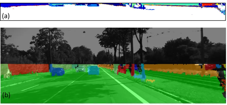
Figure 1.1 Stereo camera system setup. . . 2 Figure 1.2 Methodology for this thesis work. (a) Grayscale image, (b)
Dispar-ity depth map, (c) Robust segmentation results, (d) Multi-objects tracking results, and (e) Flow chart of the proposed methodology. . 3
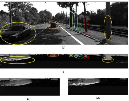
Figure 2.1 Disparity map result. (a) Original gray-scale image, (b) disparity map result, (c) u-disparity map result, (d) disparity map result. In v-disparity map result, the red line indicates the upper plane for road segmentation. . . 17 Figure 2.2 Occupancy grid results. (a) Original gray-scale image, (b) probability
of occupancy grid map, (c) region of probability map for vehicle us-ing approach without equation 2.18 and equation 2.19, (d) region of probability map for vehicle using modified approach which combining eqaution 2.18 and equation 2.19. Plot (d) shows a better probability of detection using the modified approach and in plot (b), (c) and (d), pixels in the middle region of occupancy grid have more dark color which indicate that those pixels has much lower probability for occu-pied by obstacles. This results is contributed by computing occupancy grid combining with road pixels. . . 23
Figure 3.1 Thresholding segmentation result. (a) Thresholding result in u-disparity map, (b) their corresponding regions in image space. . . 27 Figure 3.2 Persistence Analysis. (a) Original grayscale image, (b) images after
thresholding, and (c) persistence diagram. Each point in the diagram corresponds to clusters that are born and die at specific threshold values. Points near the diagonal are sensitive to small variations of the original image. . . 29 Figure 3.3 Birth and death of connected components during filtration. First row
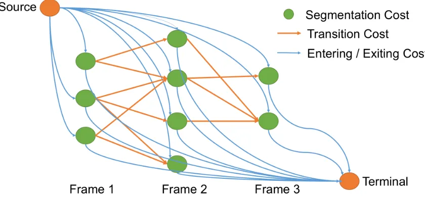
Figure 4.1 Constructed network. Each green spot represents an individual objec-t and segmenobjec-taobjec-tion cosobjec-t geobjec-tobjec-ting from segmenobjec-taobjec-tion algoriobjec-thm. Blue edges represent entering and exiting cost. Yellow edges represent tran-sition cost. . . 37
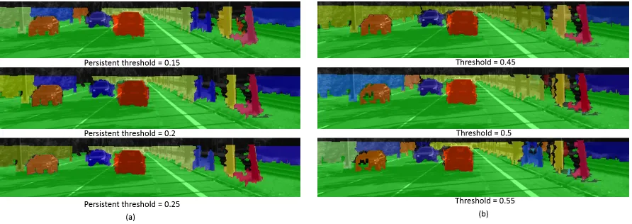
Figure 5.1 Comparison between thresholding and persistence methods. (a) Re-sults of persistence approach forγper = 0.15, 0.2 and 0.25. (b) Results of thresholding approach for τ = 0.45, 0.5 and 0.55. . . 44 Figure 5.2 Changes in detection regions for thresholding approach. (a) Number
of regions added and (b) Number of regions removed as a function of
τ. (c) Total number of regions added or removed. (d) Total number of regions as a function of τ. The bin size for (a)-(c) is 0.05. . . 46 Figure 5.3 Changes in detection regions for persistence approach. (a) Number
of regions removed and (b) total number of regions as a function of
γper. The bin size for (a) is 0.05. . . 47 Figure 5.4 (a) Average number of regions changed for thresholding approach.
(b) Average number of regions changed for persistence approach. (c) Segmentation of thresholding approach for threshold from 0.4 to 0.55. (d) Segmentation of persistence approach for threshold parameter from 0.2 to 0.35. . . 48 Figure 5.5 Segmentation results for persistence bound γper ranging from 0.05 to
0.3. Bushes and trees are separated when γper = 0.05 and 0.1. They are merged whenγper increases from 0.1 to 0.2. Whenγper= 0.25 and 0.3, the results are essentially unchanged. Note that two vehicles are always detected properly for all persistence threshold. . . 50 Figure 5.6 Segmentation results. Results are performed by varying τ ∈[0.1,0.9]
and letting γper = 0.2 in this case. Cars, trees and bushes can be detected and segmented on each frame, and in the first frame we also detected the person on the left side. . . 51 Figure 5.7 Comparison result between tracking method with and without Kalman
filter. (Top) Trajectory length distribution for tracking method com-bined with Kalman filter. (Middle) Trajectory length distribution for tracking method without Kalman filter. (Bottom) Accumulated switch times. . . 53 Figure 5.8 (a) Tracking with Kalman filter using Persistence method. (b)
Introduction
In the past few decades, many researchers have explored the area of intelligent vehicles
and tried to make vehicles perceive and analyze their surrounding environments, in order
to enhance on-road safety. One of the foremost issues that needs to be addressed for
these Advance Driver Assistance Systems (ADAS) is the interpretation of surroundings
of the ego vehicle, i.e. dynamic scene analysis and on-road obstacle detection. However
till data, reliable detection and tracking of obstacles present in front of the moving vehicle
remains one of the most complex task for driver assistance and autonomous navigation
systems. Solution to this problem not only aims for prevention of on-road collisions, but
also builds the basis for further traffic scene analysis. This issue is very challenging for
researchers due to variable illumination conditions, changing weather conditions, highly
dynamic background and limited field of view of the cameras mounted on the ego vehicle.
In this thesis work, we focus on two main problems. The first problem is segmentation
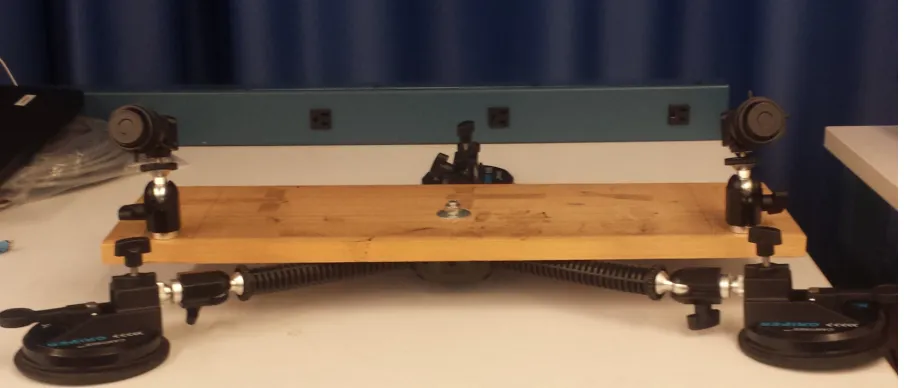
segmentation as input. We construct a stereo camera system, shown in Fig. 1.1 and fix
it on the top of vehicles to capture images simultaneously. Fig. 1.2 provides an overview
of the whole methodology for this thesis work.
Figure 1.1 Stereo camera system setup.
The current state-of-the-art for solving segmentation of obstacles are parameter values
that are carefully selected in order to provide good performance. Often these
parame-ters in fact are threshold values for segmentation of images. However, sensitivity of the
detection results to these parameters can be a big concern. Small changes in threshold
values can lead to large variations in the segmentation of the images. This thesis work
introduces a novel methodology for characterizing the sensitivity of a segmentation result
based on persistent topology, and introduces an approach for robust obstacle detection
In particular, we start with an efficient UV-disparity approach to classify a 3D traffic
scene into a ground plane and obstacles. Then, a visibility based occupancy map is
com-puted to segment the obstacles in the occupancy domain. Finally, we apply a topological
persistence technique on the occupancy map to perform robust obstacle segmentation and
detection. A fundamental difference between our approach and other existing approaches
is its hierarchical nature. Segmentation based on topological persistence does not solely
rely on a single threshold value; instead, it keeps track of all the clustering results,
corre-sponding to different thresholds. This is essentially providing a hierarchical clustering. A
key advantage of our approach over traditional techniques is that the algorithm can be
tuned for better performance through a few intuitive parameters, which leads to results
that are less sensitive than simple thresholding. The proposed method could also provide
us with a persistence diagram, which gives a compact visual representation of
segmen-tation result corresponding to different threshold values. By analyzing this diagram, we
can choose meaningful merging parameters for our segments and can also get a sense of
the stability of the number of clusters under different choice of persistence parameters.
Results of this approach can be found in [Wei14].
And for the tracking problem, traditionally, the problem of multi-object tracking in a
dynamic environment has been performed either by detecting and classifying the targets
in one frame, or tracking those detections in the consecutive frames [Gei13b] [Zha13]; or
by background subtraction methods i.e. tracking by segmenting the moving objects from
the static background [Erb11] [WS11]. In this thesis work, our method extend the works
of [Zha08][Pir11] and incorporate a dynamic programming approach followed by Kalman
frames using network flows. We further improve our algorithm by incorporating a Kalman
filter to estimate the position and velocity of our target objects in the consecutive frames.
Combining the dynamic programming with Kalman filtering reduces the dependence on
the color histogram and the histogram of gradient to find correct matches in consecutive
frames and thus, this approach gives better results in scenarios of variable illumination
conditions, and also performs better to distinguish similar objects, such as trees along the
road. Overall, this tracking approach provides better robustness than traditional tracking
methods based on obstacle segmentation.
My specific contributions to this work include implement the whole procedure for
com-puting occupancy grid map, obstacle segmentation algorithm and multi-target tracking
algorithm and modify the original occupancy grid computation methodology as well as
improve the performance of tracking algorithm by combining features from the
persis-tence topological analysis with features used in the prior literature.
The remainder of this thesis is organized as follows. Chapter 2 gives the obstacle
segmentation approach based on UV-disparity map computations. A brief background
on topological persistence and detailed description of the methodology using persistence
for obstacle segmentation is introduced in chapter 3. In chapter 4, we present a detailed
description of proposed obstacle tracking methodology. Result and experiment
analy-sis of segmentation and tracking method are discussed in chapter 5. Finally, chapter 6
1.1
Literature review
In this section, we will first provide a brief overview of the state-of-the-art of different
segmentation methods, specifically in the field of Advance Driver Assistance Systems
(ADAS). Also, we focus on the current state-of-the-art of stereo vision based approaches,
which make use of disparity depth maps for scene understanding. Then we will provide a
brief overview of the state-of-the-art of different tracking techniques existing in the field
of ADAS.
1.1.1
Segmentation
In [Che10b], Chen et al. segment the stereo disparity map by employing depth slicing
technique and then accurately marking the object boundaries using a region growing
method to improve on-road obstacle segmentation. Another region growing technique
for vehicle detection is suggested by Kormann et al. [Kor10]. In the first step, vehicles,
modeled as cuboids, are detected using mean shift clustering of planar segments. Then
a UV-disparity map is computed to generate hypotheses for vehicle appearance and
disappearance.
Recently, Wang et al. have presented a method for robust obstacle detection and free
space calculation based on efficient disparity map computation and G-disparity [Wan14].
The obstacles are detected using UV-disparity maps, and splines are used for road model.
In [LA12], Lefebvre et al. perform vehicle detection by applying mean shift
segmenta-tion directly on the 3D point cloud, which is estimated from the dense disparity maps
Erbs et al., in [Erb11], compute dynamic stixels from stereo disparity map and use the
Dynamic Stixel World representation for efficient and compact one-dimensional modeling
of real world 3D road scenes. Optimal segmentation is performed by means of iterative
dynamic programming. In [Erb13], this group presents another method for traffic scene
understanding and driver assistance system by incorporating a Bayesian segmentation
approach. Stixel representation of images adds robustness to their algorithms, and thus,
their method works pretty well even in adverse weather conditions.
Determination of a dense disparity map based on-road obstacle detection is presented
as a constrained optimization problem in [Mil07]. The depth image, here, is segmented
based on surface orientation criterion. In [GB06], two new obstacle detection algorithms
based on disparity map segmentation for applications in intelligent vehicle systems are
presented. The first algorithm assumes that the obstacles are located almost parallel to
the image plane and directly segments them using a robust model fitting method applied
to the quantized disparity space. The second method employs some morphological
oper-ations and followed by a robust model fitting technique to separate the ground regions.
Lee et al., in [Lee11a], perform vehicle detection using a road feature and disparity
histogram. Road features are extracted from v-disparity maps and localized obstacles
are divided into multiple obstacles using a disparity histogram, and remerged using four
criteria parameters : the obstacle size, distance, angle between the divided obstacles, and
the difference of disparity values. In [Lee11b], they present another stereo-vision based
obstacle detection approach using UV-disparity map and birdeye view mapping.
Recently, map-based segmentation and navigation techniques for autonomous vehicles
based on probabilistic and heuristic methods to classify and predict the areas around
an autonomous robot. Another path planning method for mobile robots is presented in
[Che10a]. This paper employs an enhanced dynamic Delaunay Triangulation approach
and a GPS tail technique for robot navigation. In [Pos11], Posada et al. present a robust
method of floor-obstacle segmentation for mobile robot navigation. The method relies on
fusing opinions of multiple heterogeneous classifiers generated from different segmentation
schemes like graph cut and region growing to improve the overall classification rate.
Some other papers on traffic scene analysis and obstacle detection have incorporated
techniques like watershed segmentation [Vei09]. Connected component analysis [Kha13],
plane-fitting and edge based segmentations [Li04]. Literature has also addressed several
surveys on intelligent transportation systems [ST13], [Had14].
1.1.2
Tracking
In literature, the problem of object tracking from moving platforms using optical sensors
has mainly been categorized into monocular and stereo vision based approaches. Recently,
fusing monocular and stereo vision has also gained popularity [ST11]. Because this thesis
work focuses on stereo-based approach, the following section will pay more attention to
stereo-based tracking methods.
Target tracking in ADAS using stereo vision mainly deals with estimating the position
and velocity of different obstacles on the road. Estimation is most commonly implemented
using Kalman filtering [Fra05], which assumes linear motion and Gaussian noise. However,
as these on-road motions in reality are usually non-linear, using Extended Kalman filter
This section details some of these common object tracking methods which are prevalent
in research literature.
Many approaches first segment the moving objects from ground using different
back-ground subtraction techniques and then these detected foreback-ground regions are analyzed
and tracked [Bad07][Kla08]. In [Erb11], Erbs et al. concentrated on the segmentation of
space-time data obtained from stereo image sequences. The proposed object detection
approach changes the Stixel labeling decision between a moving object and the
station-ary background into a hypotheses testing problem. Segmented regions are tracked over
frames using Kalman Filters i.e. the velocity for dynamic Stixels is estimated by Kalman
filtering a representative velocity vector of this Stixel patch over time.
Other approaches detect and classify objects in different classes, and then, track these
objects in consecutive frames. In [Gei13b][Zha13][Gei13a], the authors present a novel
probabilistic generative model for multi-object traffic scene understanding from movable
platforms. The basic method followed is Tracking-by-Detection. Tracking operates in the
following stages : object detection in each frame independently using the DPM object
detector [Fel10]; detections with positive score associated to detctions in the next frame
using appearance and the bounding box overlap; prediction performed using a Kalman
filter; and detections between consecutive frames associated via the Hungarian method
[Kuh55] for bipartite matching.
Lenz et al. propose a sparse scene flow based class-independent method in [Len11] for
detecting moving objects in inner city traffic scenarios. Their algorithm uses
computa-tionally efficient sparse interest points in consecutive stereo images to compute the scene
independently moving rigid objects in the scene. Due to the class-independent nature,
this method works better in scenarios where appearance-based object detectors.
In [Kwo10], Kwon et al. present a dense stereo vision based obstacle detection and
tracking method by combining a global stereo matcher with a correlation based cost
function for generating a reliable disparity-map. A normalized cross correlation (NCC)
algorithm is used to make the approach efficient in case of illumination variation and
texture-less areas in real driving scenarios.
Another stereo vision based obstacle extraction method is proposed in [Sug09]. The
novelty of the approach lies in choosing a shorter baseline for the stereo vision system
than the general ones so that the room mirror where the system is mounted can cover
it. Traditional ”V-Disparity” approach is extended to a more flexible system by using
Virtual Disparity Image. By using virtual disparity image (VDI), obstacles are extracted
simply and robustly. By using road surface appearance and shape information as object
clustering algorithm, objects are correctly clustered in more complex situation. Clustered
objects excepting too small or too big objects are tracked by using Extended Kalman
Filter (EKF) to estimate its distance and velocity robustly.
The target objects are modeled by a rigid 3-D point cloud in [BF09] by Barth et al.
This point cloud is tracked in an image sequence in terms of feature displacements and
depth measurements from the stereo system. An extended Kalman filter is then used to
relate the observations in the image to a 3-D object movement.
In [Sun10], a scale invariant feature transform (SIFT) based particle filter algorithm
is presented for joint detection and tracking of independently moving objects in stereo
novel multi-view matching method is proposed for simultaneous stereo matching and
motion tracking of the detected features. A multi-view geometric constraint, derived
from the relative camera positions in pairs of consecutive stereo views, is then derived for
independent motion detection. Finally, a dimensional variable particle filter is introduced
for detection of joint and tracking of multiple independently moving objects.
Arrospide et al. in [Arr10] proposed method exploits the geometrical relations between
the elements of the scene for vehicle detection, so that moving objects can be detected by
analyzing motion parallax. A novel probabilistic framework based on Kalman filtering is
presented for reliable and accurate homography estimation. The estimated homography
is used for image alignment, which in turn allows detecting the moving vehicles in the
image. Tracking of vehicles is performed on the basis of a multidimensional particle filter,
which also manages the exit and entries of objects.
In [Moq11], a new method for detecting and tracking objects using stereo vision with
linear cameras is presented. Edge points are first extracted from the linear images and
are matched to obtain the reconstructed points representing the objects in the scene.
These points are then segmented in order to form clusters, where each cluster of points
corresponds to an object of the scene (spectral/k-means clustering). The detected objects
are tracked throughout the centers of gravity of the extracted clusters using Kalman
filtering and a nearest neighbor based data association technique.
Mean Shift algorithm [LA12] is applied to simultaneously extract each vehicle and
track the 3D points belonging to the same vehicle along the sequence. It is shown that
several vehicles can be efficiently detected and that a semi-dense disparity map is sufficient
to mean shift segmentation process using Kalman filter.
[Lat11] provides a grid-based mapping method designed for static environments with
object tracking. The stationary part is fused in our static grid whereas moving parts are
tracked yielding reliable motion estimates. The classifier used to distinguish moving from
stationary parts is based on a Sequential Probability Ratio Test (SPRT), a model selection
method which blends well into the tracking architecture. Tracking is implemented using
Extended Kalman filtering.
The dynamic environment of a typical driving scene is tracked as an occupancy grid
based on particle filtering in [Dan11]. The occupancy grid tracking solution presented in
this paper can be classified as having a Cartesian representation, using a forward sensor
probability model, and producing a fully dynamic grid.
In [She11], the authors present an efficient stereo vision based system that is capable
of detecting and tracking objects in full range and wide FOV for both short and long
range applications. The object tracking module estimates the kinematics and geometric
features of detected objects using joint probabilistic data association and multi-model
tracking techniques. The detected objects are statistically associated with existing tracks,
and their states are updated by the measured down range, cross range, width, depth, and
height.
Lim et al. explain a tracking-by-multiple hypotheses framework [Lim13] consisting
of obstacle detection, vehicle recognition, visual tracking, global position tracking, data
association and particle filtering. Global position tracking estimates the position and
velocity of a target object on the road using a stereo vision system. The accuracy of
estimation is very important in estimating the distance accurately and precisely. The
IPM-based EKF method reduces the error covariance of the position and velocity of the
target. The 3D feature based visual tracking module consists of feature extraction, feature
tracking, feature selection, 3D feature clustering, model selection and ROI estimation.
Due to its speed and high repeatability, a feature from an accelerated segment test (FAST)
detector is used to extract distinctive features.
A new method for vehicle detection and tracking based on stereo vision, motion
anal-ysis and road detection is presented in [MM11]. The road detection with motion
segmen-tation, considering a parallax in stereo vision as a motion, enables on-road vehicle and
obstacle detection. All elements constructing the proposed method are founded
common-ly on affine motion segmentation, which uses affine motion model to merge pixels into a
region. Object tracking with motion estimation, which follows the next object detection
starting with an initial solution given by the tracking, improves detection accuracy.
In [Pir11], multi-object tracking problem is formulated in a minimum cost flow
frame-work. A dynamic programming approach based on greedy algorithm is employed to attain
a global solution. This method basically works by sequentially instantiating tracks using
shortest path computations on a flow network. Zhang et al. propose another network
flow based optimization method for data association needed for multiple object tracking
[Zha08]. The frames are associated optimally by a min-cost flow algorithm in the network.
Occlusion is handled by constructing an Explicit Occlusion Model (EOM).
Andriyenko et al. in [And12] approaches the issue of multi-target tracking by jointly
addressing data association and trajectory estimation problem by minimizing a consistent
by performing minimization of continuous energy in order to attain global optimality. In
contrast to their previous contribution, the objective function is designed in a more robust
manner so that the energy function takes into account physical constraints, such as target
dynamics, mutual exclusion, and track persistence.
Research is also on-going for tracking objects from mobile platforms in
differen-t unfavorable driving scenarios, for example, in bad weadifferen-ther and low-lighdifferen-t condidifferen-tions
[Fos11][O’m11], near turning lanes [BF10] and intersections [Bar09]. Literature has
al-so addressed several surveys on moving target tracking in the field of ADAS, such as
Occupancy Grid Computation
This chapter presents the whole approach for occupancy grid computation, starting with
basic concepts from disparity map computation. Then we show the algorithm for
com-puting grid computation in detail. The final section will demonstrate improvement and
optimization for robust results. This work has been published and details can be found
at [Wei14].
2.1
UV-disparity Map
In this section, we start with a disparity map which has been computed from a stereo pair
of images from the vehicle based on theSemi Global Block Matching (SGBM) technique
[Hir08]. A disparity map can be represented as a 3D point cloud where each point has
coordinates (u, v, d), where (u, v) represent thex-ycoordinates in the image domain and
concept we know that based on the disparity valuedof point p, we can retrieve the point location in both left and right image, which should be xl = (u, v) andxr = (u−d, v). If we assume that after calibration, the yaw, pitch and roll angles of cameras are set to zero
and based on the transform function, we are able to re-calculate the world coordinates
of point P based on point pin disparity map, which shows below given by [Per10a]:
u=u0+au· zW
−x0−bs/2 yW−y0
v =v0+av· yzWW−−zy00
d=au·yWb−sy0
(2.1)
where (x0, y0, z0) is the coordinate for the center of stereo camera system, au and av represent the intrinsic focal length parameters of left camera in pixels and bs is the distance of the baseline for the stereo camera system. Then by projecting all the points
in the disparity map to the ud-plane and vd-plane and accumulating the overlapping points, we can generate two new 2D images, called the u-disparity map and v-disparity
map [HU05] respectively. U-disparity map and v-disparity map are complementary results
and for u-disparity map, the result is like a bird-eye view representation of scenes in
disparity map. Fig. 2.1 (a) shows the left original image for a stereo pair images we used
for testing and Fig. 2.1 (b), (c) and (d) illustrate the correspondence disparity, u-disparity
and v-disparity map respectively.
2.2
Road Segmentation
ob-Figure 2.1 Disparity map result. (a) Original gray-scale image, (b) disparity map result, (c) u-disparity map result, (d) v-disparity map result. In v-disparity map result, the red line indicates the upper plane for road segmentation.
plane, then every row of disparity map that intercepts the road will have its smallest
value at the road pixels. That is, the points in the v-disparity map will have as lower
bounded by the points associated with the road. This lower bound can be approximated
by a line in the v-disparity map.
While due to the noise and some wrong value points in the disparity map, the lowest
point for each column in v-disparity map may not represent road pixel. In order to obtain
a robust estimate for the ground plane, a line is fit to the v-disparity map using robust
regression techniques [Str88]. The basic idea for robust regression algorithm is to solve a
weighted least squares problem by iterative method which has the following form:
argmin β
n
X
i=1
|yi−fi(β)|p (2.2) and parameter β updated by:
β(t+1) = argmin β
n
X
i=1
To be more specific, in our situation all points only have two dimensions information, so
the parameter β = (β1, β2)T, and
argmin β
ky−Xβk2 = argmin β
n
X
i=1
|yi−Xiβ|2 (2.4) where n is the number of column in the v-disparity map, Xi = (di,1) represent the disparity value for each points in the v-disparity map andyi =vi shows thev coordinate value for the correspondence point. Then we update parameter β using the following equation:
β(t+1) = argmin β
n
X
i=1
ωi(t)|yi−Xiβ(t))|2 = (XTW(t)X)−1XTWty (2.5)
where W is a diagonal matrix of weights and ωi(0) = 1. We update W using equation 2.6 for each iteration, and for each outlier points, the weight for them will decrease that
finally we can rule out outliers.
ωi(t) = 1
max(δ,|yi−Xiβ(t)|)
(2.6)
where δ is a small number.
After getting the fitting result, this line is referred to as gground(d). Now we are able to calculate the lowest position vi for each disparity value di using gground(d). Then by applying an appropriate threshold (based on height) for all points in the disparity map,
we could segment the road and obstacle pixels in the original image domain. In particular,
glower(d) = gground(d) +
auhg
avbs
(2.7)
where hg is the height above the estimated ground plane used to identify road pixels,
au, av and bs are the same as equation 2.1. Fig. 2.1 shows glower as a red line in the v-disparity map result.
2.3
Occupancy Grid Computation
An occupancy grid is a probability map where each cell in the grid represents the
prob-ability of that cell, which is occupied by an obstacle. In this thesis work, we compute an
occupancy grid in the u-disparity map following the idea of [Per10b], in order to enable
the segmentation of objects. The whole procedure can be divided into two parts. First,
we obtain an occupancy map by using only those points in the disparity map that are
above the ground plane while below a plane of height hmax, which specifies a maximum detection height in this approach. Then we use the road pixels we have obtained in the
above section to improve the resulting robustness of the occupancy grid.
2.3.1
Occupancy grid based on obstacle pixels
P(Os) =
X
v,c
P(Vs=v, Cs =c)·P(Os|Vs=v, Cs=c). (2.8)
We can assume that visibility and obstacle confidence are independent with each
other, and v ∈ {0,1}, c∈ {0,1}, then we can rewrite equation 2.8 as follow:
P(Os) =
X
v=0,1
X
c=0,1
P(Vs =v)·P(Cs =c)·P(Os|Vs=v, Cs=c). (2.9)
P(Os|Vs = v, Cs = c) represents the conditional probability of occupancy given vis-ibility, and obstacle confidence. We show the expression of this conditional probability
under three different condition, as
P(Os|Vs = 0, Cs=c) = 0.5 ∀c∈ {0,1}
P(Os|Vs = 1, Cs = 1) = 1−PF P
P(Os|Vs = 1, Cs = 0) = PF N
(2.10)
with PF P and PF N representing the false positive and false negative probabilities of occupancy detection respectively. We can then modify the equation 2.9 as follow,
P(Os) =P(Vs= 1)·P(Cs= 1)·(1−PF P)+P(Vs = 1)·(1−P(Cs= 1))·PF N+(1−P(Vs= 1))·0.5 (2.11)
Now we need to give the expressions for P(Vs = v) and P(Cs = c). In order to compute these probabilities, we define three new variables NP(s), NO(s) and NV(s).
the total number of obstacle points at that site and NV(s) is the total number of visible points for site s.
As we have mentioned before, we have defined a maximum detection plane height
hmax, so for a given site s in the occupancy grid, the total number of measured points is
NP(s) = gupper(d)−glower(d) (2.12) where glower(d) is the v-coordinate for ground plane we use for segmenting ground with obstacles, andgupper(d) is the v-coordinate for the maximum heighthmax plane. By using equation 2.1, we can obtain the following equation,
gupper(d)−glower(d) =
au
av
· hmax·d
bs
(2.13)
ForNO(s), we need to count the number of points belongs to the range [glower(sd), gupper(sd)] that has disparity value equals to sd. And for NV(s), we need to count the number of points in the same range that has disparity value great than 0 as well as smaller or equals
to sd. If a point for site s has disparity value larger than sd, the point is occluded by other obstacles. To summary, we have the following equations,
AP(s) = {(u, v)|u=su, v∈[glower(sd), gupper(sd)]}
AO(s) ={(u, v)|ID(u, v) =sd} ∩AP(s)
AV(s) ={(u, v)|ID(u, v)≤sd} ∩AP(s)
Na(s) = |Aa(s)|, a∈ {P, O, V}
(2.14)
ratio of the total number of measured pixels and the total number of visible pixels
P(Vs = 1) =
NV(s)
NP(s)
(2.15)
and then we define a confidence ratio α as
α= NO(s)
NV(s)
(2.16)
which means that if more pixels belong to visible pixels then they can be grouped as
obstacle pixels, we should have a higher confidence for an observable obstacle. And this
lead to the expression of the probability of confidence of observation
P(Cs= 1) = 1−e−λα (2.17) where λ is a constant parameter. Fig. 2.2 shows the probability of occupancy grid re-sults and highlights some corresponding regions in between the grayscale image and the
occupancy map.
A scenario in which this approach does not seem to work that well is, when surfaces
of the obstacles observed are not vertical (e.g., the windshield of a vehicle). In this case,
points of the same object are dispersed over various sites on the u-disparity map, which
leads to low probability of occupancy over a region in this space.
To resolve this problem, all the invisible points in the disparity space below a point
that has already been identified as an obstacle are considered as obstacles. In other words,
Figure 2.2 Occupancy grid results. (a) Original gray-scale image, (b) probability of occu-pancy grid map, (c) region of probability map for vehicle using approach without equation 2.18 and equation 2.19, (d) region of probability map for vehicle using modified approach which combining eqaution 2.18 and equation 2.19. Plot (d) shows a better probability of detection using the modified approach and in plot (b), (c) and (d), pixels in the middle re-gion of occupancy grid have more dark color which indicate that those pixels has much lower probability for occupied by obstacles. This results is contributed by computing occupancy grid combining with road pixels.
we redefine
AnewO (s) =AO(s)∪(AIO(s)∩AP(s)) (2.19) and use this quantity to update the value of NO(s). Fig. 2.2 (c) and (d) show the im-provement on the probability of occupancy by coupling the above equations.
2.3.2
Occupancy Grid Improvement using Road Pixels
We can use road pixels to improve the quality of occupancy grid. Now we need to define
two new probabilities, the probability of final occupancy grid P(Fs) and the probability represent a site s only belongs to the road surfaceP(Rs). Then we can define
P(Fs) = P(Os)·(1−P(Rs)) (2.20) Unlike counting accumulate number of pixels for calculating theNV(s) andNO(s), we do not accumulate road pixel in u-disparity, because road pixels are not always vertically
aligned. Instead, we measure the number of road pixels in the neighborhood of each site
s. We define a road confidence ratio β as the ratio of non-zeros road pixels in a fixed size neighborhood of site s, in this thesis work, we use a 3×3 neighborhood. Then we can define
relative high confidence being considered as an obstalce, the probability that it can be
considered as road should be low and vice versa is also true. In Fig. 2.2 (b), (c) and (d),
pixels in the middle region of occupancy grid have darker color which indicate that those
pixels has much lower probability for occupied by obstacles. These results are obtained
Obstacle Segmentation Algorithm
3.1
Obstacle Segmentation by Threshold Value
The traditional approach for obstacle segmentation in the u-disparity domain is to apply
a constant threshold to the occupancy grid and form a new binary map. Then we apply
a connected component algorithm for this binary map and all connected components can
be regarded as separate obstacles.
Each obstacle detected in the u-disparity domain needs to be mapped back to the
original image plane for display. Given a site s in the u-disparity space, we identify all points in the disparity map with u-coordinate su and disparity value sd. Then we label the correspondence pixels in image domain as the same obstacle label as site s. Fig. 3.1 illustrates the segmentation result for thresholding method which value set as
Figure 3.1 Thresholding segmentation result. (a) Thresholding result in u-disparity map, (b) their corresponding regions in image space.
3.2
Obstacle Segmentation using Topological
Persis-tence
Topological Data Analysis [Ede02] is a new field of study which employs tools from
persistent homology theory [EH08]. This analysis is commonly used for the extraction of
topological attributes from functions or point cloud data. These features are captured in a
compact visual representation called the persistence diagram [EH10]. Persistent homology
has been used for segmentation [LF07] of natural images and clustering [Cha13]. In this
thesis work, we make use of persistence analysis to fulfill the robustness of obstacle
detection. In the first section we will provide a brief introduction of some key concepts
demonstrate how to apply topological persistence analysis to segment obstacles in our
algorithm.
3.2.1
Topological Data Analysis
First, let us consider a function f : R2 → [0,1]. Given a threshold value τ ∈ [0,1], we compute the upper level set Sτ = f−1[1−τ,1]. In this thesis work, f represents the probability of obstacle occupancy at a location in front of the ego vehicle and Sτ represents a set of result of detections by tradition threshold method that we use τ
as the threshold value. The goal for topological persistence analysis is to analyze these
detections and characterize their sensitivity to the threshold value τ.
The topological structures of the setSτ ⊂R2can be summarized using theBetti numbers, which are the ranks of topological invariants calledhomology groups. Then-th Betti num-ber,βn measures the number ofn-dimensional cycles in the space (e.g., for a 2D space,β0 is equal to the number of connected components and β1 is equal to the number of holes in the space). The set {Sτ}τ⊆[0,1] is referred to as a filtration and satisfies the following property:
Sτ1 ⊆Sτ2 whenever τ1 ≤τ2 (3.1)
Persistent homology computes the values of τ for which topological features appear (bk
into a multi-set of points (bk
n, dkn), called a persistence diagram. Each point is referred to as a persistence interval with corresponding length equal to dk
n−bkn. Algorithms for the efficient computation of persistent homology can be found in [Ede02], [ZC05].
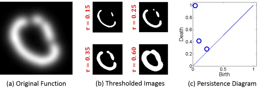
Figure 3.2 Persistence Analysis. (a) Original grayscale image, (b) images after thresholding, and (c) persistence diagram. Each point in the diagram corresponds to clusters that are born and die at specific threshold values. Points near the diagonal are sensitive to small variations of the original image.
An example of a function f, sample sets Sτ, and persistence diagram (for n = 0) is shown in Fig. 3.2. At τ = 0.15, there exists two connected components, which split the ring into two parts. A small connected component, the small dot at the top of the ring, is
born atτ = 0.25. When τ = 0.35, the small dot born atτ = 0.25 dies, because it merges with another connected component which has an earlier birth time. This situation leads
earliest birth time. Then, a persistence diagram which encodes the birth and death time
of each region can be used to select the persistent region. The diagram corresponding to
this example is shown in Fig. 3.2 (c). The further away a feature is from the diagonal,
the higher is its persistence and robustness to perturbations.
3.2.2
Obstacle Segmentation via Persistence Diagram Analysis
Let us begin by defining
f(s) = P(Fs) (3.2)
as the probability of occupancy function computing using both obstacle pixels and road
pixels over the u-disparity space in order to draw a connection with the concepts
intro-duced in section 3.2.1.
Segmentation of f via simple thresholding is fast and easy to implement, as we have declared in section 3.1. However, the proper threshold value may not be easily selected due
to variations on the probability map attributed to the quality of the disparity map. The
latter is affected by external and internal factors such as illumination and the texture of
objects. Object with less texture features leads to bad disparity map result and improving
the quality of the disparity map always means increasing the complexity of disparity map
computation.
Thus, the ideal threshold may change between images, even in the same video
se-quence. This simple type of segmentation is very sensitive to the choice of threshold
ana-value in the later chapter. Furthermore, obstacles are associated with peaks in
probabil-ity of the occupancy map f, for which there may not be a single threshold value, which includes all these peaks without merging obstacle regions that are not supposed to be
merged. In order to address all of these issues, we make use of topological persistence to
generate a more robust segmentation.
Fig. 3.3 (upper) illustrates the birth and death process of connected components
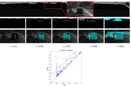
during the filtration of upper level sets off. Atτ = 0.2, the cyan region is born. Another region in red is also born at τ = 0.24 but dies at τ = 0.25, because it merges with the cyan region, which has an earlier birth time. The persistence interval of the red region
is 0.01. At τ = 0.49, the cyan region is still alive and its area increases. At τ = 0.64, this region dies leading to a persistence interval of length 0.44. Note that by choosing
regions with a persistence interval length greater than γper = 0.2, the cyan region would be selected, while the red region would be removed.
The birth and death of all regions obtained from f are captured in the persistence diagram, as displayed in Fig. 3.3 (lower). Each point in the persistence diagram represent
the lifespan of a region. Note that this diagram contains hierarchical information about
the merging of these region as a function of threshold valueτ. In order to obtain a robust segmentation of the obstacles, we keep only those regions with persistence interval greater
thanγper = 0.2. This bound is illustrated by a red line in Fig. 3.3 (right). Finally, in order to obtain a labeling of the clusters in the u-disparity map, we need to determine the
support of the selected persistent regions. However, since a region can exist over a range
Figure 3.3 Birth and death of connected components during filtration. First row on the left shows a part of the original image and the corresponding probability of occupancy map. Sec-ond row shows a connected component in cyan which correspSec-onds to a car in the image s-pace for five different values ofτ, and third row shows the corresponding regions in image space. On the right, the persistence diagram corresponding to the shown occupancy map. Each point indicates the lifespan of a connected component. The red line is the threshold line
γper = 0.2. All the regions above this line have persistence interval greater than 0.2.
by using the above strategy for determining the obstacles region is that the support of
the regions may be overlapping. To deal with this problem, we assign the overlap point
in u-disparity space to the region with the earliest death time, which can be regarded as
a split represent strategy.
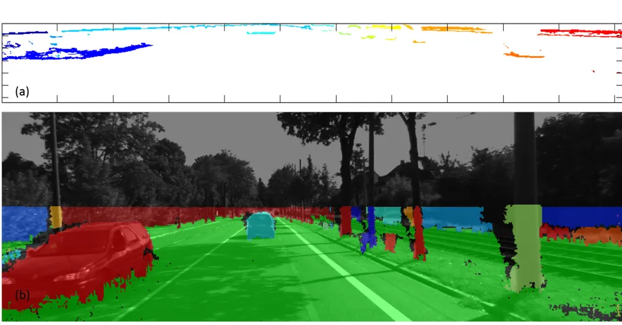
Figure 3.4 Persistence diagram analysis segmentation results. (a) Clusters in u-disparity space, and (b) their corresponding regions in image space.
introduced in section 3.1 to illustrate the segmentation result in the image domain. One
advantage of the persistence diagram is its stability property [CS07]. Small changes in
the functionf lead to small changes in the persistence diagram. This translation into the following for the thesis work scenario: we can obtain segmentation result that is robust
to parameter value changes and small variations in the disparity map. These results will
Tracking Methodology
In this thesis work, we adapt the tracking technique introduced in [Zha08][Pir11]. Data
association is done using network flows [Zha08] and then the maximum flow problem
is solved using global greedy [Pir11] algorithm. We first construct a Hidden Markov
Model (HMM) based flow network using prior works from [Zha08]. In each frame, the
segmented objects are represented as vertices of the flow network. Edges between every
pair of vertices represent the cost for considering two objects belonging to the same
trajectory. After the whole network is constructed, this thesis work combines a dynamic
programming approach with a Kalman filter to solve the multi-target tracking problem.
4.1
Network Flows Model
In this section, we provide details about the construction of the network flows for our
tracking problem based on the prior work [Zha08].
segmentation results. In this set, each objectoi is a vector containing information about the state of the object, such that,oi ={xi, ti, ai}, wherexi represents the location of an object, ti represents the birth (bi0) and death (di0) time of that object in the persistence diagram corresponding to a particular frame, and ai contains information about the appearance of the object, i.e., in this thesis work, we use color histogram and histogram
of gradient to represent objects appearance features.
We then define another set T ={Tj}, which is the set of trajectories. Every element
Tj ∈ T represents a tracking trajectory and Tj can be represented as an ordered list of objects, such as, Tj ={oj1, oj2,· · · , ojn}.
The objective of the network flows model is to maximize a posteriori probability
(MAP) of T given the segmentation result set O. We can express it as:
Tr = argmax T
P(T|O) = argmax T
P(O|T)P(T). (4.1) Then we can assume that the probability of each object, oj, is conditionally independent given a trajectory Tj. Moreover, it is evident that under real tracking scenarios, every segmented object can be treated as part of only one trajectory. This imposes the flow
network constraint that the intersection between two different trajectories must always be
null. Also, we can assume that every object in a frame is independent and each trajectory
is independent. Under these assumptions, equation 4.1 can be simplified to:
Tr= argmax T
Y
j
P(Tj)
Y
i
Tm
\
Tn=∅,∀m 6=n. (4.3) In the above equation,P(oi|T) is the probability that indicates robustness and accuracy of our segmentation results. This term will be discussed later. P(Tj) can be written as
P(Tj) = Pe2P(oj1, oj2)P(oj2, oj3)...P(ojn−1, ojn) (4.4) where Pe is the entering and exiting probability for objects, P(ojm−1, ojm) is the link probability between two segmented objects. We modify equation 4.2 by incorporating
logarithmic indicators,
Tr = argmin T
−
X
j
log(P(Tj)) +
X
i
log(P(oi|T))
(4.5)
Tr= argmin T
X
j
Ce+
X
i
Ci+
X m,n Cm,n (4.6) where
Ce=−log(Pe2) (4.7)
Ci =−log(P(oi|T)) (4.8)
Cm,n =−log(P(om, on)). (4.9) From the above equations, we construct a network representing all possible objects as
of tracking problem constraint, each edges in the flow network should have unit flow, for
each object can be part of only one trajectory.
Figure 4.1 Constructed network. Each green spot represents an individual object and seg-mentation cost getting from segseg-mentation algorithm. Blue edges represent entering and exit-ing cost. Yellow edges represent transition cost.
4.2
Min Cost Algorithm
To calculate the shortest path in a network, we modify the works cited in [Pir11]. In
[Pir11], Pirsiavash et al. have used a DPM object detector [Fel10] to detect objects in
each frame and each object is assigned a unique score. In this thesis work, we detect the
objects in each frame from the persistence based segmentation method and modified the
In this section, we first define each cost term used in equation 4.6. Ce is the entering and exiting cost for the trajectories. For simplification, in this thesis work, we set Ce to be a constant number for all segmentation objects. However, to model more complicated
behaviors of trajectories, Ce can be set according to some information, such as location information, to model the entering and exiting position for most trajectories should near
to the boundary of images.Ci represents the score associated with our detections in each frames and provides us with a measure for robustness and accuracy of our segmentation
results. We have calculated Ci as follows:
Ci =β−α(birth(oi)−death(oi)), (4.10) where (birth(oi) −death(oi)) represents the life time of the object in the persistence diagram, and α and β are two constant coefficients.
Cm,n represents the transition cost between objects m and n in a trajectory. In this thesis work, we use RGB color histogram and histogram of gradient (HoG) of
gray-scale images as the appearance model for each object. Cm,n is defined based on the
Bhattacharyya Distance of the color histogram and HoG between objects,
Cm,n =−ln
γ1
X
x∈X
p
om(cx)on(cx) +γ2
X
y∈Y
q
om(HoGy)on(HoGy)
, (4.11)
gray-scale image for object m.
The segmentation cost Ci can be a negative value; however, Ce and Cm,n are always positive.
Instead of solving the max flow network problem using the push-relabeling method
[Zha08], we use an iterative dynamic programming method [Pir11] to compute one
tra-jectory in each iteration. In each iteration, we always start computing from the object
having lower frame index. First, we initialize the current cost Cc(i) for each object oi:
Cc(i) = Ci+Ce. (4.12) Then, for each objectoi , we find an object setJ ={oj}such that each object in this set has a potential transition with objectoi and the frame index ofoj is smaller than the frame index of oi. In the next step, we use the following equation to update the current cost Cc(i):
Cc(i) = Ci+min(CJ, Ce) (4.13) where
CJ =min(Cj,i+Cc(j) +σ·(f rame(j)−f rame(i))) (4.14) In equation 4.14, σ is a constant number and the third term in this equation model missing objects in consecutive frames based on distance of gaps.
element of our current computed trajectory. We can trace back along that trajectory to
get the whole set of objects belongs to this trajectory. Once we record information of
that trajectory, we remove all the objects and the corresponding edges connecting with
them in the network. We then repeat the whole procedure iteratively until there remains
no more vertex in the network or the minimum cost of current computed trajectory is
above a fixed threshold value.
4.3
DP with Kalman filter and Neural Network
Although the method stated above cannot ensure that the results match exactly with
the real max flow solution, the complexity of the method decreases from O(N3log2N) [Zha08] toO(KN) [Pir11], whereK is the optimal number of unique tracks and N is the length of the video sequence, with minor performance difference. The proposed algorithm
still has several shortcomings. Firstly, it does not incorporate any location information
in the transition costs and the distance information between two objects alone cannot
always provide robust information for tracking. Secondly, the vision system is mounted
on a mobile platform, and thus, the lighting conditions vary hugely between frames. This
reduces the performance efficiency of the color histogram. Thirdly, the input data for
our tracking algorithm is the basic segmentation result and not from any classification
algorithm. As a result, our input contains both foreground and background objects,
making the tracking even more difficult.
To overcome these problems, we extend the original approach stated in the above
locations for the object oi are obtained using a Kalman filter state vector stored in objects oj. Finally, update the current cost Cc(i) as follows:
Cc(i) = Cc(i) +|xi−xˆi| −τ. (4.15) Here, xi is the real position of oi, ˆxi is the prediction position of oi from oj and τ is a constant number.
We also construct a two layered neural network using Levenberg-Marquardt
back-propagation algorithm [HM94] to update the weight and bias of each object. Inputs of
the neural network are normalized RGB color histogram of the objects, represented as
24×1 vectors. Number of neurons for inner layers of the neural network is set to 100, and the output layers have dimension one. We manually label 3590 objects from the
persistence based segmentation method using different image sequences as training data
set.
Inputs for our tracking algorithm come from a segmentation algorithm and not from
any object detection-by-classification algorithm. This means our inputs contain the
fore-ground objects, i.e. the obstacles, as well as the backfore-ground objects. Objects belonging to
the background sometimes have longer life time in the persistence diagram and thus, can
be easily tracked. This situation can decreased the performance of our tracking
algorith-m. The pre-trained neural network helps us to improve the performance of our algorithm
by distinguishing the foreground objects from the background. Instead of eliminating the
background information before tracking, after each iteration, we apply the neural
net-work to all the objects present in the most current trajectory and count the number of
than a preset threshold value, we treat this trajectory as a false trajectory, eliminate all
the background objects along with the edges connecting them in the network and keep
computing the next trajectory. The reason for adopting this strategy is because if the
neural network performance is not good enough at a single frame, sometimes it labels
some foreground objects as the background and as a consequence, gaps are created in
Experiment
This chapter contains two different experiments. In the first experiment, we focus on the
segmentation algorithm based on topological persistence analysis, which are compared
against segmentation result via tradition threshold method. In the second experiment,
we pay attention at tracking algorithm mentioned at chapter 3 to show efficiency and
robustness of our tracking algorithm which incorporate our robust segmentation method
based on persistence diagram analysis. The whole experiment make use of stereo image
pairs from the KITTI Vision Benchmark Suite [Gei13c], [Gei12], [Fri13] for analysis.
5.1
Experiment for segmentation algorithm
The entire process is implemented in MATLAB on a 2.4 GHz dual-core laptop with
16GB RAM. It takes approximately 13.76 seconds for a 1242 × 375 image for τ ∈
unless otherwise specified. For both the thresholding method and the proposed persistence
diagram analysis method, a simple morphological post-processing step is applied to the
segmented images in order to remove the small detection regions as well as the small
gaps in the detection regions. In this section, we compare the persistence method with
the traditional thresholding method and analyze the effect of persistence bound for the
proposed persistence diagram analysis method.
5.1.1
Comparing Threshold and Persistence Method
Although thresholding is a simple solution for segmentation of the obstacles using the
probability of occupancy map, it is highly sensitive to the choice of parameter value. On
the other hand, the persistence based method performs an analysis for a range of threshold
values and keeps track of all the resulting segmentations in a hierarchical fashion. We
exploit this property to obtain a more robust outcome.
Fig. 5.1 provides sample results for both the thresholding and persistence methods.
For thresholding, τ is set to 0.45, 0.5 and 0.55 respectively. For persistence, γper is set to 0.15, 0.2 and 0.25 respectively. We pick these ranges in order to make the results for
both methods comparable for the middle parameter value and in the most occasions,
parameter around the middle parameter value can provide a relative good result for both
segmentation methods. It is observed that even over this small range, for here is 0.1,
thresholding causes significant variation in its output. In particular, there are several
detection regions that appear and disappear on the right side of the image. On the
contrary, the results for persistence are very consistent over a similar range of parameters
and the shape for each detected region is almost the same.
We quantify the robustness of our method by analyzing how many new regions are
in-troduced and how many old regions are removed as parameters change for both methods.
Fig. 5.2(a) and (b) illustrate how regions get added and removed by using the
threshold-ing approach. These plots are histograms of the birth and death values of all the regions
computed from the persistence analysis. Fig. 5.2(c) represents the total change on the
number of regions as a function of threshold parameter τ. When τ changes from 0.45 to 0.5, around 30 regions are added or removed from the result, some of which are removed through post-processing that not be highlighted on the segmentation result image. When
τ changes from 0.5 to 0.55, around 20 regions are added or removed. Fig. 5.2(d) shows the total number of regions as a function of τ. We note that the sensitivity of the seg-mentation results cannot be observed from this plot, since regions are both added and
removed making the net change on the number of regions small, but, in the segmentation
Fig. 5.3 shows a similar analysis for persistence. In the case of persistence, increasing
γper only gets rid of regions by merging them. As a consequence, when parameter γper increasing, there will be no new region appear and only regions will be removed. The
histogram of number of regions merged as a function of γper is shown in Fig. 5.3(a). In this experiment, changing γper from 0.15 to 0.2 or from 0.2 to 0.25 leads to less than 10 regions removed or added. The total number of regions as a function of γper is shown in Fig. 5.3(b) which can be directly correlated with the histogram of regions removed. Both
of these plots can be directly extracted from the persistence diagram.
We also analyze video sequences using both thresholding method and persistence
diagram analysis method to statistically compare robustness of the two segmentation
al-gorithm. Since we apply a post-processing step to the segmentation result, some regions
in the u-disparity map may not visible in the image domain. That is, not all regions
associated with points in the persistence diagram will appear in the segmentation result
in the original image. So for the sake of quantifying robustness of segmentation
meth-ods in this case, we only consider the regions that are visible in the original 2D image.
Fig. 5.4 (a) and (b) show how visible region change in average over 100 frames using both
approaches. On average, the persistence method gives fewer number of regions changed
as compared to the threshold method, which is the same conclusion as we get in the
last experiment. And in this case, we select threshold parameter τ from 0.4 to 0.55 and persistence diagram parameter γper from 0.2 to 0.35, which are proper and comparable threshold ranges for both methods. These ranges are picked because in average both
Figure 5.4 (a) Average number of regions changed for thresholding approach. (b) Average number of regions changed for persistence approach. (c) Segmentation of thresholding ap-proach for threshold from 0.4 to 0.55. (d) Segmentation of persistence approach for threshold parameter from 0.2 to 0.35.
methods obtain acceptable results. In this range, the persistence method has 0.82 region changes on an average and the thresholding method has 1.14. That is a reduction of 28% when using the persistence approach. Fig. 5.4 (c) and (d) show one example of the
seg-mentation results using both methods over the above parameter ranges. The thresholding
method still has a lot of changes, especially for the two cars on the left at this time. On
the contrary, the persistence segmentation results are very consistent. Note that three
5.1.2
Effect of Persistence Bound
The persistence boundγperis used to select the most prominent regions in the hierarchical clustering of the data. This selection process can be visualized in the persistence diagram
as selected features above a particular line (e.g. the red line in Fig. 3.3 for an example).
As the value of γper increases, the line moves up, allowing fewer but larger regions to be selected. This is due to the merging of some of these regions. During this process,
obstacles which are close to each other in the image space will get merged first.
Fig. 5.5 illustrates the changes in the segmentation results as γper increases. When
γper = 0.05, we can see that trees and bushes on both sides are divided into several small regions. When γper increases to 0.25, trees on the left are merged into one region. The results are essentially unchanged between γper = 0.25 and γper = 0.3. The two vehicles are always detected and segmented properly between 0.05 and 0.3. And the reason for that is the disparity map for these two regions are very consistent and lead to the result
that we can get a near constant probability result on the occupancy grid for these two
region.
Fig. 5.6 shows several segmentation results using our methodology. It is observed that
our approach is able to correctly segment ground from obstacles. Furthermore, obstacle
detection and segmentation results are qualitatively good. Cars that are not too far from
the ego vehicle are detected consistently as single regions. On the top image, the method
is also able to detect an individual driving a bike. Also, most trees and bushes are detected
and segmented properly on both sides of the road. While the bushes on the left side of
Figure 5.6 Segmentation results. Results are performed by varyingτ ∈[0.1,0.9] and letting