Simulation and Experimental Analysis of
Permanent Magnet Synchronous Motor Drive
System with Field Oriented Control for
Building System Prototype
Raja Rajeshwari A, Dr.Raghunatha Ramaswamy
Student, Dept. of EEE, BNMIT, VTU, Bengaluru, India Professor, Dept. of EEE,BNMIT, VTU, Bangalore, India
ABSTRACT: In this work, the simulation of a field oriented controlled PM motor drive system for building system prototype application is developed using Simulink. The simulation circuit will include all realistic components of the drive system. This enables the calculation of currents and voltages in different parts of the inverter and motor under transient and steady conditions. The losses in different parts can be calculated facilitating the design of the inverter.
KEYWORDS: Field oriented control, building system prototype, PI controller, permanent magnet motors.
I. INTRODUCTION
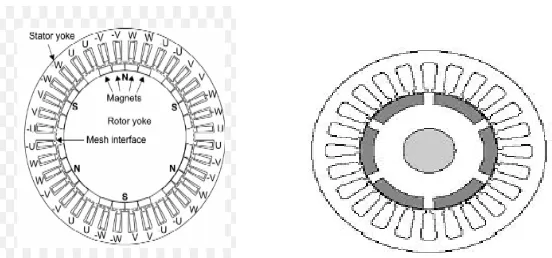
A permanent magnet synchronous motor (PMSM) is a motor that uses permanent magnets to produce the air gap magnetic field rather than using electromagnets. These motors have significant advantages, attracting the interest of researchers and industry for use in many applications.
PM motors are broadly classified by the direction of the field flux. The first field flux classification is radial field motor meaning that the flux is along the radius of the motor. The second is axial field motor meaning that the flux is perpendicular to the radius of the motor.
Radial field flux is most commonly used in motors and axial field flux have become a topic of interest for study and used in a few applications.
Permanent magnet motor radial field motors
In PM motors, the magnets can be placed in two different ways on the rotor.
Fig. 1. Surface magnet permanent motors Fig. 2. Interior permanent magnet motors
Each permanent magnet is mounted inside the rotor. It is not as common as the surface mounted type but it is a good candidate for high-speed operation. There is inductance variation for this type of rotor because the permanent magnet part is equivalent to air in the magnetic circuit calculation. These motors are considered to have saliency with q axis inductance greater than the d axis inductance
(Lq>Ld)
II. MATHEMATICALMODELLINGOFPMSM
In a permanent magnet synchronous motor the inductances vary as a function of rotor position i.e. the rotor angle. The emf of the PMSM is given by
= (1)
The position of the rotor is given by
= (2) Where is the electrical angle and is the mechanical angle
Fig. 3. Motor axis
Detailed modelling of PM motor drive system is required for proper simulation of the system. The d-q model has been developed on rotor reference frame as shown in figure 3. At any time t, the rotating rotor d-axis makes and angle θr with the fixed stator phase axis androtating stator mmf makes an angle α with the rotor d-axis. Stator mmf rotates at the same speed as that of the rotor.
= + (3)
= + (4) The rotor voltages and the stator voltages on the rotor reference frame is given by
=− − (5)
=− − (6) The total torque developed in the machine is given by
= − (7) is the torque of the prime mover.
is electromagnetic torque.
As the inductances keep changing with the rotor position and fluxes and currents are also dependent on the rotor position the parks and Clarks transformation are made use of to convert the linear time variant system to an linear time invariant system
= ( ) (8)
= ( ) (9)
= ( ) (10) Where is dependent on
=
⎣ ⎢ ⎢ ⎢
⎡ cos sin
cos( −2
3) sin( −
2
3)
cos( +2
3) sin( +
2
3) ⎦
⎥ ⎥ ⎥ ⎤
At steady state the rotor currents become constant and balanced sinusoidal
_ =
⎣ ⎢ ⎢ ⎢
⎡ cos cos −2
3 cos( +
2
3)
sin sin( −2
3) (sin +
2 3) ⎦ ⎥ ⎥ ⎥ ⎤ Where
= , = , = such that , , ≠0
Obtaining the mutual and the self-inductances due to coil on each of the rotor axis having the damper windings q, h, k,and g on direct and quadrature axis respectively.
Stator flux linkages given by,
− − − = − − − = − − =
Rotor flux linkage equations given by,
+ =
+ = 0
+ = 0
Obtaining the entire torque developed by the PMSM is given by,
= { − − − − − } (11)
= [ − ] (12)
Where,
= + (13)
= (14) Mutual inductance of the field and the a-axis is given by
III. MODELLINGOFBUILDINGSYSTEMPROTOTYPE(ELEVATOR)
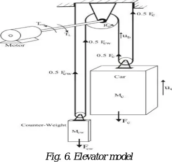
The elevator is used to transport people from one position to another in high rise buildings. The elevator is modeled considering all the realistic constraints.
Fig.4. Hooks modelFig. 5. Newton’s model
As rope exhibits two basic characteristics one is the stiffness and the other one is the elasticity with the damping. The Newton’s model is considered,
Fig. 6 shows the realistic model of the elevator with all the parameter values assumed to design the elevator model.
The torque equation of the elevator is given by,
= + ∗ + (15)
Where, is electromagnetic torque, is motor inertia and is the load torque. The load torque on the motor shaft running down the pulley is given by,
= ∗ + + (16)
Where, is pulley radius, is the force exerted by motor pulley
In order to obtain the overall working of the elevator the motion of the elevator has to be considered in two
directions. One direction is when the elevator is moving upwards and the other direction is when the elevator is moving downwards.
= [g*( − )+ ] (17)
Where, g is gravitational constant, is elevator car mass, is elevator counter weight. The belt is running at a speed of of the motor drive pulley.
= 2
Where, is motor speed.
=1
2
=1
2 ∗
Obtaining the power of car moving upward,
= ∗ ∗
Obtaining the pulling belt mechanical power,
=1
2 ∗ ∗
= ∗ *2
=
Equating the power of the moving car and mechanical belt and obtaining the force,
=1
2∗ ∗( − )
=1
2∗ ∗
= +
Assuming that the belt is flexible when moving upward and hence predicting that torque is unaffected due to these disturbances in the system.
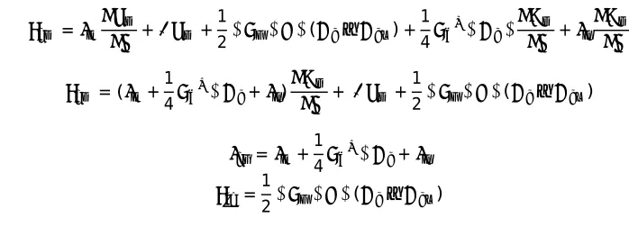
=1
2∗ ∗ ∗( − ) +
1
4 ∗ ∗ + +
The load torque when the elevator is moving downwards is given by,
( − )is load given to the elevator i.e. is the difference of mass of the car and the mass of the counter weight.
= + +1
2∗ ∗ ∗( − ) +
1
4 ∗ ∗ +
= ( +1
4 ∗ + ) + +
1
2∗ ∗ ∗( − )
Where,
= +1
4 ∗ +
=1
2∗ ∗ ∗( − )
IV.FIELDORIENTEDCONTROLOFPMSM
FOC control mainly involves converting the quantities from rotor reference frame to stationary reference frame and then converting the three phase to two phase orthogonal system.
Fig. 7.FOC Technique Fig. 8. FOC Transformations
Clarke’s transformations:
1. =
2. = ( + 2 )/√3
3. + + = 0
Park’s transformation:
1. = cos + sin
2. = cos − sin
Inverse Park’s transformation:
1. = cos − sin
2. = cos + sin
Inverse Clarke’s transformation:
1. =
2. = (− +√3 )/2
3. = (− − √3 )/2
V.SIMULATION AND RESULTS
A. Three phase voltage source inverter
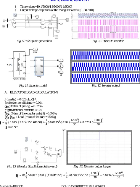
= 30
Time values= [0 1/5000/4 3/5000/4 1/5000]
Output voltage amplitude of the triangular wave= [0 -30 30 0]
Fig. 9.PWM pulse generation Fig. 10. Pulses to inverter
Fig. 11. Inverter model Fig. 12. Inverter output
A. ELEVATOR LOAD CALCULATIONS
J (inertia) = 0.0234 kg/ . B (friction co-efficient) = 0.004
(Radius of pulley) = 0.025m g (gravitational constant) = 9.8
(Mass of the counter weight) = 100 Kg
+Load (mass of the car) =150 Kg
=1
2∗0.025∗9.8∗(150−100) +
1
4∗0.0025 ∗150∗
1200
30 + 0.0234∗
1200 30
=4.8 Nm
Fig. 13. Elevator Simulink model(upward) Fig. 13. Elevator output torque
=−[1
2∗0.025∗9.8∗(150−100) +
1
4∗0.0025 ∗150∗
1200
30 + 0.0234∗
1200
=−4.8
Fig. 14.Elevator Simulink model(downward) Fig. 15.Elevator torque output
B. FIELD ORIENTED CONTROL CALCULATIONS
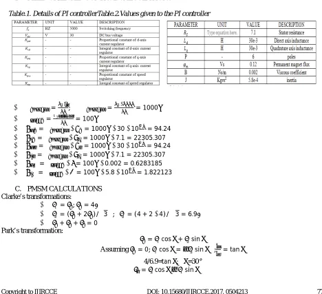
Table.1. Details of PI controllerTable.2.Values given to the PI controller
= ; = ∗ = 1000
= = 100
= ∗ = 1000 ∗30∗10 = 94.24
= ∗ = 1000 ∗7.1 = 22305.307
= ∗ = 1000 ∗30∗10 = 94.24
= ∗ = 1000 ∗7.1 = 22305.307
= ∗ = 100 ∗0.002 = 0.6283185
= ∗ = 100 ∗5.8∗10 = 1.822123
C. PMSM CALCULATIONS
Clarke’s transformations:
= ; = 4
= ( + 2 )/√3 ; = (4 + 2∗4)/ √3 = 6.9
+ + = 0
Park’s transformation:
= cos + sin
Assuming = 0; cos =− sin ; = tan
4/6.9=tan ; =30°
= 6.9 cos 30°−4 sin 30° =3.975A
Inverse Park’s transformation:
= cos − sin
= cos + sin
Inverse Clarke’s transformation:
=
= (− +√3 )/2
= (− − √3 )/2
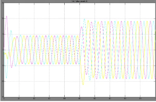
Fig. 16. Simulink model of the PMSM drive Fig. 17. Output torque, speed, current in q and d axis
Fig. 18. Stator three phase currents
VI.CONCLUSION
REFERENCES
[1] THOMAS M.JAHNS,GERALD B.KLIMAN,THOMAS W.NEUMANN “ Interior permanent-magnet synchronous motors for adjustable-speed drives”,IEEE transactions on industry applications,vol.IA-22, NO.4, July/August 1986
[2] THOMAS M JAHNS “ Flux weakening regime operation of an interior permanent magnet synchronous motor drive”, IEEE transactions on industry applications, vol.IA-23,NO.4,july/august 1987.
[3] TOMY SEBASTIAN GORDON R.SELMON “Operating limits of inverter driven permanent magnet motor drives”,IEEE transactions on industry applications, VOL.IA-23,NO.2, march/april,1987
[4] GILSU CHOI T.M.JAHNS “PM synchronous machine drive response to asymmetrical short –circuit faults”, IEEE transactions, 978-1-4799-5776-7/14
[5] GILSU CHOI THOMAS M. JAHNS “Investigation of key factors influencing the response of permanent magnet synchronous machines to three phase symmetrical short circuit faults” IEEE transactions on energy conversion, vol.31,no.4,December.2016
[6] R.T. UGALE B.N. CHAUDHARI “Rotor configurations for improved starting and synchronous performance of line start permanent magnet synchronous motor”IEEE transactions on industrial electronics,vol.64,no.1,January.2017