Scholarship at UWindsor
Scholarship at UWindsor
Electronic Theses and Dissertations Theses, Dissertations, and Major Papers
2013
Pathfinding by demand sensitive map abstraction
Pathfinding by demand sensitive map abstraction
Sourodeep Bhattacharjee University of Windsor
Follow this and additional works at: https://scholar.uwindsor.ca/etd
Recommended Citation Recommended Citation
Bhattacharjee, Sourodeep, "Pathfinding by demand sensitive map abstraction" (2013). Electronic Theses and Dissertations. 4720.
https://scholar.uwindsor.ca/etd/4720
Map Abstraction
By
Sourodeep Bhattacharjee
A Thesis Submitted to the Faculty of Graduate Studies
through School of Computer Science in Partial Fulfillment of
the Requirements for the Degree of Master of Science at the
University of Windsor
Windsor, Ontario, Canada 2012
c
by
SOURODEEP BHATTACHARJEE
APPROVED BY:
Dr. Myron Hlynka
External Reader
Department of Mathematics and Statistics
Dr. Dan Wu
Internal Reader School of Computer Science
Dr. Scott Goodwin
Advisor
School of Computer Science
Dr. Subir Bandyopadhyay
Chair of Defense School of Computer Science
I hereby certify that I am the sole author of this thesis and that no part of this thesis has been published or submitted for publication.
I certify that, to the best of my knowledge, my thesis does not infringe upon anyone’s copyright nor violate any proprietary rights and that any ideas, techniques, quotations, or any other material from the work of other people included in my thesis, published or otherwise, are fully acknowledged in accordance with the standard referencing practices. Furthermore, to the extent that I have included copyrighted material that surpasses the bounds of fair dealing within the meaning of the Canada Copyright Act, I certify that I have obtained a written permission from the copyright owner(s) to include such material(s) in my thesis and have included copies of such copyright clearances to my appendix.
In this thesis, we present a new algorithm: Demand Sensitive Map Abstraction (DSMA). DSMA is a special kind of hierarchical pathfind-ing algorithm in which we vary the granularity of abstraction of the high-level map based on pathfinding request demand associated with various regions in the high level map and the search time of the last path request. Additionally, the low level A* search is not restricted by the boundaries of the high level sectors. By dynamically varying the abstraction we are able to maintain a balance between path qual-ity and search time. We compare DSMA with two variations where the granularity of abstraction is constant; one of those contains maxi-mum granularity throughout (Dense HA*) and the other contains the minimum (Sparse HA*).
First of all, I would like to thank my supervisor - Dr. Scott Goodwin for being patient with me and for helping me nurture the idea of Demand Sensitive Map Abstraction; always commending the strong ideas while providing suggestions on improving the weak ones. I would also like to thank Dr. Richard Frost for showing how and where to find dependable research materials and how to extract essential information from lengthy papers quickly. I would like to thank my friend Mirna ˇSeˇci´c, for her recommendations on academic writing style and improving the graphics presented in this thesis. I am grateful to the committee members -Dr. Myron Hlynka and Dr. Dan Wu and the Chair Dr. Subir Bandyopadhyay for finding time from their busy schedules to attend my thesis proposal and defense.
Author’s Declaration of Originality . . . iii
Abstract . . . iv
Dedication . . . v
Acknowledgments . . . vi
List of Figures . . . ix
1 Introduction 1 1.1 Problem Domain . . . 1
1.2 Contribution . . . 1
1.3 Organization . . . 3
2 Hierarchical Pathfinding 4 2.1 Near Optimal Techniques . . . 5
2.1.1 Hierarchical A* . . . 5
2.1.2 Near Optimal Hierarchical A* . . . 7
2.1.3 Partial Pathfinding using Map Abstraction and Refine-ment . . . 11
2.1.4 Cooperative Pathfinding . . . 14
2.2 Improvements to Near Optimal Techniques . . . 18
2.2.1 Improving Collaborative Pathfinding using Map Ab-straction . . . 18
2.2.2 HPA* Enhancements . . . 20
3 Demand Sensitive Map Abstraction 23 3.1 Motivation . . . 23
3.2 Abstract Terrain Representation: Triangle Bin-trees . . . 25
3.3 Measuring Demand . . . 35
3.4 Composition and Decomposition Queues . . . 36
3.4.1 The Decomposition Queue . . . 36
3.4.2 The Composition Queue . . . 38
3.5 Operations . . . 42
3.5.1 The Decomposition Operation . . . 42
3.5.2 The Composition Operation . . . 47
4.2 Results and Discussion . . . 64
4.2.1 Path Quality . . . 64
4.2.2 Nodes Expanded . . . 68
4.2.3 Relative Time Consumption . . . 70
4.2.4 Comparison on Map . . . 71
5 Conclusion 72
6 Future Work 74
Glossary 75
Acronyms 76
References 77
1 Illustration of Pre-Processing step: Near Optimal HPA* . . . 8
2 Illustration of Intra/Inter Edges in Near Optimal HPA* . . . . 9
3 Illustration of QuickPath . . . 12
4 Experimental maps for WHCA*(w,a) and CPRA* . . . 19
5 Grid/Cell . . . 27
6 Illustration of Triangle Binary Tree . . . 28
7 Levels in Triangle Binary Tree . . . 30
8 Sample Game Map . . . 32
9 Sample Game Map with Grids . . . 33
10 Sample Game Map showing Hierarchical Clusters . . . 34
11 The Decomposition Queue . . . 36
12 Initial Decomposition Queue . . . 37
13 The Composition Queue . . . 38
14 Empty Composition Queue . . . 39
15 Initial Composition Queue . . . 40
16 Relative Demand Levels . . . 42
17 Decomposition . . . 44
18 The Decomposition Operation . . . 45
19 Relative Demand Levels . . . 48
20 Composition . . . 49
21 The Composition Operation . . . 50
22 Adjacent and Neighbor Triplets . . . 52
23 DSMA Map showing high level triplets and start and goal positions . . . 53
24 Two possible abstract paths . . . 54
25 Choosing the Adjacent Triplets . . . 55
26 Complete Abstract Path . . . 56
27 Actual Path . . . 57
28 An Alternate Case . . . 58
29 After Path Smoothing . . . 59
30 Sample Sparse HA* Map . . . 62
31 Sample Dense HA* Map . . . 63
32 Path Length Graph . . . 66
1
Introduction
1.1
Problem Domain
In this thesis we try to solve the problem of pathfinding in game maps.
Pathfinding is the problem of finding a route of desired quality from a given
start location to a given goal location in a game map. It consists of two
phases: path planning and path following; the latter encompasses the
traver-sal of planned path and dealing with unpredicted dynamic obstacles or other
mobile agents. In our thesis we restrict all our claims to path planning only.
We attempt to solve the problem of pathfinding in game maps using
hierarchical pathfinding techniques. Hierarchical pathfinding involves the use
of a high level abstract map created from the low level, actual, game map.
This is employed to overcome the exponential search time of A* search. We
assume that the map is known a priori and hence exploration is not necessary.
All our maps use grid worlds at their lowest level and the grids have octile
navigation which means a mobile agent can move north, south, east, west,
north-east, north-west, south-east and south-west.
1.2
Contribution
In this thesis we present a new algorithm which we call Demand Sensitive
Map Abstraction (DSMA). In this algorithm we vary the abstract map
dy-namically depending on the demand of pathfinding in a particular section
We claim that by varying the granularity of abstraction dynamically we
can make optimal use of resources (CPU time and memory space) to find a
suitable path, as opposed to keeping the granularity constant throughout the
game-play. There are set, industry standard, upper and lower bounds on the
time, that can be devoted to pathfinding when a game is being played which
is one millisecond (1 ms) to three milliseconds (3 ms). DSMA attempts to
keep the pathfinding time between these limits by varying the granularity
of abstraction, associated with either high demand or low demand regions,
depending on whether the last pathfinding time went above 3 ms (region is
split into two, finely grained, regions) or below 1 ms (two low demand regions
are coalesced to have a single, coarsely grained, region), respectively.
In order to prove our claim we compare DSMA to two other variations
where we do not vary the granularity of the abstract map. This gives us an
idea of the benefit we can get from dynamically varying the granularity of
abstraction. We measure path quality, pathfinding time and number of cells
explored to find a path. The experimental results support our claim, since
the performance metric curves of DSMA lie between the curves of the two
constant granularity variations.
Our work is significant because it is the first one to vary the
granular-ity of abstraction associated with specific regions instead of adding more
hierarchical levels to suit the resources available. So DSMA provides a new
philosophy of interpreting hierarchical pathfinding and opens up avenues for
1.3
Organization
This thesis contains four major sections: “Hierarchical Pathfinding” which
discusses the previous related work, “Demand Sensitive Map Abstraction” in
which we discuss our algorithm (DSMA) and explain why and how DSMA
works, “Experimental Analysis” where we discuss our experimental setup,
2
Hierarchical Pathfinding
The term “Hierarchical Pathfinding” was first penned in the paper
“Hierar-chical A*: Searching Abstraction Hierarchies Efficiently” (Holte et al., 1996),
which was the first paper that initiated this area of research. In large search
spaces with many obstacles and pathfinding units, the execution time of A*
search (Hart et al., 1968) becomes prohibitively large. To overcome this
prob-lem, Hierarchical pathfinding is employed. The process involves splitting up
the search space in regions and creating an abstract pathfinding map with
these abstract regions by placing an edge between connected regions. Each
region thus obtained can be further split into sub-regions. Each such
con-nection of regions form one level of hierarchy in the collection of pathfinding
maps. This process is carried out in a pre-processing step and all abstracted
regions are cached, along with the distance between them.
Later, during game play, when any game agent requests a path, the
algo-rithm begins searching for a path in the topmost abstract hierarchical map
by running A* search between regions. The path thus obtained is refined
subsequently by running A* search on lower level maps until the real game
map is reached. Collectively, the pre-processing and the on-line search is
called Hierarchical Pathfinding A*. This process ensures search for the path
2.1
Near Optimal Techniques
In this section we will discuss some of the first papers on Hierarchical
Pathfind-ing. The authors in these papers claim to have achieved results that are very
close to optimal or the desired least cost (edge weight) path. While all of
the papers discuss the idea of hierarchical pathfinding, their techniques are
different from each other and hence demand a discussion.
2.1.1 Hierarchical A*
The authors of the paper titled “Hierarchical A*” (Holte et al., 1996) claim
that this paper was the first one to address the problem of high execution
time of A* in large maps by applying Hierarchical Pathfinding techniques.
The motivation of this paper was to break Valtorta’s Barrier (Valtorta, 1983),
which is the number of nodes expanded when searching blindly. Valtorta’s
theorem (Valtorta, 1983) states that this barrier cannot be broken by
“em-bedding transformations” - abstracted state spaces. (Holte et al., 1996) is
different from the other papers discussed in this thesis, as it deals with puzzles
and not game world maps. Nonetheless it demands a discussion, since (Holte
et al., 1996) is the first paper to explore the idea of Hierarchical Pathfinding.
The idea proposed by the authors involved selecting a state (node in the
pathfinding graph) with maximum degree and grouping it together with its
neighbors within a certain distance (abstraction radius), and forming a single
node with them. The process was repeated until a level is created with only
When searching for a path in the lowest level, the algorithm proposed by
the authors, searched for a high level path in the abstract levels until the
highest level with a single state was reached. This algorithm was called
Naive Hierarchical A* (NHA*).
In their preliminary experiments the authors found that NHA* was
ex-panding more states than A*. They explained this observation by stating
that A* search using monotone heuristic will never expand the same state
twice. NHA*, on the other hand, expanded same states repeatedly in higher
levels for same start-goal pair in the base level. To overcome the problem they
introduced a technique they named h*-caching. The idea involved caching
h(s) values for states that have been expanded already and reusing these
val-ues in subsequent searches without expanding the state. Their experiment
showed that NHA* was expanding roughly the same number of states as A*.
This implied that Valtorta’s Barrier was not yet broken and more
enhance-ments were needed. The next improvement suggested by the authors relied
on the idea that for every state X for which h(X) is known, a path from
X to goal is also known. This precludes the necessity to expand X, if this
path is cached along with h(X). The authors state that “knowing a path of
length g(X) to X means knowing a path of length g(X) + h(X) to the goal”.
Instead of adding X to the open list, the goal state is added to it and the
search terminates when the goal is on top of the list. They call this technique
Optimal Path Caching. Thus NHA* with Optimal Path caching was able to
et al., 1996).
The paper concludes by mentioning two important future research areas:
firstly, the authors state that a better method is needed to vary the
granu-larity of abstraction and secondly, to find a better way to build abstracted
states automatically.
2.1.2 Near Optimal Hierarchical A*
The topic of Hierarchical Pathfinding was revived in the paper Near
Opti-mal Hierarchical Pathfinding (Botea et al., 2004). Their paper addressed
the problem of pathfinding on “large” maps where limited CPU and
mem-ory resources create severe bottlenecks. They achieved this by employing
hierarchical pathfinding techniques. (Botea et al., 2004) is very well
writ-ten and introduces many new ideas, algorithms and optimizations of those
algorithms.
The previous work referred to by the authors include (but are not
lim-ited to) (Rabin, 2000) and (Holte et al., 1996). The authors state that their
work is very similar to A* Aesthetic Optimizations (Rabin, 2000) in that
both employ hierarchical pathfinding by map abstraction. They differ in the
respect that the algorithms proposed by the authors support multiple levels
of hierarchy while the other supports only two. Another difference is that
in A* Aesthetic Optimizations, the optimal distances between two states are
computed on-line while in this paper the authors pre-compute and cache this
Hierarchi-cal A* (HA*) (Holte et al., 1996) in that both use hierarchiHierarchi-cal representation
of the search space for reducing search effort. However, the two papers are
different in the respect that Hierarchical Pathfinding A* (HPA*) proposed
by the authors uses abstraction to enhance the representation of the search
space while HA* is used for “automatically generating domain independent
heuristic state evaluations”.
The algorithm proposed by the authors consists of two phases: a
pre-processing step and an on-line search. The pre-pre-processing step defines a
topological abstraction of the map. The map is divided into rectangular
regions (“clusters”) as shown in the figure 1 below (Botea et al., 2004), p.24:
The authors then define a gateway between two clusters by identifying a
set of entrances connecting them, where an entrance is the longest
obstacle-free set of cells that lie in the border of two adjacent clusters. The transition
point (the point where an agent goes from one cluster to another) is the
midpoint of the entrance. The authors call this an inter-edge. For each pair
of such points inside a cluster, the authors link them by edges and name
them intra-edge. This forms a high level abstract graph. This is illustrated
in the figure below (Botea et al., 2004), p.24:
The next step consists of an on-line search. In this step the start and
goal nodes are inserted into the abstract graph and use A* search to find a
path from start to goal in the abstract graph. This gives an abstract path
which can be made concrete by mapping it to the low level graph and further
refining the path.
For their experiments, the authors used 120 maps from a game (Baldur’s
Gate from Bioware) varying in size from 50x50 to 320x320. For each map the
authors generated random start and goal states where a valid path between
the two existed. The authors state that A* is slightly better than HPA*
when the solution length is small (i.e., the search problem is easy). The
authors explain the difference in performance by stating that the overhead
of inserting start and goal states into the abstract graph and other such
techniques becomes an unnecessary expense when the map is mostly empty
or the path is possibly a straight line through the grid. However, given a
real game scenario with standard number of obstacles and mobile agents, the
authors claim that HPA* is up to 10 times faster than a highly optimized
A*.
With respect to their contribution the authors state that their method
of map abstraction is automatic and is independent of specific topology and
works well with both random and real maps as well as static or dynamic
environments. They also state that their technique is simple and easy to
2.1.3 Partial Pathfinding using Map Abstraction and Refinement
The next paper we are about to discuss, titled “Partial Pathfinding using Map
Abstraction and Refinement” (Sturtevant and Buro, 2005), is a significant
one. The reason for its significance lies with the fact that this paper is the
first one to explore the challenge of interleaving path planning with execution
in the hierarchical pathfinding framework. In this paper the authors propose
a set of algorithms they named - Path-Refinement A* (PRA*).
The authors refer to HPA* (Botea et al., 2004) as a related work. The
authors state that HPA* and PRA* is similar considering the fact that both
algorithms use hierarchical pathfinding. The two algorithms differ in the
respect that HPA* overlays an entire map with clusters/sectors and an
inter-connected set of such clusters form the high level graph, on the other hand
PRA*, instead of making a general abstraction of the entire map, studies the
map topology and groups together tiles (from the grid based low level map)
which are cliques forming one node and connects them with orphans.
The authors introduce their idea using a simple algorithm - QuickPath
and extend the same to PRA*, PRA*(∞) (one that finds complete paths)
and PRA*(k) (one that finds partial paths). The authors explain QuickPath
After building the abstraction hierarchy, all the nodes in the graph resolve
to a single high level node. To check if two nodes are connected, the algorithm
checks if they ever converge into the same parent within the abstraction
hierarchy. This provides a “quick check for path-ability” and can also find
plausible paths in the game world, by tracking the parents of the nodes,
without performing an extensive search, as claimed by the authors.
The PRA* proposed by the authors apply four enhancements to the
QuickPath algorithm. Firstly, the authors use a heuristic to make the search
more directed. Secondly, it allows path refinement in areas outside the
ab-stract path such as in corridors. Thirdly, it starts path-planning from the
bottom of the hierarchy instead of the top. Finally, it finds only partial
paths in the entire path planning step. Meaning the partial path thus found,
is executed/traveled by the agent before further planning. The QuickPath
algorithm ensures that planning and execution is interleaved. The authors
also propose two more variations: PRA*(∞) which is a version of PRA* in
which partial refinement is not allowed and PRA*(k) that refines k number
of nodes from the abstract path at a time. For experimentation, the authors
claim to have used 116 maps from Baldur’s gate and Warcraft 3 and scaled
them to size 512 X 512. The maps were represented as square tile grids with
octile relationship between tiles - an agent could move in eight directions
from any tile. They generated random start and goal pairs for each map.
They claim that PRA*(∞) has similar performance as HPA* and both are
PRA*(k) the authors state that the algorithm is “super-linear in the path
length”. They state that the paths derived from PRA*(k) are longer
com-pared to A* and PRA*(∞) but the algorithm proves to be faster than the
other two.
In conclusion, the authors claim that their paper was the first one to have
attempted partial pathfinding techniques and successfully interleaved
plan-ning with action. As future work, they plan to extend PRA* to incorporate
cooperative behavior.
2.1.4 Cooperative Pathfinding
The paper tilted Cooperative Pathfinding by Silver (Silver, 2005) addresses
the problem of multi-agent cooperative pathfinding where agents must
collab-orate with each other to find optimal paths to their destinations. Although
this paper is related to research on cooperative pathfinding, the reason we
are reviewing its contributions is that the algorithms suggested by the author
are inspired from and provide elegant extensions to HA*. We will see later
in our literature review how other scientists extended the work of Silver to
derive more general and robust Hierarchical Pathfinding algorithms.
The author refers to a general, industry standard, algorithm called Local
Repair A* (LRA*) which, the author claims, is often used in many video
games to tackle the problem of cooperative pathfinding. LRA* works by
re-planning an agent’s path, using the A* algorithm, when encountered with
by pointing out that in crowded situations, bottlenecks can take very long
time to get resolved. He also states that frequent re-planning in order to
avoid collisions creates “visually disturbing behavior that is perceived as
unintelligent”.
Silver proposes three novel algorithms in his paper : Cooperative A*
(CA*), Hierarchical Cooperative A* (HCA*) and Windowed Hierarchical
Cooperative A* (WHCA*). A brief description of the three algorithms are
as follows:
CA*: In this algorithm the path for each agent is calculated individually
in “three dimensional space-time” and a reservation table is maintained that
contains entries about the location of an agent (on the way to its goal) at
certain instances of time. An entry in the reservation table is avoided by
other agents when planning their routes. An additional “wait move” is also
incorporated in the table in which an agent waits for another agent to pass
before moving.
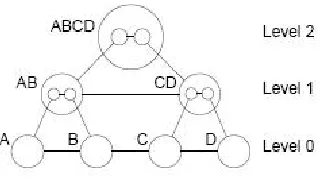
HCA*: This algorithm is inspired from HA* (Holte et al., 1996). However
the abstraction employed here simply consists of a high level map in which all
mobile obstacles, other than the current pathfinding agent, are non-existent.
The reservation table of CA* is used in tandem with the abstraction when
planning paths. Another feature of HCA* is that it uses Reverse Resumable
A* (RRA*) for calculating abstract distances between two locations. RRA*
works by running A* in reverse, from goal to start.
WHCA* calculates partial paths up to a certain depth. At regular intervals,
as the agent has followed a certain distance of the planned partial path, the
window depth is shifted forward (toward the goal) and a new partial path
is calculated. In order to guarantee that the agent is moving in the correct
direction, the path planning in the abstract map is performed up to the goal
(that is the complete path is calculated).
For the experiments, the author uses 10 randomly generated mazes. The
mazes were of size 32 x 32 and obstacles were strewn over 20% of the tiles.
The tiles were four-connected. Then random start and goal positions were
generated for a number of agents such that for no two agents, the start or
goal positions coincided. In the experiments, CA*, HCA*, WHCA* and
LRA* were compared in terms of success rate (agents being able to reach
goals within 100 turns), path length and cycle count ( an agent visiting an
already visited grid).
The author claims that as the map gets more crowded, LRA* begins to
struggle for a higher success rate. CA* and HCA* perform better than LRA*.
WHCA* performs the best in this regard, especially with a bigger window
size. For measuring path length, the author fixed the shortest distance as a
lower bound and claims that using LRA*, the path lengths are almost twice
the lower bound while CA* and HCA* finds paths that are only 20% above
the lower bound. With regard to the cycle count, the author states that
LRA* produces 10 times the number of cycles produced by the algorithms
In the concluding section, the author states that for “Simple
environ-ments”, LRA* is sufficient to find optimal paths. But in more complex
envi-ronments involving multiple moving obstacles, CA* and its family perform
2.2
Improvements to Near Optimal Techniques
2.2.1 Improving Collaborative Pathfinding using Map
Abstrac-tion
In the paper titled “Improving Collaborative Pathfinding using Map
Ab-straction” (Sturtevant and Buro, 2006), the authors address the problem of
cooperative pathfinding by combining partial pathfinding (Sturtevant and
Buro, 2005) with WHCA*(Silver, 2005) and cooperative pathfinding
tech-niques suggested by Silver (Silver, 2005) with PRA*(Sturtevant and Buro,
2005).
The authors refer to A* (Hart et al., 1968), WHCA*(Silver, 2005) and
their previous work PRA* (Sturtevant and Buro, 2005). While commenting
on the shortcomings of the previous work, the authors state that A* is
inad-equate for multi-agent pathfinding and WHCA* assumes some restrictions
such as four direction movements and constant speed of all units.
The authors propose two algorithms in (Sturtevant and Buro, 2006). The
first algorithm, WHCA*(w,a) is an extension of WHCA*. The new algorithm
accepts two parameters w (the window size) and a (the abstraction level used). This algorithm allows WHCA* to operate on higher levels of the
hi-erarchy instead of the base level. The second algorithm attempts to combine
WHCA* with PRA* yielding Cooperative Path-Refinement A* (CPRA*).
The algorithm uses PRA* at all levels of hierarchy other than the lowest
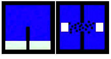
In order to compare the two new algorithms, the authors used the maps
shown below (Sturtevant and Buro, 2006), p.4. In these maps the darker
areas are not navigable, while the lighter are possible start and goal positions.
Mobile agents are made to move from a random location on the left side of
the maps to a random location on the right. The algorithms were compared
in terms of nodes expanded - initially (“during the first second”) and in
the subsequent seconds. Path quality was also compared by measuring the
maximum of total distance traveled by all agents.
From the results the authors obtained, it was deduced that WHCA*(w,a)
has a lower initial cost (expands less nodes in the first second) than CPRA*.
However in subsequent seconds CPRA* expands less nodes than WHCA*. In
terms of path quality, the authors state that the two algorithms have similar
performance.
Finally the authors conclude the paper by stating that if there are many
units in the game scenario and there are limitations in memory, then CPRA*
is a better choice than WHCA*(w,a). On the other hand if higher initial cost
is not a problem and there are no memory constraints, then WHCA*(w,a)
performs better. As future work, the authors plan to store information like
traffic congestion in the abstracted map, so as to avoid those routes when
planning. The authors also propose to dynamically vary the window size of
CPRA* according to the congestion level of the map.
2.2.2 HPA* Enhancements
In the paper titled “HPA* Enhancements” (Jansen and Buro, 2007), the
authors address the problem of optimal pathfinding using hierarchical
tech-niques. They do this by proposing three improvements to HPA*.
The previous work referred by the authors includes HPA* (Botea et al.,
2004), PRA* (Sturtevant and Buro, 2005) and Triangulation Refinement
A* (TRA*) (Demyen and Buro, 2006). While the authors do not find any
shortcoming of HPA*, they claim that the improvements suggested by them
The improvements suggested by the authors are as follows:
Faster Path Smoothing The authors state that in HPA* path smoothing
is performed to make them shorter and more optimal. The smoothing method
proposed by Botea et al. shoots imaginary straight lines in all eight directions
from each node n on the path. When a line reaches another node m further up
the path, the intermediate nodes between m and n are replaced by a straight
line and the algorithm continues with two positions before m on the new path.
The authors state that the computation involved is expensive, though the
path received is close to optimal. The authors address this issue by placing
a “bounding box” along the path to be refined. Place smaller bounding
boxes makes the smoothing process faster although the path received is less
optimal. The authors claim that the reduction is time has greater impact
than the slightly longer paths received on the overall quality of the process.
Using Dijkstra’s Algorithm To find paths between entrances of a
clus-ter, HPA* uses A* algorithm. The authors propose to use Dijkstra’s
algo-rithm instead since the worst case running time of A* is worse than the worst
case running time of Dijkstra’s single source shortest path algorithm.
Lazy Edge Weight Computation HPA*’s standard strategy to deal with
dynamic environments is to recompute entrances and edge weights of affected
clusters when changes occur in the game environment. The authors propose
authors state that in an optimistic situation the weights of some of the
un-necessary edges will never be calculated during the game play.
In order to test the theories, the authors use two sets of maps: the first
comprised of 116 real game maps from Baldur’s Gate and Warcraft III and
80 artificial maps; both were of size 512 x 512. The percentage of blocked
portion of the map was varied from 10 to 80. For each map, random start
and goal positions were chosen. The authors compare standard HPA* to
improved HPA* in terms of relative path length and time to find a path.
The experimental results they obtained suggested that pathfinding time
in-creases as the size of the bounding box is increased. They also find that
sub-optimality decreases as the size of the bounding box increases. They
also find that computing edge weights using Dijkstra’s algorithm takes far
less time than using A*. When testing the algorithms for lazy edge weight
computation, the authors claim to have found that using the lazy technique,
the abstract map is built very quickly since no expensive pre-computation of
edge weight is involved. They also state that the total time for calculating
edge weights was found to be less than the total time using the eager
ap-proach. The authors attribute this to the fact that some of edge weights are
never computed using the lazy approach.
In conclusion the authors state that the improvements to HPA* suggested
by them proves to be beneficial given the scope of the experiments performed.
They state that although preliminary results are promising, further research
3
Demand Sensitive Map Abstraction
3.1
Motivation
HPA* effectively solves the problem of pathfinding in large search spaces in a
reasonable amount of time. The technique, however, has its own limitations
which prevent it from being used in commercial games. The expensive
pre-caching of intra edges step saves a lot of time on scenarios where most of
the map is being used for pathfinding. On the other hand, the same feature
becomes an artifact when only a part of the map is traversable and
pre-caching intra edges of unused sectors of the map is entirely unnecessary
(Jansen and Buro, 2007). A corollary of the same situation occurs when the
map is dynamic and a change in Traversability in a portion of the map calls
for an expensive update of the abstract map. Another interesting observation
is that there is no scheme of varying the granularity of abstraction non-uniformly across the map in the HPA* paper or any of the literature that followed it -varying the granularity of abstraction, non-uniformly, (at the
single high level) depending on the last pathfinding time (time taken by the
A* search to find the previous path), is the central idea of our thesis.
The motivation for our thesis sprouts from the idea of tessellating terrain
using triangular bin-trees (Samet, 1990) (Duchaineau et al., 1997) and the
fact that it is reasonable to put a cap on the time required to find a path
from start to goal. An ideal time range to find an initial path would be
given the current technology standards. In the following paragraphs we will
emphasize the two ideas.
In the paper titled “ROAMing Terrain” (Duchaineau et al., 1997), the
authors use spatial data structures called triangle binary trees (bin-trees)
to dynamically vary the Level of Detail (LOD) in a map by using a grid of
triangles and splitting or merging them as needed to increase or decrease the
level of detail as needed, respectively. The dynamic LOD technique inspires
our thesis in that, we use the same data structure to create our abstract map
and dynamically vary the granularity of abstraction by joining or dis-joining
neighbor triangles. The reason for choosing triangle bin tress is that it was
found in (Demyen and Buro, 2006) that using triangles, instead of regular
quadrilaterals as in HPA*, to build the abstract map allows curved corners
and irregularly shaped obstacles to be incorporated in the map and make use
of extra space around them for pathfinding.
Now let us consider the second point in which we mentioned that it is
reasonable to keep the pathfinding time between 1-3 ms approximately. This
time does not include the path following or the execution step in which a game
agent travels the planned path. In the second chapter of the book (Dalmau,
2003), the author writes about real time game loop models; a comprehensive
discussion of the same is not in the scope of this thesis. The author defines
games as “time dependent interactive applications” consisting of a virtual
game world, a simulator to make the world seem real, a presentation layer
to interact with the virtual world.
To say games are time constrained, means a game must display
informa-tion at a constant speed which is usually above 25 frames per second (modern
games run 60 frames per second or more). More frames per second implies
less time available for real time simulators to modify the world to display
new states. Real time interactive applications such as games consist of three
tasks running simultaneously. First the current state of the virtual world
must be updated constantly, second the player must be able to interact with
the world and finally the result should be presented to the player using
visu-als and sounds. When information is displayed at 60 frames per second, the
simulator has only 16.67 ms (approximately) to modify the world (update
the world and render the result). The 16.67 ms in hand is to be spent
judi-ciously and hence only about 1-3 ms can be ideally devoted to pathfinding
according to Bulitko in (Bulitko et al., 2007).
In the next section, we will show how the above facts and conjectures are
woven together to derive Pathfinding by Demand Sensitive Map Abstraction
(DSMA).
3.2
Abstract Terrain Representation:
Triangle
Bin-trees
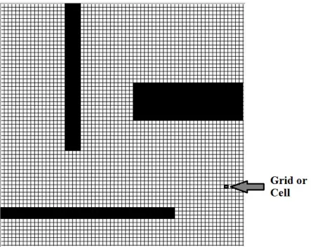
The current section gives an insight into Triangle Binary Trees. Please note
a minimum square unit of the game world (grid-based) that an agent or
obstacle can occupy (for our experiments each cell is 8 x 8 pixels) as shown
A triangle Binary tree (Lindstrom et al., 1996) (triangle bin-tree) is a
spatial data structure. Triangle bin-trees are binary trees with space
repre-sentational properties of Quad Trees. A triangle bin-tree is comprised solely
of right isosceles triangles and hence never develops Cracks or T-junctions.
Triangle bin-trees are mainly used for tessellating terrain (Duchaineau et al.,
1997).
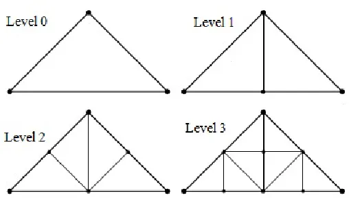
Let us consider the figure 6 above. The triangle bin-tree consists of a
triangle (I) and two possible children- a left child (III) and a right child (II).
When triangle I is decomposed, we obtain II and III. Similarly, when triangle
III is decomposed, triangles IV and V are produced. Conversely, it is also
possible to compose or merge two neighbor triangles to reduce granularity.
Such decomposing and composing can be continued until a suitable
granu-larity is reached for a given region or for the entire available area, uniformly
or non-uniformly. Hence, in our thesis we use triangle bin trees to
repre-sent hierarchical abstract maps so as to very the granularity of abstraction
dynamically according to demand.
It is necessary to keep track of all the neighbors of a particular triangle
so that cracks and T-junctions do not develop. In our implementation, we
store the triangles as Triplets of three grid coordinates in a hash table to
facilitate fast storage and retrieval. Henceforth, the term “triangle bin-tree”
and “triplet” will be used interchangeably, referring to any arbitrary
trian-gle in the abstract map. The neighbors are defined as triantrian-gles sharing two
common low level cells. For the high level A* search, triangles having one
common cell are considered as neighbors if other strongly connected
neigh-bors are not available. Every triangle has a level associated with it. When a
triangle at level n decomposes, the resulting child triangles are of level n+ 1.
Similarly when two triangles both at levelnmerge, the resulting triangles are
at level n−1. Any given configuration of states in a triangle binary tree can
The illustration of level change is given below:
The reason we are using triangle bin trees instead of quad trees as in
HPA*, is that in HPA* the hierarchical paths are pre-computed and cached;
while in our thesis we find hierarchical paths on-demand. Running A* search
on-demand in the hierarchal map using quad trees is, theoretically, an
ex-pensive process as there are more nodes to be processed (quads have more
entrances/sides than triangles). Moreover decomposing a quad will produce
four regular quads again making the hierarchical search expensive. On the
other hand triangles when decomposed produce two new triangles and each
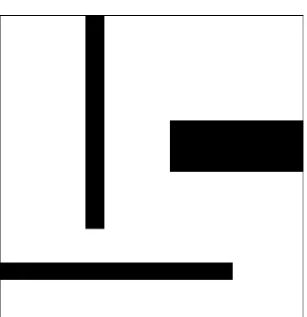
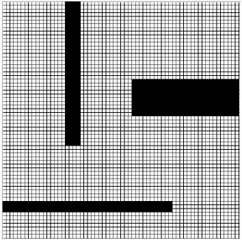
Let us consider a game map as shown in figure 8 above. The dark regions
represent obstacles and the white region is the navigable space. Our first
action is to lay grids on this map thereby getting the map as shown in figure
9 below. Each individual cell is 8 pixels by 8 pixels.
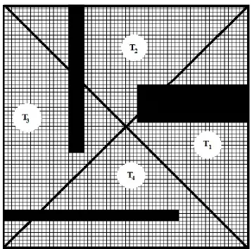
The initial hierarchal map is hard coded and will usually contain four
clusters as shown in figure 10 below, we have marked the four clusters as T1,
T2, T3, and T4 .
3.3
Measuring Demand
In our thesis, we vary the granularity of abstraction dynamically according
to the demand associated with triplets. Hence, in addition to level we add
another parameter- Demand, to triplets. A value associated with demand
represents how many times a triplet was explored in previous hierarchical A*
searches. Demand is increased by one, for triplets containing start and goal
nodes and for every triplet that gets expanded (explored) in hierarchical A*
search. We also decrease demand by one for every triplet that does not get
expanded in the high level A* search.
When the execution time of previous A* search rises above three
millisec-onds, we decompose the highest demand triplet (breaking ties arbitrarily)
thereby forcing the low level A* search to expand less nodes so that the total
search time is reduced. This step is expected to return less optimal path for
lower execution time.
Conversely, if the execution time of previous A* search falls below one
millisecond, we merge two of the lowest (collective) demand neighbor triplets
(breaking ties arbitrarily) since more time can be allocated to pathfinding.
Combining two low demand triplet forces the low level A* search to explore
more nodes. This is expected to result in more optimal paths at the expense
3.4
Composition and Decomposition Queues
Previously, we have discussed Triangle Bin Trees (Triplets) and how the
de-mand of a triplet is manipulated. In this section we will discuss the process
to keep track of high and low demand triplets and how we compose or
de-compose them when needed.
3.4.1 The Decomposition Queue
Figure 11: The Decomposition Queue
Initially this queue contains all triplets in the abstract map at level 0.
A visual representation is shown in figure 11. We assume that initially
all triplets in the abstract world (hard coded) are at their coarsest level;
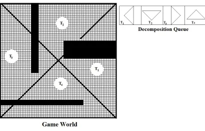
that is we do not decompose triplets at level 0. Figure 12 shows an initial
The interpretation of figure 12 is that the abstract map is composed of
four clusters T1, T2, T3 and T4 and each of the clusters can be further
decomposed to derive non-uniformly fine grained abstract map. If any of the
triplets is decomposed, each of the children will have half the demand of the
parent and level of the children will be one more then the one of the parents.
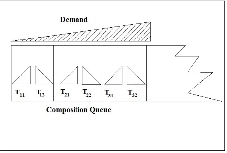
3.4.2 The Composition Queue
Figure 13: The Composition Queue
This queue contains pairs of triplets that can be composed or merged,
with the lowest demand pair in the front of the queue. Initially this queue
is empty. In our thesis and experiments we maintain a policy that triplets
at level 0 cannot be composed or merged. That is, the composition queue
of the initial map is empty. This policy can however be modified in future
However if one of the triplets (say T1) was decomposed in a previous
operation (into say T11 and T12), the composition queue would have one
entry as shown in figure 15 below.
The interpretation of the figure 15 is that triplets T11 and T12 can be
composed/merged later into the game-play to derive their parent triplet. If
T11 and T12 are composed the parents demand will be the collective (sum
of) demand of T11 and T12 and level of the parent will be one less than the
3.5
Operations
3.5.1 The Decomposition Operation
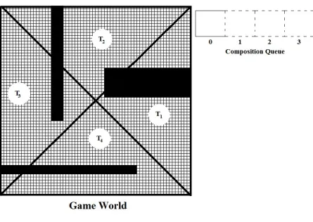
Consider the game map in figure 16; the dots represent the paths taken
by games agents. In other words, the dots are the foot prints of the agents.
As stated previously, we keep track of these footprints and use them to
dynamically vary the granularity of abstraction of the triplets. In addition to
that, we also keep track of the running time in A* search . If the last running
time of A* search went beyond of 3 milliseconds, we apply the decomposition
operation.
When the decomposition operation is applied, we extract the highest
demand triplet from the decomposition queue (T2 for the map shown above)
and we decompose it; thereby replacing T2 by it’s children T21 and T22 as
The way decomposition queue and composition queue is manipulated in
a decomposition operation is illustrated in figure 18 below.
Figure 18: The Decomposition Operation
Illustrated in figure 18 above is the decomposition process. We pop the
first triplet from QD, split the triplet as to form two isosceles triangles. Assign
the demands of T11 and T12 as half demand of T1 for both. From the triplet
that can be composed/merged and push it to QC. Additionally, it might
be possible to decompose T11 and T12 unless they have reached the finest
permissible granularity (say x). So, we preform the check for granularity and
push T11 and T12 to QD, if possible.
A simple algorithm for the decomposition operation is given below. TA
is the last running time of A* search and UTA is the Upper Threshold Time
decompo-sition queue while Qc is the compodecompo-sition queue.
Algorithm 1 Decomposition Algorithm
if T A≥U T A then
Decompose{t} Remove t from Qd Add t11 and t12 to Qd Add t11 and t12 pair to Qc
3.5.2 The Composition Operation
The reverse of the decomposition operation is the composition operation;
which we apply when the last running time of an A* search went below 1
millisecond. In this operation, we usually pick a triplet pair from the
compo-sition queue with lowest collective demand. Usually this is the first element
of the queue since we sort the composition in ascending order of collective
demand at regular intervals. For the game world depicted in figure 19, if the
last A* search time went below 1 millisecond, we would compose/merge T11
The procedure in which the two queues are handled in a composition
operation is illustrated in figure 21 below.
Figure 21: The Composition Operation
The illustration above shows the composition operation. A pair of triplets
is popped out of QD and their parent triplet is pushed into QD. Demand of
the parent is the combined demand of the child triangles. Since the demand
for triplets is varied in subsequent A* searches, it becomes necessary to
or-ganize QD and QC from time to time. Implying the content of the queues
are sorted according to demand in ascending order for QC and descending
save execution time.
Outlined below is a simple algorithm describing the steps involved in
composition operation. TA is the last running time of A* search, LTA is
the Lower Threshold Time Limit for A* search which is 1 millisecond in our
thesis. We assume that at the front for the composition queue is an arbitrary
triplet pair ti1 and ti2. That is the pair has the lowest collective demand
compared to all other triplet pairs.
Algorithm 2 Composition Algorithm
if T A≤LT A then
Compose{ti1 ,ti2 } { This step results in parent triplet ti }
Remove ti1 and ti2 from Qd Add ti to Qd
Remove ti1 and ti2 pair from Qc
3.6
Pathfinding using DSMA
Triplet Relationships In this section we will discuss how DSMA finds
path given a certain high level map. Two triplets in DSMA can have two
kinds of relationships- they can be adjacent to each other or they can be
neighbors. Adjacent triplets are those that have a side (or part of it) in
common. Neighbor triplets have only one vertex (cell) in common. Hence
all adjacent triplets are neighbors but not all neighbors are adjacent to each
other. All neighbors are considered in the high level search as well. The
relationships are demonstrated in the figure 22 below:
Figure 22: Adjacent and Neighbor Triplets
In I above all the neighbors are a,b,c and d while the adjacent triplets are
(a,b), (b,c),(c,d) and (d,a). In figure II above both c11 and c12 are adjacent
Pathfinding Now let us consider the map in figure 23 below with the start
and goal positions marked as S and G, respectively:
As we can see above the start and the goal cells are ambiguously placed
such that their centers lie on the border of the triplets. Since we use
IsVis-ible() method in GraphicsPath in C#, the method resolves such conflicts
arbitrarily. One could possibly, as future work, break the tie by placing the
grids in a triplet whose centroid is closest to the center of the cell. With the
IsVisible() method we have used, the high level A* search can possibly take
two directions as shown in figure 24 below:
Let us proceed with case I above because it poses a new challenge which
we will explore. The high level A* search considers an abstract path from
start to the centroid of t1 as shown in the dashed line below.
The high level A* search does not consider obstacles, unless a triplet is
over 90% full or an obstacle covers the centroid. If it is more than 90% full,
a penalty is added to the triplet’s f-value during high level A* search. If an
obstacle is covering a centroid, the low level A* search attempts to connect
the present way-point to the next way-point (centroid), after skipping the
centroid being covered by an obstacle.
The high level A* search considers two of its adjacent triplets shown in
bold lines in figure 25 above and selects t2 as it has a lower f-value. The
tentative abstract path from t1 to t2 is shown in the dashed line above.
Now, let us assume that the goal is in t3. The only adjacent triplet to t2
is t3 and t3 contains the goal. Hence the high level search is successful and
the complete abstract path is shown in figure 26 below:
Thus the high level A* search has discovered way-points which the low
level A* search must now connect to get the actual path. We are assuming
that the abstract path is optimal since we have used A* search and it is to
be noted that the diagram above is not to scale.The challenge of crossing the
obstacle, we mentioned above has been resolved by the low level A* search,
as shown in figure 27 below:
Another very important property of DSMA evident from the above is
that the low level search is not restricted to the boundaries of the high
level triplets. This is a departure from conventional hierarchical pathfinding
techniques where the low level A* search is restricted to the boundaries of
the high level clusters, as mentioned in the introductory paragraph of section
2.
An Alternate Case: Let us consider a case in which the goal was found
(arbitrarily) to be in t4 instead of t3. The resulting high level abstract path
and actual path is shown in figure 28 below as I and II respectively:
The resulting path has a detour via the centroid of t4. There are two
solutions to resolve the problem, assuming that A* does not find the path
via t5 and t4 to be more optimal. One has already been mentioned above
- to resolve the conflict by Euclidean distance from the centroid. The other
solution is expensive but widely used to achieve better path quality- path
smoothing and refinement techniques (Botea et al., 2004). The techniques
were used in HPA* to remove undesirable detours. Once path smoothing is
applied, we can expect to receive as path as shown below:
4
Experimental Analysis
4.1
The Setup
In this section we perform a set of experiments. This section describes the
experimental setup. All experiments are inspired from (Jansen and Buro,
2007) and (Sturtevant and Buro, 2005).
Maps and Obstacles We use ten different maps inspired from commercial
RTS games. Each of the maps are scaled to three different pixel sizes: 256
by 256, 512 by 512 and 1024 by 1024. This gives us 30 different maps.
All maps are grid worlds with octile navigational freedom. We conduct all
experiments with one agent only, as our claims and experiments encompass
the domain of path planning only and not the nuances of path following.
In addition to hard coded obstacles in the maps,we also introduce random
obstacles into the map (between calls to the respective algorithms; that is
without modifying the map when a certain instance of path planning is in
progress). The random obstacles are varied in density from 20% to 40%;
always ensuring that the start and goal points are connected. That is, a
path exists between the start goal points, for the algorithms to discover. We
ensure this by running A* search first and if the search fails we discard the
start-goal pair. All obstacles are made to fit to cells, that is, an obstacle
Procedure In order to compare the algorithms we generate 500 random
start and goal locations for every map. We compare DSMA to two versions of
a generic hierarchical A* search. The first version has a sparse and constant
(single level) abstract map, containing eight triplets. We call this algorithm
sparse HA*. The second version has a denser and constant (single level)
abstract map, containing 64 triplets.We call this algorithm dense HA*. The
sparse map has 8 triplets beacause that is the minimum number of triplets
DSMA is allowed to have and the dense has 64 because that was maximum
number of triplets used in HPA* experiments and that is the maximum
number of triplets we allow DSMA to create. It is to be noted that we are
using some of the experimental standards of HPA* and not comparing DSMA
to HPA*. By sparse or dense we are referring to the number of clusters in
The clusters are regular and hard coded. We are comparing DSMA to
sparse and dense HA* to see if we can benefit from dynamically varying the
granularity of abstraction, as opposed to having a static abstract map. We
also compare DSMA to a naive A* search, to get a theoretical comparison
to HPA*. The lower level A* search for all algorithms uses a hybrid
heuris-tic (Chebyshev distance) for diagonal movements and Manhattan distance
for straight line moves, whereas the high level A* search for all algorithms
uses Euclidean distance as a heuristic. All heuristics mentioned above are
consistent and hence admissible as well.
Performance Metrics and Presentation of Results While carrying
out the experiments we record the number of nodes expanded by the high
level A* and the low level A* search combined, the time taken to find a
path (including the overhead time for sorting the queues and
decomposi-tion/composition) and the length of path for each algorithm for the same
map and same start-goal points. We do not use any form of path
smooth-ing or refinement to keep our focus strictly on the behaviour of DSMA. We
present highlights of the raw data in graphs in the next section.
4.2
Results and Discussion
4.2.1 Path Quality
Firstly, let us consider the graph below depicting relative path lengths of
in the x axis. This graph is taken from the maps of size 256 by 256 pixels.
The points are average path lengths returned for a given A* path length.
The tables are sorted in ascending order by A* path lengths, before the
averages are determined. So it must be noted that the points plotted are not
in sequential time.
We observe that the DSMA algorithm balances the path length according
to the time taken by the respective last A* search. The DSMA graph has
sharp hills and valleys due to the reason that the map is small and the random
start-goal generator very often produces two close points. This results in the
search time being less than 1ms and subsequently a composition. A sequence
of such frequent compositions raises the search time again. So, it can be said
that DSMA responds well to the dynamic changes. The sensitivity of DSMA
The graph below is for maps of size 1024 by 1024 pixels. The graph for
map size 512 by 512 is similar and hence is not shown to avoid redundancy.
This graph is smoother than the one above since the map size is large and
the probability of the randomly generated start-goal points being far away
is high. So we get a wide range of values from the path length of A* search
and hence the number of corresponding values being averaged is small with
low standard deviation; while the number of points being plotted is high.
4.2.2 Nodes Expanded
The graph below shows the relative number of nodes expanded by Dense
HA*, DSMA and Sparse HA* against the optimal path length for map size
1024 by 1024 pixels. It is evident that DSMA can keep the nodes expanded
between those given by the dense and sparse configurations. Another
corol-lary observation is that depending on the situation, DSMA can behave like
the Dense HA* or Sparse HA* there by striking a balance between search
time and path quality. The graphs for 256 by 256 and 512 by 512 have similar
4.2.3 Relative Time Consumption
The bar chart below shows the relative time consumption of Dense HA*,
DSMA, Sparse HA* and A*. We can say that for smaller maps Dense HA*
, DSMA and Sparse HA* have very similar performance, so using DSMA
is not very advantageous. However as the map size grows, the differences
increase and DSMA is a better choice especially when the map is dynamic.
The results presented below are to give a general idea of the time differences
and have high standard deviations especially for DSMA as it keeps adjusting
the time.
4.2.4 Comparison on Map
The explanation of the results is provided in the self-explanatory diagram
below where the start and goal are marked as S and G. The dots represent the closed list of the low level A* search and the circles are waypoints provided
by the high level search. The line connecting the start and goal represents
the final path.
5
Conclusion
In this thesis we presented a new hierarchical pathfinding algorithm- Demand
Sensitive Map abstraction in which we vary the granularity of abstraction
dynamically depending on the pathfinding demand associated with various
regions of the high level map and the last pathfinding time. DSMA is an
alternative to the HPA* (and other related work), as HPA* pre-caches all
intra-edges and DSMA does not have intra or inter edges. Instead DSMA uses
a hybrid abstract edge that is computed on the fly. Moreover, the low level
A* search in DSMA is not restricted to the boundaries of high level triplets
and this makes DSMA a special kind of hierarchical pathfinding algorithm.
DSMA is compared it to two cases: a highly detailed abstract map and
a low detail abstract map. The results we derived are promising as DSMA
is successful in balancing the path quality and search time and continuously
evolves the abstract map to keep the balance. The highly detailed abstract
map used in Dense HA* has similar configuration (number of high level
clusters) as those used in experiments for HPA* and we found that if resources
permit, DSMA can perform as efficiently (time-saving) as the dense HA*. On
the other hand, if the search time permits, DSMA can be made to resolve
into sparse HA* (approximately similar performance to naive A* search) .
Moreover we do not pre-cache paths, so DSMA can be applied to dynamic
maps without any modification.
pixels or higher to gain maximum advantage from varying the abstractions
6
Future Work
As future work, we plan to implement forced composition and
decomposi-tion. A forced composition is one where the two triplets being composed
do not come from the same parent and a forced decomposition is one in
which we have to perform an additional decomposition in order to
decom-pose a particular triplet or diamond. It would be interesting to experiment
with different values of upper and lower threshold values of search time as
well. Similarly it is also possible to experiment with different maximum and
Glossary
Chebyshev distance In the context of A* search, Chebyshev distance heuris-tic returns a value of estimated path cost to goal such that a diagonal move (North-East, North-West, South-East or South-West) is different from a straight line movement (North, South, East or West). The fac-tor by which the two moves differ can be freely modified as desired. 65
Clique A clique in an undirected graph is a subset of its vertices such that every two vertices in the subset are connected by an edge. 11
Cooperative Pathfinding Cooperative pathfinding refers to a multi agent path planning problem in which agents must collaborate with each other to find optimal paths to their destinations, given complete infor-mation about the paths of each other. 14
Cracks These are defects resulting from polygonal mesh irregularities. The name comes from the discontinuity in terrain arising due to mis-alignment of mesh vertices. 28
Level of Detail (LOD) A term related to computer graphics, controlling level of detail involves diminishing the detail of an object representation as it moves away from the camera or according to other reference points such as object importance, eye-space speed or position. 24
Manhattan distance In the context of A* search and pathfinding, Man-hattan Distance is a heuristic that returns a path cost estimate to the goal equal to the sum of the required displacement horizontally and vertically. 65
Orphan A node in a graph that can be reached by a single operator. 11
T-junctions These are caused by irregular intervals between mesh ver-tices.The phenomenon is described as presence of a vertex in higher level that is not connected to any vertex in the lower levels. 28
Traversability Every position in a given map is associated with a value. This value indicates the traversability of that position. A game agent can access that position until the value reaches a certain threshold, beyond which the position is said to be untraversable or blocked. 23
Acronyms
CA* Cooperative A*. 15–17
CPRA* Cooperative Path-Refinement A*. 18, 20
DSMA Demand Sensitive Map Abstraction. 25, 62, 65
HA* Hierarchical A*. 7, 8, 14, 15, 62, 65
HCA* Hierarchical Cooperative A*. 15, 16
HPA* Hierarchical Pathfinding A*. 8, 10, 11, 13, 20–22, 31, 62, 65
LRA* Local Repair A*. 14, 16, 17
NHA* Naive Hierarchical A*. 6
PRA* Path-Refinement A*. 11, 13, 14, 18, 20
RRA* Reverse Resumable A*. 15
TRA* Triangulation Refinement A*. 20
References
Botea, A., M¨uller, M., and Schaeffer, J. 2004. Near Optimal
Hier-archical Path-Finding. Journal of Game Development 1, 1, 7–28.
Bulitko, V., Sturtevant, N. R., Lu, J., and Yau, T. 2007. Graph
abstraction in real-time heuristic search. J. Artif. Intell. Res. (JAIR) 30, 51–100.
Dalmau, D. S. C. 2003. Core Techniques and Algorithms in Game
Pro-gramming. New Riders Publishing.
Demyen, D. and Buro, M. 2006. Efficient triangulation-based
pathfind-ing. In AAAI.
Duchaineau, M., Wolinsky, M., Sigeti, D. E., Miller, M. C., Aldrich, C., and Mineev-Weinstein, M. B.1997. Roaming terrain:
real-time optimally adapting meshes. InProceedings of the 8th conference on Visualization ’97. IEEE Computer Society Press, 81–88.
Hart, P. E., Nilsson, N. J., and Raphel, B. 1968. A formal basis for
the heuristic determination of minimum cost paths. InIEEE transactions on Systems Science and Cybernetics. 100–107.
Holte, R. C.,Perez, M. B.,Zimmer, R. M.,and MacDonald, A. J.
1996. Hierarchical A*: searching abstraction hierarchies efficiently. In
Proceedings of the thirteenth national conference on Artificial intelligence - Volume 1. AAAI Press, 530–535.
Jansen, M. R. and Buro, M.2007. HPA*enhancements. InAIIDE. 84–87.
Lindstrom, P.,Koller, D.,Ribarsky, W.,Hodges, L. F.,Faust, N., and Turner, G. A.1996. Real-time, continuous level of detail rendering
of height fields. InProceedings of the 23rd annual conference on Computer graphics and interactive techniques. SIGGRAPH ’96. ACM, 109–118.
Rabin, S.2000. A* Aesthetic Optimizations. InGame Programming Gems.
Samet, H.1990.Applications of spatial data structures - computer graphics,
image processing, and GIS. Addison-Wesley.
Silver, D.2005. Cooperative Pathfinding. InGame AI Programming
Wis-dom 3. Charles River.
Sturtevant, N. R. and Buro, M. 2005. Partial pathfinding using map
abstraction and refinement. InProceedings of the 20th national conference on Artificial intelligence - Volume 3. AAAI Press, 1392–1397.
Sturtevant, N. R. and Buro, M. 2006. Improving collaborative
pathfinding using map abstraction. In AIIDE. 80–85.
Valtorta, M. 1983. A result on the computational complexity of heuristic
Vita Auctoris
NAME: Sourodeep Bhattacharjee
PLACE OF BIRTH: Howrah, India.
YEAR OF BIRTH: 1987
EDUCATION:
2006-2010
Bachelor of Technology
Computer Science and Engineering Asansol Engineering College