Structural Complexity of Manufacturing Systems Layout

(1)

University of Windsor University of Windsor

Scholarship at UWindsor

Electronic Theses and Dissertations Theses, Dissertations, and Major Papers

2012

Structural Complexity of Manufacturing Systems Layout

Valeria Betzabe Espinoza Vega

University of Windsor

Follow this and additional works at: https://scholar.uwindsor.ca/etd

Recommended Citation Recommended Citation

Espinoza Vega, Valeria Betzabe, "Structural Complexity of Manufacturing Systems Layout" (2012). Electronic Theses and Dissertations. 5351.

https://scholar.uwindsor.ca/etd/5351

This online database contains the full-text of PhD dissertations and Masters’ theses of University of Windsor students from 1954 forward. These documents are made available for personal study and research purposes only, in accordance with the Canadian Copyright Act and the Creative Commons license—CC BY-NC-ND (Attribution, Non-Commercial, No Derivative Works). Under this license, works must always be attributed to the copyright holder (original author), cannot be used for any commercial purposes, and may not be altered. Any other use would require the permission of the copyright holder. Students may inquire about withdrawing their dissertation and/or thesis from this database. For additional inquiries, please contact the repository administrator via email

(2)

Structural Complexity of Manufacturing Systems Layout

by

Valeria Betzabe Espinoza Vega

A Thesis

Submitted to the Faculty of Graduate Studies

through Industrial and Manufacturing Systems Engineering in Partial Fulfillment of the Requirements for

the Degree of Master of Applied Science at the University of Windsor

Windsor, Ontario, Canada

(3)

Structural Complexity of Manufacturing Systems Layout

by

Valeria Espinoza

APPROVED BY:

______________________________________________ Dr. Darren Stanley

Faculty of Education

______________________________________________ Dr. Ahmed Azab

Dept. of Industrial and Manufacturing Systems Engineering

______________________________________________ Dr. Hoda ElMaraghy, Advisor

Dept. of Industrial and Manufacturing Systems Engineering

______________________________________________ Dr. Waguih ElMaraghy, Chair of Defense

(4)

iii

DECLARATION OF CO-AUTHORSHIP/PREVIOUS PUBLICATION

This thesis includes one original paper that has been previously submitted for publication

in a peer reviewed conference proceedings, as follows:

Thesis Chapter Publication Title/Full Citation Publication Status

Chapter 3

V. Espinoza, H. ElMaraghy, T.

AlGeddawy, S.Samy (2011).

“‟Assessing the Structural Complexity of Manufacturing Systems Layout”,

In: 4th CIRP Conference on Assembly

Technologies and Systems.

Submitted

I certify that, to the best of my knowledge, my thesis does not infringe upon anyone‟s

copyright nor violate any proprietary rights and that any ideas, techniques, quotations, or

any other material from the work of other people included in my thesis, published or

otherwise, are fully acknowledged in accordance with the standard referencing practices.

Furthermore, to the extent that I have included copyrighted material that surpasses the

bounds of fair dealing within the meaning of the Canada Copyright Act, I certify that I

have obtained a written permission from the copyright owner(s) to include such

material(s) in my thesis and have included copies of such copyright clearances to my

appendix.

I declare that this is a true copy of my thesis, including any final revisions, as approved

by my thesis committee and the Graduate Studies Office, and that this thesis has not been

(5)

iv ABSTRACT

The layout of a manufacturing facility/system not only shapes material flow pattern and

influence transportation cost, but also affects the decision making process on the shop

floor. The layout of manufacturing systems determines the information content of its

structural complexity inherent in the layout by virtue of its configuration design.

This thesis proposes a methodology which converts the physical system layout to a

graphical representation to produce measurable complexity indices. The elements to

represent the physical layout are the number of places where decisions are made and

relationships within the layout. The structural characteristics of the layout include

density, paths, cycles, decision points, redundancy distribution and magnitude, which are

captured by the complexity indices. The indices are directly determined by the

information content, and the layout complexity index (LCI) combines those individual

indices representing the structural complexity of the layout. The LCI is insensitive to the

sequence of the complexity index values, which is its main advantage. The methodology

is applied to six manufacturing systems layouts. Two layouts from the literature were

used for comparison purposes since their complexity was previously assessed. The

developed method is used to design the least complex layouts and to compare alternative

(6)

v DEDICATION

This thesis is dedicated to all members of my family, each one has taught me

something very special. Especially to my parents Sergio Espinoza and Laura Vega who I

(7)

vi

ACKNOWLEDGEMENTS

I would like to extend my sincerest thanks to my supervisor, Dr. Hoda

ElMaraghy, for giving me the opportunity to collaborate in her research group and for her

knowledge, guidance, suggestions, and encouragement provided during my Master‟s

studies.

Special thanks to my committee members Dr. Ahmed Azab and Dr. Darren

Stanley for their input and valuable advice given. Special thanks to Dr. Waguih

ElMaraghy for his knowledge through the graduate courses and to Dr. Tarek AlGeddawy

and Dr. Sameh Badreous for their valuable expertise and discussion about this thesis.

A warm thanks to Erica Lyons for her extremely kind support through this

process.

My best and sincere thanks to Waldo Perez for all his support, guidance, patience,

encouragement, and love. None of this would be possible without you.

Lastly, special thanks for the financial support provided by the Secretary of Public

(8)

vii

TABLE OF CONTENTS

DECLARATION OF CO-AUTHORSHIP/PREVIOUS PUBLICATION ... iii

ABSTRACT ... iv

DEDICATION ...v

ACKNOWLEDGEMENTS ... vi

LIST OF TABLES ... xi

LIST OF FIGURES ... xiii

CHAPTER I. INTRODUCTION 1.1 Motivation ...1

1.2 Complexity in Manufacturing Systems Layout ...2

1.3 Hypothesis ...4

1.4 Research Questions ...4

1.5 Objectives ...5

1.6 Scope of the Research ...5

1.7 Structure of the Thesis ...6

II. REVIEW OF LITERATURE 2.1 Manufacturing Systems ...8

2.2 Layout Configuration ...10

2.3 Manufacturing System Configurations ...12

2.4System Performance Approach ...16

2.5 Summary ...19

2.6 Complexity ...19

2.7 Approaches to Measuring Complexity in Manufacturing ...22

2.7.1 Entropy/ Information Approach ...22

2.7.2 Complexity in Axiomatic Design...25

2.7.3 Heuristic Approach ...29

2.7.4 Hybrid Approach ...30

2.8 Complexity in Other Fields of Engineering ...33

2.8.1 Complexity in Product Development ...33

2.8.2 Complexity in Computer Science ...34

(9)

viii

2.9 Summary of the Literature Review on Complexity in Manufacturing ....38

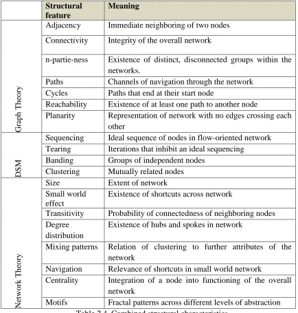
2.10 Graphs ...40

2.11 Network Theory ...42

III. ASSESSING THE STRUCTURAL COMPLEXITY OF A MANUFACTURING SYSTEM LAYOUT 3.1 Introduction ...44

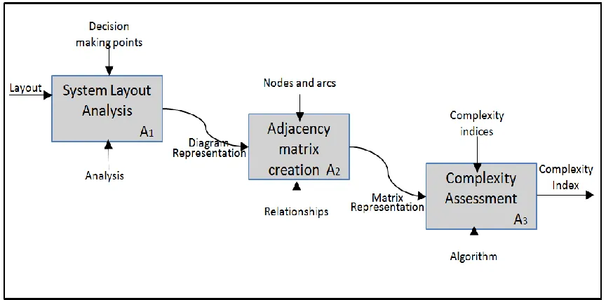
3.2 System Layout Analysis ...45

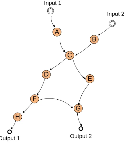
3.3 Diagram Representation ...45

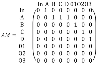
3.4 Adjacency Matrix Creation ...46

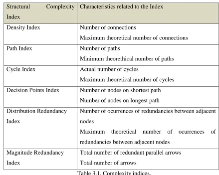
3.5 Complexity Indices ...47

3.5.1 Density Index ...49

3.5.2 Path Index ...50

3.5.3 Cycle Index ...52

3.5.4 Decision Points Index ...54

3.5.5 Redundancy Distribution Index ...56

3.5.6 Redundancy Magnitude Index ...57

3.6 Layout Complexity Assesment ...59

3.6.1 Average Value ...59

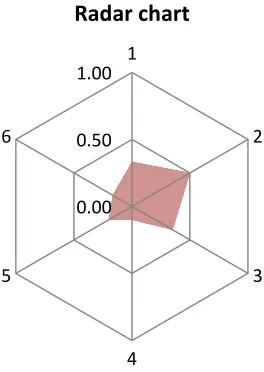
3.6.2 Radar Chart ...60

3.6.3 Vector Method ...62

3.6.4 Summary of the Techniques...62

IV. APPLICATIONS OF THE METHODOLOGY 4.1 ABS Plant Layout ...64

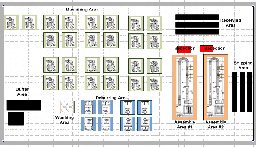
4.1.1 System Layout Analysis ...64

4.1.2 Diagram Representation ...65

4.1.3 Adjacency Matrix for ABS Plant Layout ...66

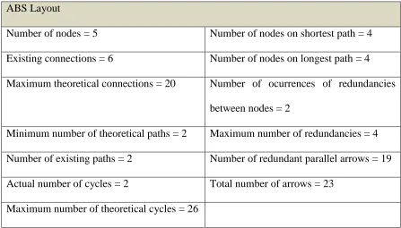
4.1.4 Complexity Indices ...67

4.1.5 System Layout Complexity Assessment ...68

4.1.5.1 Average Complexity Index ...68

4.1.5.2 Complexity Index Using the Radar Chart ...68

4.2 ABS Modified Layout ...69

4.2.3 Adjacency Matrix Creation ...71

(10)

ix

4.3 Modular Layout ...74

4.4 Hybrid Serial/Parellel System Layout ...79

4. 5 Automobile Engine Piston Assembly Plant Layout ...84

4.6 American Axle & Manufacturing (AAM) Plant Layout ...89

4.6.5.2 Complexity Index Using the Radar chart...94

4.7 Independence of the Complexity Indices ...95

(11)

x

5.2 Sensitivity of the Radar Chart ...100

5.3 Layout Complexity Index (LCI) ...103

5.3 Layout Complexity Index for System Layouts ...106

5.4 Analysis and Discussion ...108

5.4.1 Discussion From Previous Assessment ...108

5.4.2 Discussion From the Case Study Results ...109

5.5 Hypothesis and Research Questions ...109

5.6 Conclusions ...111

5.7 Contributions to Knowledge ...112

APPENDICES ...113

Appendix A ...113

REFERENCES ...116

(12)

xi

LIST OF TABLES

Table 2.1. Characteristics of dedicated, RMS and FMS. ... 9

Table 2.2. Comparing parallel lines and RMS configuration. ... 15

Table 2.3. Matrix of literature review. ... 37

Table 2.4. Combined structural characteristics. ... 43

Table 3.1. Complexity indices. ... 48

Table 3.2. Comparison of Complexity Index Calculation Techniques. ... 63

Table 4.1. Factors related to indices for ABS layout. ... 67

Table 4.2. Complexity Indices of the ABS layout. ... 68

Table 4.3. Factors related to indices of the ABS modified layout. ... 72

Table 4.4. Complexity indices of the ABS modified layout. ... 73

Table 4.5. Factors related to indices for the modular layout. ... 77

Table 4.6. Complexity indices of the modular layout. ... 78

Table 4.7. Factors related to indices of the hybrid layout. ... 82

Table 4.8. Complexity indices of the hybrid layout... 82

Table 4.9. Factors related to indices for the assembly engine layout. ... 87

Table 4.10. Complexity indices of the assembly engine layout. ... 87

Table 4.11. Factors related to indices for the AAM layout. ... 93

Table 4.12. Complexity Indices of the AAM layout. ... 93

Table 4.13. Complexity indices for six layouts. ... 96

Table 4.14. Correlation coefficients... 97

Table 5.1. Summary of the complexity indices of the facility layouts. ... 98

(13)

xii

Table 5.3. Ten ranks repeated from different 120 sequence of indices. ... 101

(14)

xiii

LIST OF FIGURES

Figure 1.1. Aspects of complexity in manufacturing. ... 1

Figure 2.1. Five types of flows. ... 12

Figure 2.2. Three classes of symmetric configurations. ... 13

Figure 2.3. Practical Reconfigurable Manufacturing System. ... 14

Figure 2.4. Classification of complexity. ... 26

Figure 2.5. Desired probability distribution of the design. ... 27

Figure 3.1. Methodology to assess the structural complexity. ... 45

Figure 3.2. Diagram representation of a system layout. ... 46

Figure 3.3. Illustration of the proposed six complexity indices. ... 47

Figure 3.4. Lower density index. ... 49

Figure 3.5. Higher density index... 50

Figure 3.6. Lower path index. ... 51

Figure 3.7. Higher path index. ... 52

Figure 3.8. Lower cycle index. ... 53

Figure 3.9. Higher cycle index. ... 54

Figure 3.10. Lower decision point index. ... 55

Figure 3.11. Higher decision point index... 55

Figure 3.12. Lower redundancy distribution index. ... 56

Figure 3.13. Higher redundancy distribution index. ... 57

Figure 3.14. Lower redundancy magnitude index. ... 58

Figure 3.15. Higher redundancy magnitude index... 58

(15)

xiv

Figure 4.1. ABS plant layout. ... 65

Figure 4.2. Diagram representation for the ABS plant layout. ... 66

Figure 4.3. Radar chart for the ABS Plant Layout. ... 69

Figure 4.4. ABS modified plant layout. ... 70

Figure 4.5. Diagram representation for ABS modified plant layout. ... 71

Figure 4.6. Radar chart for the ABS modified plant layout ... 74

Figure 4.7. Modular layout motorola plant layout. ... 75

Figure 4.8. Diagram Representation of the modular layout. ... 76

Figure 4.9. Radar chart for the modular layout. ... 79

Figure 4.10. Hybrid serial/parallel layout. ... 80

Figure 4.11. Diagram representation for the hybrid layout. ... 80

Figure 4.12. Radar chart for the hybrid layout... 83

Figure 4.13. Automobile piston engine parts. ... 84

Figure 4.14. Assembly engine piston layout. ... 85

Figure 4.15. Diagram representation for the engine layout. ... 86

Figure 4.16. Radar chart for the assembly layout. ... 88

Figure 4.17. Sketch of a rear axle 8.6. ... 89

Figure 4.18. American axle & manufacturing plant layout. ... 91

Figure 4.19. Diagram representation for AAM layout. ... 92

Figure 4.20. Radar chart for complexity indices of the AAM layout ... 94

Figure 5.1. Combination of positions of three indices in a radar chart. ... 102

(16)

xv

Figure 5.3. Representation triangles with X1 in a fixed position. ... 104

Figure 5.4. Representation of triangles with X2 in a fixed position. ... 104

(17)

1 CHAPTER I

INTRODUCTION

This chapter presents an introduction to complexity in manufacturing. It includes the

motivation for the research, objectives, and scope. A description of the thesis outline is

included at the end of the chapter.

1.1 Motivation

A steady increase of complexity in industry has been observed in the past. Generally, new

requirements for an enterprise‟s complexity management can emerge from each of the

four fields shown in Figure 1.1 (Lindemann, Maurer et al., 2009). As indicated by the

arrow, the different fields of complexity are mutually linked.

The effects of globalization are one reason for increased market complexity. The effects

of globalization combined with a social trend toward individuality has resulted in more

requests for product customization. This creates more product variants, decreasing

quantities per variant, and increasing overall complexity, which are challenges for the

manufacturer (Pine, 1993).

(18)

2

The design of a manufacturing system not only affects the performance, in terms of

productivity, throughput, quality (Huang, 2003), but also the complexity of the system,

i.e., the number and type of machines and connections between them (Gabriel, 2007).

Manufacturing systems have plenty of components and subsystems with several

interactions and relationships, which increase the complexity of the manufacturing

system. Quantity is one of the aspects of complexity emphasized by Martin (2004) ,

complexity is regarded as the amount of uncertainty in the system, where an increase of

system components increases that uncertainty. That notion is alternatively expressed by

the uncertainty level in Axiomatic Design where, in the second axiom, the complexity of

a system is measured by the probability of success of achieving functional requirements

(Suh, 2005).

1.2 Complexity in Manufacturing Systems Layout

The manufacturing system layout is an important parameter affecting the complexity of a

system. Manufacturing system layouts have evolved from process layouts into the recent

paradigm of changeable systems where changes in the layout can be made when needed

to adapt to product changes (ElMaraghy, 2005). The layout of any manufacturing system

determines the system‟s information content which increases or decreases the difficulty

of decision making during production and, therefore, the system complexity.

The entropy approach (ElMaraghy, Kuzgunkaya et al., 2005) is frequently applied to

assess complexity in manufacturing systems. Different types of complexity in

manufacturing systems have been identified as, static (Deshmukh, Talavage et al., 1998),

dynamic (Sivadasan, Efstathiou et al., 2002), internal, external, product, process

(19)

3

However, assessing the complexity of manufacturing systems configuration layouts has

only been considered on the machine level, where the series, parallel and hybrid

configurations of machines and effects of the system operational complexity are analyzed

(Koren, 2010).

This research is concerned with quantifying the structural complexity that arises due to

the characteristics of manufacturing system layouts. The features of various layouts

govern the movement of material between workstations and affect the kind of decisions

to be made to ensure smooth flow, minimum travel time, to reduce bottlenecks and

downtime, and to guard against workstation starvation. This research presents a new

method to measure the structural complexity of manufacturing systems layouts. This

method introduces complexity indices based on characteristics of the layout

configurations, such as, density, paths, cycles, decision points, redundancy distribution,

and magnitude of the decision points. These indices reflect the information content

inherent in a manufacturing system layout.

Despite the attention received by researchers in measuring structural complexity of

manufacturing systems (Gabriel, 2007, Kim, 1999, Calinescu, Efstathiou et al., 1998) the

layout has not been included in the structural complexity assessments. Gabriel (2007)

investigated internal static manufacturing complexity (ISMC), based on product line

complexity, product structure, and process complexity components. However, his

complexity measure did not consider the system layout, arguing that it is difficult to

quantify layout complexity because it does not have any evident quantifiable elements.

(20)

4

The objective of this research is to assess the structural complexity of manufacturing

system layouts by defining a set of system characteristics and patterns that contribute to

the information content/complexity and affect on the decision making process. This thesis

proposes a methodology, which converts the physical system layout to a graph

representation, in order to produce measurable complexity indices, based on the number

and locations of decision making points. The resulting complexity index is a useful tool,

at the early system design stage. Also, it facilitates comparing and evaluating alternatives

and identifying potential structural problems.

1.3 Hypothesis

The material flow patterns in any manufacturing system layouts and the points where

decisions have to be made, by operators or system control programs, regarding the next

destination and movement path/route to take (for parts, tools, transporters, etc.) directly

affect the amount of information and knowledge required to make decisions. Hence, it is

hypothesized that the complexity of any system layout, in as much as it is related to

information content, is a function of the attributes that characterize a system

configuration layout.

1.4 Research Questions

The question to be answered in this thesis is:

How can a manufacturing system layout be assessed in terms of its structural complexity?

The following questions are the focus of the research:

(21)

5

2. What are the quantifiable elements that can be extracted from a system layout

representation?

3. What are the structural characteristics of layout elements that increase information

content?

The first question represents the basic understanding of a facility layout as a unique

process converted into a graphic visualization. The second question points to the

assumption that it is possible to identify quantifiable elements that can help reduce

graphic representation to a form that can be managed computationally. The third question

seeks to recognize structural characteristics that increase or decrease a system layout‟s

information content and, hence, complexity.

1.5 Objectives

The objective of this research is to develop a methodology that assesses the structural

complexity of manufacturing system layouts.

This will be accomplished by:

 Establishing a methodology that describes how the physicial manufacturing

system layout can be translated into a graphical and mathematical representation.

 Defining complexity indices that describe relevant characteristics of the layout

representation.

 Combining individual complexity indices together in one complexity index that

represents the structural complexity of the system layout.

1.6 Scope of the Research

This research addresses the structural complexity that arises due to the characteristics of a

(22)

6

Static and structural complexity concepts are used interchangeably in this thesis, because

both terms refer to the complexity of the structure of the system and not to the result of

the operation. A structural complexity focuses on the decisions made while using the

system layout with respect to a system but not with respect to each machine.

This research draws upon definitions of manufacturing systems, layouts, configurations,

and complexity in manufacturing. It also, uses definitions from graph theory related to

the graphic representation of systems.

This research does not assess the operational complexity. Operational or dynamic

complexity is affected by changes during periods of time.

This thesis does not determine how to arrange, locate, and distribute the equipment and

support services in a manufacturing facility to achieve multiple objectives.

The proposed methodology is applicable to all manufacturing system layouts. The

knowledge generated throughout this research is intended to extend the scientific

understanding of characteristics that affect the structural complexity of the manufacturing

system layouts.

1.7 Structure of the Thesis

The organization of this thesis is as follows:

Chapter 1 presents a brief introduction to the subject. The research questions and

objectives are also presented.

Chapter 2 reviews the literature of different approaches to assess complexity in a

manufacturing environment.

Chapter 3 describes the proposed methodology and reviews the significance of the

(23)

7

Chapter 4 exemplifies the application of the proposed methodology to different

manufacturing system layouts.

Chapter 5 summarizes the results obtained from the applications and presents the final

conclusions and future work.

(24)

8 CHAPTER II

REVIEW OF LITERATURE

This chapter provides a review of the literature related to manufacturing system, layouts,

configurations, and various approaches to measure complexity specifically in

manufacturing systems. Graph theory concepts are also reviewed.

2.1 Manufacturing Systems

Cochran et al. (2001) defined a manufacturing system as the arrangement and operation

of machines, tools, material, people, and information to produce a value-added physical,

informational, or service product whose success and cost is characterized by measurable

parameters.

Mehrabi et al. (2000) summarized the major manufacturing system paradigms and their

definitions. Traditionally, mass production systems have been focused on the reduction of

product cost. Lean manufacturing emphasizes continuous improvement in product

quality, while decreasing product costs. Koren et al. (1999) described dedicated

manufacturing lines (DML) or transfer lines as based on inexpensive fixed automation

that produce a company‟s core products or parts at high volume. DMLs are cost effective

as long as demand exceeds supply and they can operate at full capacity; however, there

may be situations in which dedicated lines do not operate at full capacity. In contrast,

flexible manufacturing systems (FMS) can produce a variety of products, with

changeable volume and mix on the same system. FMS consists of expensive,

general-purpose computer numerically controlled (CNC) machines and other programmable

(25)

9

Mehrabi et al. (2000) defined reconfigurable manufacturing (RMS) as a new type of

manufacturing system which allows flexibility not only in producing a variety of parts,

but also in changing the system itself. An RMS system is designed for rapid adjustment

of production capacity and functionality, in response to new circumstances, by the

rearrangement of changes to its components. RMS aims to allow extra capacity when

required and additional functionality when needed. ElMaraghy (2005) classified

manufacturing systems reconfiguration activities into two types: physical (hard) and

logical (soft). Examples of physical reconfiguration include adding or removing

machines, adding or removing machines modules, and changing material handling

systems. Examples of logical reconfiguration include programming of machines,

re-planning, re-scheduling, and re-routing.

The characteristics of reconfigurable manufacturing system are presented and compared

with dedicated and flexible manufacturing systems in Table 2.1 (Koren, 2005).

Dedicated RMS FMS / CNC

System structure Machine System focus Flexibility Scalability Simultaneous operating tools Cost Fixed Fixed Part No No Yes Low Adjustable Adjustable Part family Customized Yes Yes Intermediate Adjustable Fixed Machine General Yes No High

(26)

10 2.2 Layout Configuration

Configuration layouts have an important contribution to the efficient running of

production affairs because it increases the speed of in-process work and reduces the

manufacturing time.

Manufacturers have traditionally used long serial lines in production. Such lines are

associated with low productivity, inflexibility, and the use of buffers to increase

productivity. Buffers are not only expensive, but also lead to inventory costs for work in

progress. Dramatic reductions in the cost of CNC(Computer Numerically Controlled)

machines and gantry robots along with other technological advancements have recently

begun to motivate manufacturers to consider configurations other than long serial lines

(Slipitalni and Remennik, 2004).

Traditional layout for a job shop manufacturing are considered as process layouts, in

which the shop floor is divided into several departments, with each department

specializing in some specific operations, for example, lathe machines, drilling machines,

grinding machines, or milling machines grouped into different units in the plant.

Machines with similar functions are grouped together and placed in the same department.

Since material handling often is not automated in the job shop environment, problems

like designing flow paths for Automated Guided Vehicles (AGVs) or other automated

material handling system rarely exist. As a result, layout methods developed for the job

shop environment often do not consider flow path problems. With the development of

automation and computer technology and the introduction of new manufacturing

philosophies, manufacturing systems have made much progress. Flexible Manufacturing

Systems (FMSs) and Cellular Manufacturing Systems (CMS) are two. FMSs were

(27)

11

production environment. On the other hand, a CMS is a direct application of group

technology in which a manufacturing system is partitioned into several subsystems. The

objective is to have a manufacturing system that has transfer-line like efficiency and

job-shop like flexibility (Ho and Moodie, 2000).

In the study of flow of movements in layout, Ho et al. (1993) concluded that a layout that

has more in-sequence flow movement usually has better performance in the following

areas: less flow distance, easier material handling, and more efficient production. On the

other hand, a layout with a lot of backtracking movements usually has greater flow

distance, and a more difficult and complex material handling problems than a flow

without backtracking flow. They analyzed the flow to achieve a logical layout

configuration where the flow movements in the layout will be mostly in-sequence and

unidirectional.

Kusiak and He (1997) studied the collective impact of product designs on the product

flow in a multi-product assembly system in an agile assembly environment, where a large

variety of products are produced. The production of a large variety of products creates

difficulties in design and control of agile assembly systems, i.e., line balancing and flow

control. In the design of a multi-product assembly line, the flow of products is an

important factor to be considered. Ho et al. (1993) discussed four different product flows:

repeat operation, serial flow, by-pass flow, and backtracking as shown in Figure 2.1 (a –

d). In addition, the branch/merge flow can be observed. Of these five flows, the serial

flow is the most desirable because it easier the control of the manufacturing process and

material handling. Backtracking is the least desirable flow characteristic since it makes

(28)

12

Figure 2.1. Five types of flows.

2.3 Manufacturing System Configurations

Types of manufacturing system configuration include the dedicated line, flexible

manufacturing, reconfigurable or responsive manufacturing systems. Spicer et al. (2002)

pointed out that the manufacturing system configuration is determined by the

arrangement of the machines and the relations (connections) among them. Similar

machine arrangements can have different connections; thus, the configurations are

different. They compared four systems: pure serial lines, pure parallel lines, short serial

lines arranged in parallel, and short serial lines arranged in parallel with crossover. Serial

lines in parallel with crossovers allow that parts from one machine to be transferred not

only to a specific machine, but also to any other machine in a set of parallel machines.

They defined the maximum configuration length when only one machining task is

assigned to each operation. This situation creates a very long system that is usually

unbalanced. The minimum configuration length is achieved when a maximum number of

tasks are assigned to each operation.

Koren (2010) analyzed the number of possible configurations when the daily demand and

the total processing time for the part are given. He founded that the number of possible

(29)

13

classified the configurations as symmetrical or asymmetrical, based on whether one could

draw a symmetry axis through the configuration. A configuration is then evaluated by the

machine arrangement and connections. The type of material handling system determines

the connections of a configuration. For manufacturing systems, only symmetric

configurations are suitable because asymmetric configurations add much complexity and

are not viable in real manufacturing lines. Furthermore, Koren classified the symmetric

configurations as follows (Koren, 2010):

 Class I. Cell configurations, consisting of several serial manufacturing lines

(cells) arranged in parallel with no crossovers, as shown in Figure 2.2.

 Class II. RMS Configurations are configurations with crossovers connections

after every stage, as shown in Figure 2-3. The parts from any machine in stage i

can be transferred to any machine in stage (i + 1). All machines and operations are

identical.

 Class III. Configurations in which there are some stages with no crossovers. This

class includes combinations of the previous two classes.

Figure 2.2. Three classes of symmetric configurations.

Koren (2010) also compared parallel lines configuration and RMS configurations. To

understand the RMS configuration, the sketch in Figure 2.3 illustrates a practical three-Class I

Serial lines in parallel

Class II RMS Configuration with

Crossovers

(30)

14

stage RMS with gantries that transport the parts. A spine gantry transfers a part to a small

conveyor; the part moves on the conveyor to a position where a cell gantry can pick it up

and take it for processing in one of the machines in its stage. When the part processing is

done, the cell gantry returns the part to the conveyor, which moves the part to a position

in which the next spine gantry can pick it up for processing in the next stage, and so on.

Figure 2.3. Practical Reconfigurable Manufacturing System.

The criteria to compare parallel lines configuration and RMS configuration are:

investment cost, line-balancing ability, scalability options, productivity when machines

fail. Capital investment is higher in RMS due to the requirements of the part handling

devices. Parallel lines provides less flexibility in balancing the system when new

products are introduced by contrast in RMS configurations where the number of

machines in the various stages of RMS may be adjusted to provide an accurate line

balancing and improved productivity.

System scalability of the RMS configuration is better than the parallel line

configuration because adding a machine in one of the stages and rebalancing the system

adds a small increment of capacity whereas in the parallel line, an additional line must be

added to increase the overall system capacity. RMS configuration offers higher

productivity than a parallel line configuration if machine reliability is low. In parallel

(31)

15

machines are down in different stages, the throughput is at 50%. The RMS is a more

productive system from a machine downtime perspective. However, if one of the cell

gantries in the RMS is down, the entire system is down. Systems with parallel lines do

not contain cell gantries and are more reliable from a material handling perspective. The

analysis revealed that there is a borderline based on the machine reliability and gantry

reliability. In large systems, with a large number of stages and machines per stage, the

RMS configuration has higher productivity than the parallel line configuration. If the

machine reliability is very high, then the parallel line configuration yields higher

productivity than the RMS configuration.

The results from comparing parallel lines and RMS configuration are summarized

(Koren, 2010) in Table 2.2.

Capital

investment

Scalability Line Balancing Productivity

Parallel lines Lower Higher for high

machine

reliability

RMS

Configuration

Higher Much better Much better Higher in

complex, large

systems

Table 2.2. Comparing parallel lines and RMS configuration.

Youssef and ElMaraghy (2007) proposed an approach to select an RMS configurations in

terms of demand requirements and targeting the best system performance level while

taking into consideration the smoothness of the anticipated reconfiguration process from

(32)

16

Zhu et al. (2008) summarized an agreement on the elements to measure complexity in

manufacturing: (i) product variety increases the complexity in manufacturing system, and

(ii) information entropy is an effective measure of complexity. They studied the impact of

a variety on manufacturing complexity in mixed-model assembly system, taking into

consideration the characteristics of the assembly system, such as system configuration,

task to station assignment, and assembly sequences.

2.4System Performance Approach

Different configurations in manufacturing are used because products have become more

complex and sophisticated and require handling flexibility as society moves towards

mass customization. Manufacturing systems configurations are an important, and

sometimes overlooked, aspect of the manufacturing system design that can significantly

affect a system‟s performance. Koren et al. (1998) have demonstrated that system

configuration has a significant impact on the performance of manufacturing systems

including productivity, capacity scalability, and part quality.

Yu (2002) also studied the relation between modifications in system configurations and

the system performance. He provided a quantitative method to evaluate the performance

of system layout design in terms of complexity and throughput. Network complexity is

defined as the structural complexity in a manufacturing network. His measure captures

the effect of network shapes, the effect of availability, and working rates of stations. The

connection or linkage is about how the events at one station affect events at another

station or the whole system. The station state is based upon its working rate. Three

examples were described. The first example pointed out the tradeoff between complexity

(33)

17

overall performance can be improved without adding any new resources into the system

by repositioning machines according the working resources to reduce the occurrences of

bottleneck. The model includes the availability and working rates of stations; only

performance metrics are taken into account when evaluating the layout.

Freiheit et al. (2004) examined parallel systems with crossovers between the stages and

noted that they are more productive than parallel systems without crossover between the

stages, considering the availability of the additional material handling required for the

crossover. The flexible material handling required increased flexibility, however, greater

complexity and associated potential for breakdowns and a subsequent impact on system

productivity arise. The analysis was limited to cell configurations that do not use buffers

internal to the cell. They concluded that, without highly available material handling, the

significant productivity gains that are achieved from crossover cannot be obtained.

Freiheit et al. (2004a) developed a methodology and analysis to evaluate the effect of

systems configurations on productivity. They showed that no synergistic increase in

productivity is achieved when a line with no crossover between the operations is added.

In a parallel-serial line, adding crossovers it is noted that as the number of machines in a

line is increased, there is a greater benefit from adding a crossover. Also there is a

diminishing return: each additional line in parallel with crossover adds less additional

productivity. Further, the extent of the synergistic productivity gain is dependent on the

availability of the machines. Considerably more productivity is gained from crossover

when the machine availability is lower than when it is higher.

Freiheit et al. (2004b) analyzed the productivity of pure serial and parallel-serial

(34)

18

main production line occur. They demonstrated that synergistic productivity

improvements can be obtained by providing reserve capacity to serial-type production

lines. In serial lines, as the number of machines in the main line is increased, the

productivity of the system falls. However, the redundant machines permit lower rates of

productivity loss as the main line is lengthened. The productivity performance of

parallel-serial machining lines is similar to the pure parallel-serial line. They analyzed the importance of

buffers and capacity reserve in the manufacturing systems configurations.

Wang and Hu (2010) developed a throughput analysis and compared different

configurations, from serial to hybrid and parallel, considering complexity measures and

incorporating the operator reaction time and fatigue effects. The results showed that

complexity increases from serial to hybrid and parallel configurations. In the case of

throughput, the configuration with a higher number of parallel stations has a higher

throughput.

The performance of manufacturing systems is also impacted by redundancies. Windt, Hüt

et al., (2012) looked at the redundancy inherent in the structure of a manufacturing

system due the possibility different paths that a product can take. The main resource

elements of the manufacturing system considered were the machines, tools, transport,

buffers, and suppliers. The parameters identified to determine the robust functioning of

the system were: number and complexity of the variants, number of machines at each

stage, connectivity within each stage and among the stages, and number of stages. The

approach presented by Windt et all. (2012) analyses the redundancies in the structure of a

(35)

19

redundancies. They concluded that redundancies can impact the performance of

manufacturing systems.

2.5 Summary

This literature review presents the evolution of manufacturing systems from job shops to

the new reconfigurable paradigm. The literature review also presents why some

manufacturing systems are more suitable for specific production requirements.

The system performance approach emphasizes the importance of the effect of

manufacturing system configurations on different performance indicators, such as,

productivity, quality, scalability capacity, productivity, and throughput. Authors offered

different models to analyze and predict the effect of manufacturing system configurations

on the system performance. Parallel-serial configuration, with and without crossover, are

used to quantify the productivity. It was shown that significant improvements to

productivity can be obtained by placing operations in parallel and there is a synergistic

improvement to productivity from having crossover between the operations.

The effect of manufacturing system configurations on system performance has been

analyzed in terms of probabilities, machine availability, and working rates; in most cases,

the structural characteristics of the manufacturing system configuration layout have been

overlooked. No authors have studied the manufacturing system configuration layout at

the facility level to analyze the decision making points and the interrelations between

them.

2.6 Complexity

In this section, complexity is presented as something taken up in several disciplines. First,

(36)

20

to explore the relevant content for structural complexity in manufacturing systems. Last,

existing metrics that can be used to assess structural complexity, in general, and, more

specifically, in manufacturing system configurations, are reviewed.

Commonly, complexity refers to that aspect of a system that consist of “parts or entities

not simply coordinated, but some of them involved in various degrees of subordination;

complicated, involved, intricate; not easily analyzed or disentangled” Simpson (1989).

That said, complexity has many interpretations. Computational complexity refers to the

computability of an algorithm (Papadimitriou, 1994); information processing understands

complexity as the total number of properties transmitted (Newell, 1990), and physics sees

it as the probability of reaching a certain state vector (Heisenberg, 2007). In engineering,

complexity generally addresses the high coupling of the entities of a technical system

(Maurer, 2007), and software science focuses on assessing program code for its

complexity, and, thereby, the risk of introducing errors into the code.

Complexity science originated from Cybernetics, founded by Wiener (1948), and

Systems Theory, founded for the most part by Bertalanffy (1950). It was also influenced

by Dynamic System Theory, which belongs to the field of applied mathematics for the

description of dynamic systems. Complexity often involves the difficulty of handling a

system, because it is hard to estimate the outcome of an action. Complexity is sometimes

defined as a degree of disorder (Shannon, 1948).

Complexity is characterized (Cardoso, Mendling et al., 2006) by :

 Structure: a complex system is a potentially highly structured system which

(37)

21

 Configuration: complex systems have a large number of possible arrangements of

their parts.

 Interaction: A complex system is one in which there are multiple interaction

between many different parts.

 Inference: A system structure and behavior cannot be inferred from the structure

and behavior of its parts.

 Response: Parts can adjust in response to changes in adjacent parts.

 Understability: A complex system is one that by design or function, or both, is

difficult to understand and verify.

Joel Moses, in his memo “Complexity and Flexibility,” emphasizes the complexity of the

internal structure of a system (Sussman, 2000). His approach is close to a dictionary

definition of „complicated” - A system is complicated when it is composed of many parts

interconnected in intricate ways.

Sussman (1999) defines a system as “complex” when it is composed of a group of related

units (subsystems), for which the degree and nature of the relationships is imperfectly

known. The overall emergent behavior is difficult to predict, even when the subsystems

behavior is readily predictable. Behavior in the long and short-term may be markedly

different and small changes in input or parameters may produce large changes in

behavior.

To differentiate between complicated and complex, complicated pertains to the

perception of the designer, which Suh (2005) has defined as “imaginary complexity”, the

complexity that arises from the lack of knowledge or understanding of a specific system.

(38)

22

 Number of elements or sub-systems

 Degree or order within the structure of elements or sub-systems

 Degree of interaction or connectivity between the elements, subsystems,

and the environment

 Level of variety, in terms of the different types of elements, sub-systems

and interactions

 Degree of predictability and uncertainty within the system

Elsewhere, the definition of complexity (Suh, 1999) pertains to a measure of uncertainty

in achieving the specified functional requirements. Therefore, complexity is related to

information content. This is the concept that will be used in assessing the structural

complexity of the manufacturing system layout in this thesis.

2.7 Approaches to Measuring Complexity in Manufacturing

2.7.1 Entropy/ Information Approach

Shannon (1949) derived an entropy-based approach to express uncertainty about an

information source in terms of probability.

Given a set of n states, E= {e1, e2,……., en}, and their respective a priori probabilities of

occurrence P= {p1, p2,……., pn}, where pi >= 0 and entropy (H) is defined

as:

Frizelle and Woodcock (1995a) defined the notion of static complexity and dynamic

complexity in manufacturing systems based on the entropy formula. This definition

(39)

23

considers that complexity management the analysis of the progress of parts through

manufacturing operations and the obstacles they encounter, that is, the machines that

extend the lead time. This definition is based on three essential assumptions. Firstly, each

sub-system is assumed to be an operation process. Secondly, the more complex a process

becomes the less reliable will be. Finally, the most complex processes are likely to be

bottlenecks (Calinescu et al., 1998).

Deshmukh et al., (1998) defined static complexity as a “function of the structure of the

system, connective patterns, variety of components, and strength of interactions”.

Static complexity accounts for the structure of the components of a system and the

relationships among them whereas dynamic complexity deals with the operational

behavior and schedule changes of the system. The static complexity of a system S can be

measured by the amount of information needed to describe the system and its

components, namely:

where S is a system, M is the number of resources, N is the number of possible states for

the ith resource, and is the probability of resource being in state

In equation 2.2, the resource can be any entity within a system for which a schedule can

be drawn, such as, machines, people, specific work centers, work-in-progress areas,

interfaces or materials. The basic assumption made in calculating the structural

complexity is that a schedule exists for a period up to the scheduling horizon. All the

(40)

24

resource states used for defining and calculating the structural complexity are, therefore,

planned (Efstathiou, Calinescu et al., 2001). Examples of planned states for a given

resource include: running, set-up, maintenance, and idle. The static complexity gives the

measure of the intrinsic difficulty of the process of producing the required number and

type of products in the required period of time.

Dynamic, or operational, complexity systems from the dynamic nature of system

resources cause uncertainty of a system as resources move through time (Deshmukh et

al., 1998).

Dynamic) complexity determines the operational behavior from direct observations of the

process, in particular on how queues behave (in terms of queue length, variability and

composition). The main idea in the entropic approach is that operational complexity is

reflected by queues. The investigation of the behaviors of queues will help detect

obstacles in the process. Operational complexity can be calculated by internal sources, as

the entropic formulation from (Frizelle and Woodcock, 1995b) in equation (2.3),

where P represents the probability of the system under control, pq is the probability of

having queues of varying length greater than 1, pm is the probability of having queues of

length 1 or 0, pb is the probability of having non-programmable states, M represents the

number of resources, represents the number of states at resource j, and = +

(41)

25

The entropic approach considers that the queue length is zero when the machine is idle.

The queue length is one when the machine is running and there is no element in the

queue. The system is under control when there is at most one element in each queue.

The Meyer and Foley Curley (MFC) method is a framework for the investigation of the

management of software development. They consider that the system characteristics are

an important criterion in choosing the software development approach. Calinescu et al.

(1998) compared entropy approach and (MFC) method in measuring complexity in

manufacturing. The main criteria considered in assessing the two methods were:

methodology, cost, feasibility, type of information required and type of results they

provide. They concluded that the entropic method is more thorough and time-consuming

to implement and requires more care to gather, analyze, and interpret the data. However,

if compared to the MFC method, it provided more insightful information on the system.

The weakness of the entropy method is the high cost of resources. On the other hand, the

MFC method is generic, easy to implement, and provided a correct view of some aspects

of decision-making complexity. They consider that the two methods complement each

other.

Efstathiou et al. (2001) proposes that manufacturing complexity is a system characteristic

which integrates several key dimensions of the manufacturing environment including

size, variety, concurrency, objectives, information, variability, uncertainty, control, cost,

and value.

2.7.2 Complexity in Axiomatic Design

In engineering systems, the goal is to reduce the complexity to achieve functional

(42)

26

design principles defines information and complexity only relative to what we are trying

to achieve and/ or want to know, meaning the functional domain. Suh (2005) defines

complexity as a measure of uncertainty in achieving the specified functional requirements

(FR). Therefore, complexity, which is related to information content is defined as a

logarithmic function of the probability of achieving the FR. The greater the information

required to achieve the FR the greater is the information content, and, thus, the

complexity.

Suh (2001) classified complexity into two categories: time-independent complexity and

time-dependent complexity as shown in Figure 2.4

Figure 2.4. Classification of complexity.

Time-independent complexity is related to the real uncertainty coming from variation and

imaginary uncertainty introduced from the lack of design knowledge. Real uncertainty

results from the difference between the desired probability distribution of the functional

requirements (FR) and the actual probability distribution of design parameters (DP).

Time-independent real complexity is a result of not satisfying the FR at all times. Real

complexity is defined as a measure of uncertainty when the probability of achieving the

FR is less than 1.0 because the system range does not lie inside the design range as

illustrated in Figure 2.5 (Suh, 2005).

Complexity

Time-independent

Real complexity

Imaginary complexity

Time-dependent

Combinatorial complexity

(43)

27

Figure 2.5. Desired probability distribution of the design.

Time-independent imaginary complexity is defined as uncertainty that is not real

uncertainty, but arises because of the designer‟s lack of knowledge and understanding of

a specific design itself.

Time-dependent combinatorial complexity arises when the system range moves away

from the design range in the course of time because of the unpredictability of several

future events. Combinatorial complexity is defined as the complexity that increases as a

function of time due to a continued expansion in the number of possible combinations

with time, which may eventually lead to a chaotic state or a system failure.

The periodic complexity is defined as the complexity that only exists in a finite time

period, resulting in a finite and limited number of probable combinations (Suh, 2005).

The Axiomatic Design approach has advantages and disadvantages similar to entropic

approaches since it is based on the information theory. However, it is different from other

entropic approaches from the following perspectives:

“Axiomatic Design provides FR and DP, which indicate the kind of probability that

should be measured and how they can be calculated. In Axiomatic Design complexity is

(44)

28

Probability of success is defined as the probability of DPs to meet FRs.”(p. 43)(Kim,

1999).

Axiomatic Design suggests that time-dependent combinatorial complexity should be

changed to time-dependent periodic complexity to reduce system complexity.

Axiomatic design has been applied in manufacturing systems by researchers (Kim, 2002;

Cochran et al., 2000; Lenz, 2000). Cochran et al. (2001) decompose the functional

requirements and design parameters for a manufacturing system using the developed

axiomatic-based approach to help manufacturing system designers clearly separate

objectives from the means of achievement, relate low-level activities and decisions to

high-levels goals and requirements, understand the relationships among the different

elements of a system design and effectively communicate this information across a

manufacturing organization. The system designer must be able to relate low-level

activities to high-level system objectives. For example, equipment can greatly influence

the way the manufacturing system is designed and operated (Arinez and Cochran, 2000).

Thus, it is necessary that the designer understands how the lower-level tactical design

solutions achieve higher-level system design goals.

Lower-level decisions not only affect the achievement of higher-level goals, but also

interrelate with other lower-levels decisions. For example, equipment selection influences

the machine interface; changeover times affect possible run sizes. The manufacturing

system design approach must provide a means to understand the interrelationships

between design decisions to avoid local optimizations. Manufacturing System Design

Decomposition (MSDD) provides a comprehensive view to understand the

(45)

29

systems such as plant layout design and operation, human work organization, equipment

design, material supply, use of information technology, and performance measurement

that can help to identify causes of complexity.

2.7.3 Heuristic Approach

Heuristic methods have an advantage that they are very easy to be applied to real

systems, easy to collect and interpret data. However, for these reasons it has a deficiency

of being subjective to an argument whether metrics really reflect the system complexity

(Kim, 1999). Kim (1999) used a heuristic approach to quantify system complexity. The

proposed series of system complexity metrics were: (a) number of flow paths, (b) number

of crossing in the flow paths, (c) total travel distance of a part, (d) number of

combinations of products and matching machines, (d) number of elementary systems

components, and (e) complexity of each elementary component.

Kim applied those metrics in a case study comparing lean manufacturing and mass

production system affected by the increase of product variety. The results confirmed that

in lean manufacturing system the number of crossing flow paths, the number of flow

paths, and total travel distance of a part were significantly reduced compared to the mass

production system.

Those metrics show some characteristics of the layout configuration and proved to be

helpful in measuring complexity. However, the relative importance of those individual

metrics was not discussed nor were they combined into a single complexity metric for

(46)

30 2.7.4 Hybrid Approach

ElMaraghy and Urbanic (2003) defined an operation complexity model in manufacturing

systems as a function of three basic elements: the absolute quantity of information, the

diversity of information, and the information content. A compression factor was applied

to the quantity of information represented by an entropy measure: H = log 2 (N + 1)

where N is the total quantity of information. The complexity model in manufacturing

environment is a framework that can be used in any design and manufacturing

environment by appropriately selecting aspects of the main product influences and

process constituents. This model helps reflect the influences of the quantity, variety, and

characteristics of the product. ElMaraghy and Urbanic (2003) also defined three types of

complexity: product complexity, process complexity, and operational complexity.

Product complexity is a function of the material, design and special specifications for

each component within the product. For example, mechatronics products are complex

due to the multi-disciplinary domains for the design. Process complexity is a function of

the product, the volume requirements, and the work environment. The work environment

dictates the process decisions such as type of equipment, in-process steps, jigs, fixtures,

tooling, gauges, etc. The process complexity is higher in a high volume production due to

the number and diversity of features to be manufactured. Operational complexity is a

function of the product, process, and production logistics. The performance metrics,

scheduling, equipment set-up, running, monitoring, and maintenance tasks of the process

are all components of operational complexity.

ElMaraghy and Urbanic (2004) extended the described framework to assess the

operational complexity considering the physical and cognitive aspects associated with the

(47)

31

ElMaraghy (2006) developed a code-based structural complexity index for

manufacturing systems. This complexity coding system is like Group Technology for

coding parts. The complexity index captures the amount and variety of information for

the main elements of a manufacturing system, equipment (i.e., machines, material

handling, and buffers), and layout. The complexity index is extracted from the

complexity code. The system complexity code represents the time-independent structural

attributes of the manufacturing system which influence its complexity and operation. The

equipment complexity code captures their inherent characteristics and the layout

complexity code captures the relationships of individual pieces of equipment in a

manufacturing system.

Kuzgunkaya and ElMaraghy (2006) proposed an entropy-based complexity metric index

that uses the reliability of equipment to describe its state in the manufacturing system,

combined with an equipment complexity code to incorporate the effect of the various

hardware and technologies used. The results of the case studies showed that using more

reliable machines in a manufacturing system would reduce the overall complexity by

increasing the probability of achieving the desired production targets. In addition, using

more capable machines decreases complexity by reducing the number of required buffers.

The proposed structural complexity metric was shown to be sensitive to changes in

manufacturing equipment. A brief description of the layout configuration was presented;

however, more comprehensive analysis on layout configuration is required.

Martin (2004) presented a framework to analyze complex systems. The metrics were

classified as internal, external, and interface complexity. The complex systems of interest

(48)

32

refers to the complexity of the complex system itself, the external complexity is the

complexity of the system environment (i.e., the complexity of the large-scale system in

which the system is embedded), and the interface complexity is defined as the interface

between the system and its environment. The examples used were two surveillance

radars: the first one is Air Traffic control radar and the second is maritime surveillance

radar. The internal complexity metrics takes into account the number of links, the number

of elements, the function, and hierarchy of the elements. The results highlight the close

relationship between the three complexities, the influence of external complexity on

internal complexity and the need for a holistic approach to complexity. Interface and

internal complexity are approximately linearly related.

Gabriel (2007) investigated mainly the effect on performance of internal static

complexity on performance manufacturing complexity (ISMC). In his study, the

complexity of a system is determined by the number of elements and relationships, the

intricacy of the relationships, and the different states that system elements can have. His

quantitative measure consists of three components of internal static manufacturing

complexity:

1) Product line complexity is the total number of manufactured items, which

accounts for the end items (i.e., product mix) and the manufactured components.

2) Product structure is comprised of the following elements: (1) the weighted

average product structure depth, (2) the weighted average product structure

breadth, and (3) the component commonality multiplier.

3) The process complexity component is composed of three elements. They are: (1)