ABSTRACT
XIAO, BIN. Examining End-Of-Chapter Problems Across Editions of an Introductory Calculus-Based Physics Textbook. (Under the direction of Robert J. Beichner.)
End-Of-Chapter (EOC) problems have been part of many physics education studies. Typically, only problems “localized” as relevant to a single chapter were used. This work examines how well this type of problem represents all EOC problems and whether EOC problems found in leading textbooks have changed over the past several decades,.
To investigate whether EOC problems have connections between chapters, I solved all problems of the E&M chapters of the most recent edition of a popular introductory level calculus-based textbook and coded the equations used to solve each problem. These results were compared to the first edition of the same text. Also, several relevant problem features were coded for those problems and results were compared for sample chapters across all editions.
My findings include two parts. The result of equation usage shows that problems in the E&M chapters do use equations from both other E&M chapters and non-E&M chapters. This out-of-chapter usage increased from the first edition to the last edition. Information about the knowledge structure of E&M chapters was also revealed. The results of the
Examining End-Of-Chapter Problems Across Editions of an Introductory
Calculus-Based Physics Textbook
by Bin Xiao
A dissertation submitted to the Graduate Faculty of North Carolina State University
in partial fulfillment of the requirements for the Degree of
Doctor of Philosophy
Physics
Raleigh, North Carolina 2016
APPROVED BY:
_______________________________ _______________________________
Dr. Robert Beichner Dr. Michael Paesler
BIOGRAPHY
I was born in Wuhan, a beautiful city in central China, and spent my childhood with many friends in the community of Wuhan Railway Company. I had a strong interest in solving hard math problems after entering the elementary school and participated in math competitions since then. My interest extended to physics during my high school years in the No. 1 Affiliate School of Huazhong Normal University, where I had some hard-working and crazily fun time in the Olympiad Class 2001, the most talented and competitive class in the Hubei province of that time.
I started my undergraduate life in University of Science and Technology of China in 2004. I then switched my major from mechanics to physics in 2005. After graduated from USTC in 2008, I spent one year as research assistant in the Chinese Academy of Science, Institute of Physics, where I got a chance to do some research on single molecular biophysics.
ACKNOWLEDGMENTS
The completion of this project could not have been possible without the support, patience and generosity of many people.
I want to first thank the many great teachers that I was lucky enough to have during my school years: Liu, Shuguo for magically making math problems interesting to me since I was a third-grader; Huang, Hengzhong for helping me in middle school to focus on my strengths; Ma, Zhixiang for teaching physics in a very special way in my high school; Li, Ming for generously accepted me to do research in his lab during my undergraduate years. Most importantly, I want to thank my advisor in NCSU, Dr. Robert Beichner, for his hard work and support. Dr. Beichner had changed my definition of what a good teacher should be. He has been very patient with me and always had faith in me. I have benefited from his guidance and encouragement in both my research and my life.
TABLE OF CONTENTS
List of Tables ……….... viii
List of Figures ……….. ix
CHAPTER 1 Introduction ……….. 1
1.1 Motivation For The Research ……… 1
1.2 Research Questions ……… 4
CHAPTER 2 Background ………... 6
2.1 Physics Education Research on Problem Solving ………. 6
2.2 PER-Based Problems Vs. Textbook Problems ……….. 11
2.3 Research on Introductory Textbooks ………. 17
CHAPTER 3 Part 1: The Study of Equations ………. 21
3.1 Research Method ………... 21
3.1.1 Selecting the EOC Problems ………. 21
3.1.2 The Solutions of the Problems ……….. 26
3.1.3 The Equation Codes ……….. 34
3.2 Pilot Study: Should We Count A Single Equation Multiple Times? ………. 44
3.2.1 Pilot Study: Method ……….. 44
3.2.2 Pilot Study: Results ………... 45
3.2.3 Pilot Study: Conclusion ……… 47
3.3.1 Overall Equation Frequency ………. 47
3.3.2 Equations Usage Within Chapters ……… 55
3.3.3 Equations Usage Outside Chapters ………... 124
3.3.4 Relations Between Chapters ………. 134
3.4 The First Edition ……… 137
3.4.1 Overall Equation Frequency ………. 137
3.4.2 Equations Usage Within Chapters ……… 141
3.4.3 Equations Usage Outside Chapters ………... 162
3.4.4 Relations Between Chapters ………. 165
3.5 Comparison of the Two Editions ………... 167
3.6 Discussion ……….. 172
CHAPTER 4 Part 2: The Study of Problem Features ………. 176
4.1 The Problem Feature Codes ……….. 176
4.2 The Latest Edition ……….. 181
4.2.1 Number of Sentences ……… 181
4.2.2 Number of Tasks ……….. 183
4.2.3 Symbolic Vs. Numerical Data ……….. 183
4.2.4 Problem and Solution Representations ………. 184
4.2.5 Well/Ill Defined Problems ……… 189
4.2.6 Series Task ……… 190
4.3 The First Edition ……… 192
4.3.1 Number of Sentences ……… 193
4.3.2 Number of Tasks ………... 194
4.3.3 Symbolic Vs. Numerical Data ……….. 195
4.3.4 Problem and Solution Representations ………. 196
4.3.5 Well/Ill Defined Problems ……… 199
4.3.6 Series Task ……… 200
4.4 Changes Across Editions ………... 201
4.4.1 Propagation of Problems Through Editions ……….. 201
4.4.2 Change of Problem Features ………. 202
CHAPTER 5 Summary and Conclusion ………. 206
REFERENCES ………. 210
APPENDICES ……….. 219
Appendix A: List of Equation Codes ……… 220
LIST OF TABLES
Table 3.1.1: E&M chapters in all the editions ……….. 22
Table 3.1.2: Mechanics chapters in all the editions ……….. 24
Table 3.1.3: Comparison of the Two Textbooks ……….. 42
Table 3.2.1: Equation Usage in Chapter 20 Edition 1 ……….. 45
Table 3.3.1: Equations in chapter 23 that were used in other chapters ………. 125
Table 3.3.2: Equations in chapter 25 that were used in other chapters ………. 127
Table 3.3.3: Equations in chapter 26 that were used in other chapters ………. 128
Table 3.3.4: Equations in chapter 27 that were used in other chapters ………. 130
Table 3.3.5: Equations in chapter 28 that were used in other chapters ………. 132
Table 3.3.6: Equations in chapter 29 that were used in other chapters ………. 133
Table 3.3.7: Equations in chapter 30 that were used in other chapters ………. 133
Table 3.4.1: Equations in chapter 20 of edition 1 that were used in other chapters ………. 163
Table 3.4.2: Equations in chapter 24 of edition 1 that were used in other chapters ………. 163
LIST OF FIGURES
Figure 2.2.1: An example of Problem Posing problem (from Mestre, 2002) ……….. 15
Figure 2.2.2: An example of synthesis problem (from Ding, et al., 2011) ………... 17
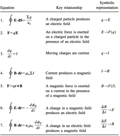
Figure 2.3.1: Key relationships of E&M (table taken from Bagno and Eylon, 1997) …….. 18
Figure 3.3.1: Average equation usages in all the E&M chapters ………. 48
Figure 3.3.2: Wordle of all the E&M equations ………... 49
Figure 3.3.3: Wordle of physics equations from non-E&M chapters ……….. 50
Figure 3.3.4: Wordle of all the math equations ……… 50
Figure 3.3.5: Average number of equations needed for a problem in each chapter ………. 51
Figure 3.3.6: Average number of local equations needed for a problem in each chapter … 52 Figure 3.3.7: Average number of E&M equations from other chapters needed in each chapter ………... 53
Figure 3.3.8: Average number of non E&M equations needed in each chapter …………... 53
Figure 3.3.9: Average number of math equations needed in each chapter ………... 54
Figure 3.3.10: Total out-of-chapter usage times of equations from each chapter ………… 55
Figure 3.3.11: Total usages of local equations in chapter 23 ……… 58
Figure 3.3.12: Total usages of local equations in chapter 24 ……… 68
Figure 3.3.13: Total usages of local equations in chapter 25 ……… 76
Figure 3.3.14: Total usages of top 10 local equations in chapter 26 ……… 81
Figure 3.3.16: Total usages of local equations in chapter 28 ……… 89
Figure 3.3.17: Total usages of local equations in chapter 29 ……… 94
Figure 3.3.18: Total usages of top 10 local equations in chapter 30 ……… 100
Figure 3.3.19: Total usages of local equations in chapter 31 ……… 103
Figure 3.3.20: Total usages of top 10 local equations in chapter 32 ……… 111
Figure 3.3.21: Total usages of top 10 local equations in chapter 33 ……… 117
Figure 3.3.22: Total usages of top 10 local equations in chapter 34 ……… 120
Figure 3.3.23: Percentage of each equation’s usage in all equations of chapter 27 ………. 131
Figure 3.3.24: The relations between chapters in edition 9 ……….. 135
Figure 3.4.1: Average equation usages in all the E&M chapters ……….. 138
Figure 3.4.2: Average number of equations needed for a problem in each chapter ………. 138
Figure 3.4.3: Average number of local equations needed for a problem in each chapter … 139 Figure 3.4.4: Average number of E&M equations from other chapters needed in each chapter ……….. 139
Figure 3.4.5: Average number of non E&M equations needed in each chapter …………... 140
Figure 3.4.6: Average number of math equations needed in each chapter ………... 140
Figure 3.4.7: Total out-of-chapter usages of equations from each chapter ……….. 141
Figure 3.4.8: Total usages of local equations in chapter 20 ……….. 143
Figure 3.4.9: Total usages of local equations in chapter 21 ……….. 145
Figure 3.4.10: Total usages of local equations in chapter 22 ……… 146
Figure 3.4.12: Total usages of top10 local equations in chapter 24 ………. 150
Figure 3.4.13: Total usages of top 10 local equations in chapter 25 ……… 151
Figure 3.4.14: Total usages of local equations in chapter 26 ……… 153
Figure 3.4.15: Total usages of local equations in chapter 27 ……… 154
Figure 3.4.16: Total usages of local equations in chapter 28 ……… 156
Figure 3.4.17: Total usages of local equations in chapter 29 ……… 158
Figure 3.4.18: Total usages of local equations in chapter 31 ……… 160
Figure 3.4.19: Total usages of local equations in chapter 35 ……… 161
Figure 3.4.20: The relations between chapters in edition 1 ……….. 165
Figure 3.5.1: Average equation usages of the two editions ……….. 167
Figure 3.5.2: Average usages of local chapter equations for all chapters in the two editions ………. 168
Figure 3.5.3: Average usages of out-of-chapter E&M equations for all chapters in the two editions ……… 169
Figure 3.5.4: Average usages of non E&M equations for all chapters in the two editions .. 170
Figure 3.5.5: Average usages of math equations for all chapters in the two editions …….. 171
Figure 4.2.1: Average number of sentences of problems in edition 9 ……….. 182
Figure 4.2.2: Average number of tasks of problems in edition 9 ………. 183
Figure 4.2.3: Percentages of numerical problems in the edition 9 ……… 184
CHAPTER 1 Introduction
The purpose of this dissertation is to investigate the End-Of-Chapter problems in a popular introductory physics textbook to give insight into the properties of EOC problems in general and whether those properties have changed in the past decades. In this chapter, I will introduce my motivation for this study and describe the change in the problems from the book authors’ point of view.
1.1 Motivation For The Research
Problem solving has been one of the major domains of physics education research for decades, and many problems were used in those studies (see for example, Hsu, et al. 2004, Maloney, 1994 & 2011). Among all the different kinds of physics problems, End-of-Chapter (EOC) textbook problems were studied most thoroughly since those were the problems that students have been using mostly. Early problem solving studies have described the properties of the typical EOC textbook problems thoroughly enough that later researchers could easily chose EOC problems under that description for their studies. However, how well this
common impression of EOC problem really fits all EOC problems and whether the textbooks have changed their way of selecting problems need to be investigated.
equations from different parts of the book. Thus, it seems interesting to investigate how many of those problems already exist in textbooks and how different are the concepts used in those problems.
I also generalized my curiosity to other properties of EOC problems, and wanted to see if these problems have changed after being criticized by physics education researchers for decades.
An easy investigation can be made by looking into the Prefaces of different editions of a physics textbook. Descriptions of the book’s problems from the Prefaces of the 9 editions of Physics for Scientists & Engineers by Serway et al. (1982, 1986, 1990, 1996, 2000, 2004, 2008, 2010 & 2014) are listed below:
Edition 1:
The Preface described the exercises as “straight forward in nature and are intended to test the student’s basic understanding of the material” and the problems as “generally more challenging and usually involve several concepts”.
Edition 2:
Edition 3:
Added “laboratory problems” which allowed students to write solutions based on real data and “Spreadsheet Problems” which included a spreadsheet on a separate disk that would help students work some of the difficult problems.
Edition 4:
No major change mentioned in the Preface. Edition 5:
Stated that a substantial revision was made. Many of the new problems required students to make order-of-magnitude calculations.
Edition 6:
Stated a substantial revision was made. Added “Review Problems” requiring the student to combine concepts covered in the chapter with those discussed in previous chapters and “Paired Problems” some end-of-chapter numerical problems were paired with the same problems in symbolic form.
Edition 7:
Added “Not-just-a-number problems”: problems that required students to think qualitatively in some parts and quantitatively in others.
“Jeopardy! Problems”: practice in changing between different representations by stating equations and asking for a description of a situation to which they apply as well as for a numerical answer.
“Calculus-based problems”: applying ideas and methods from differential calculus or using integral calculus.
Edition 8:
Added “Biomedical problems”: problems related to biomedical situations. Edition 9:
Added “Impossibility problems”: the problem is a description of a situation and no
question is asked other than “Why is the following situation impossible?” in the beginning of the problem. The student must determine what questions need to be asked and what calculations need to be performed. Based on the results of these calculations, the student must determine why the situation described is not possible. This determination may require information from personal experience, common sense, Internet or print research, measurement, mathematical skills, knowledge of human norms, or scientific thinking. As shown above, the authors of this textbook had made many changes and added many different types of problems to the textbook across the editions. Thus, it was very reasonable to believe that some changes could be observed in my research results.
1.2 Research Questions
1. What and how are equations being used to solve End of Chapter problems in the Electricity &Magnetism chapters in most commonly used introductory calculus-based
textbooks?
2. Were there any differences between the first edition and the last edition of the textbook in terms of equation usages? If yes, what were the differences?
CHAPTER 2 Background
In this chapter, I will provide background in three areas related to the textbook problems: 1. How physics education researchers define the EOC problem and describe its
properties;
2. Alternative problems that were created to overcome the disadvantages of the EOC problems;
3. How textbooks and the problems in them have changed.
2.1 Physics Education Research on Problem Solving
Before defining EOC problems, the first term to be defined is “problem”. Newell and Simon gave one of the most frequently cited definitions. In their book (Newell & Simon, 1972), they defined problem as:
“A person is confronted with a problem when he wants something and does not know immediately what series of actions he can perform to get it.”
They further explained that:
“The desired object may be very tangible (an apple to eat) or abstract (an elegant proof for a theorem). It may be specific (that particular apple over there) or quite general
As we can see from the explanation, this definition of problem is quite generic. They further developed their problem solving theory basing on detailed discussion of three types of problems: Cryptarithmetic problem, Logic problem and Chess problem.
Another widely cited definition was given by John R. Hayes (Hayes, 1981). In his book discussing problem-solving skills, Hayes defined problem as
“Whenever there is a gap between where you are now and where you want to be, and you don’t know how to find a way to cross the gap, you have a problem.”
Along with the definition, he also provided a few short examples:
“If you are on one side of a river and you want to get to the other side but you don’t know how, you have a problem. If you are assembling a mail-order purchase, and the instructions leave you completely baffled about how to ‘put tab A in slot B,’ you have a problem. If you are writing a letter and you just can’t find the polite way to say, ‘No, we don’t want you to come and stay for a month,’ you have a problem.”
Clearly, the problems discussed in Hayes book covered a wide range of problems in general, including a few physics problems, for example:
“Who’s Got the Enthalpy? Liquid water at 212 °F and 1 atm has an internal energy (on an arbitrary basis) of 180.02 Btu/lbm. The specific volume of liquid water at these conditions
is 0.01672 ft3/lbm. What is its enthalpy?”
depends on the problem solver’s ability to solve the problem, some situations might qualify as a problem to some people but not qualify as a problem for others.
In studies of problem solving, physics problems were used from time to time. For example, Bhaskar and Simon (1977) used six chemical engineering thermodynamics problems in their study of problem solving behavior. They provided an example for the problems used in the study:
“Nitrogen flows along a constant area duct. It enters at 40 °F and 200 psi. It leaves at atmospheric pressure and at a temperature of -210 °F. Assuming that the flow rate is 100 lb/min, determine how much heat will be transferred to the surroundings.”
A larger sample of physics problems was used in Michelene T. H. Chi’s landmark paper (Chi, Feltovich and Glaser, 1981) on knowledge organization. This paper included four studies, the first study used 24 problems selected from Halliday and Resnick’s (1974) Fundamentals of Physics, another 20 problems were constructed for study 2 and 4. Most of those problems included a diagram, and they were all typical textbook problems.
David P. Maloney (Maloney, 1994) circularly defined this type of physics problem as: “The kind of task that is usually found at the ends of the chapters in introductory college physics books.”
He further described it as:
possible variables is to be determined. These tasks are very specific and well defined, since only relevant variables are included and the unknown is explicitly identified.”
According to this definition, End-Of-Chapter (EOC) problem was basically defined by its literal meaning. The description given by Maloney restricted the EOC problems into a very specific type, and the EOC problems used in the early studies all fit well into that type.
If we remove the restriction of typical textbook problems and look at all physics problems, the features of the problems could have larger diversity.
The textbook problems are well-defined problems, but problems in general could also be ill-defined. Simon (1973) discussed the definition of “ill-structured problems” and the boundary between well-structured and ill-structured problems. Since then, many physics problems that fall into the category of ill-defined problem have been introduced (Maloney and Coll, 1987; Voss, 1989, Heller and Hollabaugh, 1992; van Heuvelen and Maloney, 1999; Styer, 2011).
(2006) provided examples of types of chemistry textbook problems for each of the eight types. Apparently, chemistry textbook problems have larger diversity on this spectrum than physics textbook problems.
Maloney’s description also seemed to restrict the EOC problems to numerical problems, but physics problems could have more representations than numerical (Larkin, 1983; van Heuvelen, 1991). Representations can be categorized in many ways, Meltzer (2005) divided physics problems into four main categories: Verbal, Diagrammatic, Mathematical and Graphical. Kohl and Finkelstein (2005, 2006 & 2008) also used these categories but changed the name of a category from Diagrammatic to Pictorial.
Teodorescu and et al. (2013) classified physics problems by six levels of the student’s consciousness of processing using their Taxonomy of Introductory Physics Problems (TIPP). They identified that textbook problems all belonged to the lower four levels but they believed that the higher levels (Self-system and Metacognitive system) are also important for physics problem solving.
This study focuses on common EOC problems since they are the problems that students are using most. However, many studies showed that the typical textbook problems were not ideal.
still had some commonly seen difficulties in understanding basic concepts of mechanics even after solving an average of 1500 textbook problems. The study also showed that there was little correlation between conceptual understanding and the number of problems solved.
More importantly, solving problem is supposed to improve students’ problem solving abilities, but EOC problems didn’t seem to meet that expectation. The students, normally considered as novice problem solvers, used a “means-end” approach when solving the problem and turned the problem into a “plug-and-chug” game (Simon and Simon, 1978; Redish, Scherr and Tuminaro, 2006). Students used a heavy load of their cognitive resources on that approach and made their cognitive processing capacity consequently unavailable for other cognitive activities (Sweller, 1988). Garrett et al. (1990) argued that the EOC problems are exercises instead of problems (because the solution path is instantly known) and
suggested converting them into open-ended tasks.
2.2 PER-Based Problems Vs. Textbook Problems
Since the traditional EOC problems have limitations, researchers introduced alternative problem types to provide better learning outcomes.
Ranking Tasks
Ranking Task was to rank a series of eight situations of a moving car on the strength of the forces that will be needed to stop the car in the same distance.
Active Learning Problem Sheet (ALPS)
ALPS (van Heuvelen, 1991; van Heuvelen, 1996) was an approach that breaks problems into multiple manageable steps so that students can use it in the early stage of their learning process (for example, during a class). The problems intensively used multiple representations and included a variety of tasks.
Context-Rich Problem
Context-rich problems were designed to encourage students to practice an expert-like problem-solving strategy (Heller and Hollabaugh, 1992). This type of problem combined many aspects:
1. It was a real-world problem so that students would see it less as a mathematical manipulation of formulas.
3. The problem statement normally didn’t specify the unknown variable so the student needed to determine what the target variable was.
4. The problem was normally in one piece and didn’t have tasks in series. They argued that breaking problem into multiple steps would provide hints for students’ decision making in the solving process.
An example provided in the paper was the following problem: Traffic ticket: Introductory physics problem
While visiting a friend in San Francisco, you decide to drive around the city. You turn a corner and find yourself going up a steep hill. Suddenly a small boy runs out on the street chasing a ball. You slam on the brakes and skid to a stop, leaving a skid mark 50 ft long on the street. The boy calmly walks away, but a policeman watching from the sidewalk comes over and gives you a ticket for speeding. You are still shaking from the experience when he points out that the speed limit on this street is 25 mph.
Jeopardy! Problem
Jeopardy! Problem was a type of physics problem that was designed by reversing the solving process of a traditional physics problem (van Heuvelen and Maloney, 1999). The students were presented with a part of the solution (an equation, a diagram or graph) and were asked to create the problem using it. One example given in the paper was starting from an equation “12 V = I {[1/(5 Ω+ 6 Ω) + 1/(8 Ω)]-1 + 14 Ω]}, the task was to draw an electric circuit corresponding to that equation.
Problem Posing
Find-the-Flaw Problem
This type of problem (Styer, 2011; Grimvall, 2012) asked students to identify incorrect answers without actually solving the problem. It was open-ended because the solution involved not just pointing out which answers were wrong but explaining why they were incorrect. The solution of these problems could include dimensional analysis, approximation, numerical estimation and other skills.
Synthesis Problem
Ding and et al. (2011) argued that the EOC problems were “localized, addressing only material covered in a single chapter” which encouraged students to look locally for formulas instead of searching for underlying concepts. They introduced Synthesis Problems to address this issue. These problems were designed to contain multiple concepts from broadly
Figure 2.2.2: An example of synthesis problem (from Ding, et al., 2011)
2.3 Research on Introductory Textbooks
The first aspect about textbooks that relates to my study would be the contents delivered in the book, especially the E&M part.
However, teaching outcomes of the traditional introductory level classes were not very good, as students’ conceptual understanding was typically quite poor (Maloney, 2001). Thus, some studies suggested different teaching approaches.
Galili and Kaplan (1997) suggested a new approach emphasizing the complementarity of electric and magnetic fields. The approach treats these fields in a similar manner that is consistent with mechanics in an effort to improve the integrity and self-consistency of the course.
Chabay and Sherwood (2006) suggested a new way of arranging topics in order to emphasize fundamental principles. By connecting field concepts to concrete microscopic models of matter, this sequence can increase the effectiveness of teaching basic concepts and also avoid early introduction of Gauss’s law and Faraday’s law.
PER studies have made many suggestions to book authors, but it is not known whether the EOC problems of textbooks have changed. This is because a quantitative study that shows the change of EOC problems of a textbook is missing.
physics textbooks, but he compared the conceptual content of the texts as well as the distribution of conceptual problems in those textbooks (close, but still not the EOC problems).
CHAPTER 3 Part 1: The Study of Equations 3.1 Research Method
3.1.1 Selecting the EOC Problems
The objects of study in this research project are the End-Of-Chapter Problems of a popular introductory-level physics textbook. The first task of the study was to choose appropriate problems.
I used Physics for Scientists and Engineers with Modern Physics by Serway and Jewett (Editions 1 to 9) for this study. I chose a calculus-based textbook instead of algebra-based because books with this level of mathematical sophistication are normally written for Science and Engineering students and so might have more complex EOC problems. Secondly, this textbook has been very widely used in the past decades. In a study in 1996 (Amato, 1996), this book had been listed as one of the most popular texts. Even though publishers don’t normally reveal their marketing information, the fifth edition of this textbook was said to be the top-seller of all physics textbooks in 2000 (Beichner, 2005). Thirdly, the nine editions of this textbook were released from 1980 to 2015, which matches a period of rapid expansion of physics education research (PER) and its implications for instruction. Most relevant here, many important studies on problem solving (see, Maloney, 2011) were published during this time.
chapters into six parts: Mechanics, Oscillations and Mechanical Waves, Thermodynamics, Electricity and Magnetism, Light and Optics, Modern Physics. Among those six parts, only the 12 chapters in Electricity and Magnetism are analyzed in this study.
Table 3.1.1: E&M chapters in all the editions
Editions 1st 2nd 3rd 4th 5th 6th 7th 8th 9th
Electricity and Magnetism
Electric Fields è è è è è è è è
Gauss's Law è è è è è è è è
Electric
Potential è è è è è è è è
Capacitance
and Dielectrics è è è è è è è è
Current and
Resistance è è è è è è è è
Direct-Current
Circuits è è è è è è è è
Magnetic Fields è è è è è è è è
Sources of the
Magnetic Field è è è è è è è è
Faraday's Law è è è è è è è è
Inductance è è è è è è è è
Magnetism in
Matter
Alternating-Current Circuits è è è è è è è è
Electromagnetic
Waves è è è è è è è è
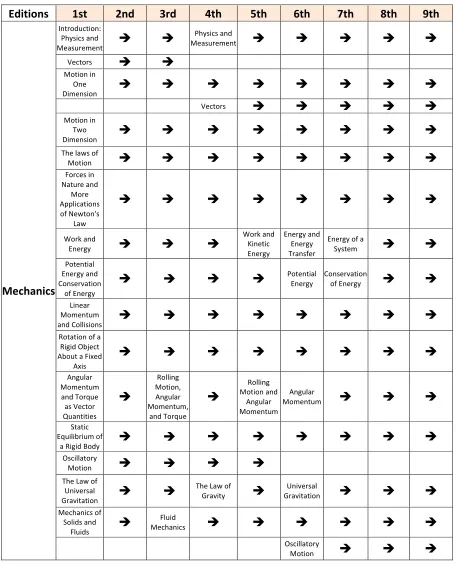
used in all of those 12 chapters were mostly stable across the editions. In contrast to the E&M part, all the other five parts have been changed more than this part. Consider the Mechanics chapters for example, as shown in Table 3.2. It is clear that there were many changes in both the names of the chapters and their ordering. The change of chapter name might indicate change of its content and changing the order would impact the usage of its content in the later chapters. Basically, what this all come down to is this: the main reason for using only the E&M chapters in this study is because of their stability across different
editions.
Table 3.1.2: Mechanics chapters in all the editions
Editions 1st 2nd 3rd 4th 5th 6th 7th 8th 9th
Mechanics
Introduction: Physics and
Measurement è è
Physics and
Measurement è è è è è
Vectors è è
Motion in One
Dimension è è è è è è è è
Vectors è è è è è
Motion in Two
Dimension è è è è è è è è
The laws of
Motion è è è è è è è è
Forces in Nature and More Applications of Newton's Law è è è è è è è è Work and
Energy è è è
Work and Kinetic Energy Energy and Energy Transfer
Energy of a
System è è
Potential Energy and Conservation
of Energy
è è è è Potential Energy Conservation of Energy è è
Linear Momentum
and Collisions è è è è è è è è
Rotation of a Rigid Object About a Fixed
Axis è è è è è è è è Angular Momentum and Torque as Vector Quantities è Rolling Motion, Angular Momentum, and Torque è Rolling Motion and Angular Momentum Angular
Momentum è è è
Static Equilibrium of
a Rigid Body è è è è è è è è
Oscillatory
Motion è è è è
The Law of Universal
Gravitation è è
The Law of
Gravity è Gravitation Universal è è è Mechanics of
Solids and Fluids è
Fluid
Mechanics è è è è è è
25
An added benefit of focusing on the E&M chapters is that they normally serve as the main content for the second semester in introductory physics courses and the problems found in the E&M chapters sometimes use equations from previous mechanic chapters. This allows me to gather important information about far transfer of physics knowledge.
After choosing the chapters, it is also important to choose the end-of-chapter problems in the chapters. Normally, the end-of-chapter problems of this textbook are divided into two types by the authors, the conceptual (generally qualitative) questions and the more
quantitative problems. The first edition didn’t have conceptual questions. Starting from the second edition, those two types of problems were included and named as Questions and Problems respectively. Starting from the 8th edition, conceptual questions have been further divided into two categories: Objective Questions and Conceptual Questions. Despite the change in the names, what didn’t change is that all the Problems normally need at least one equation to solve while all the conceptual questions don’t normally need any equation to answer. In this examination of equations, I naturally choose only the Problems at the end of the E&M chapters in all the editions of Serway’s textbook as my objects of study. The name “EOC problems” will be referring to only those problems in this study.
It is important to point out some limitations about this problem bank. First of all,
first assumption is that the textbook is a good sample of typical EOC problems. I assume that EOC problem choices represent the authors’ best attempt to keep the percentages of all the different problems suitable to their requirements. Secondly, I need to also point out that the problem set I used here might not be the actual problem set assigned to the students as their homework. It is very common that instructors would only select a subset of problems from the textbook as homework assignments. So the problem set in this study is the set that
students have access to, but almost certainly not the set they get to work on. Thus, my second assumption is that the complete problems set in the textbook is a good sample of the problem set that the student’s actually get to work on. I assume it is the authors’ and the instructors’ mutual intention to keep the percentages of different problems appropriate for both students’ textbook and their homework. Basing on those two assumptions, I assume the problem bank I choose in my study is a good representation of EOC problems in general.
3.1.2 The Solutions of the Problems
To code the equations that need to be used in solving all the problems, I first wrote down the solution(s) for each problem. (It was sometimes possible to solve a problem by more than a single method.) I tested the reliability of the solutions by comparing my solutions to the solutions provided in the Worked Examples (the example problems and solutions within the body of each chapter provided by the authors) of the textbook (9th edition).
Worked Examples without seeing the authors’ solution. Then I compared my solutions to the solutions provided in the textbook.
There are a total of 90 Worked Examples in the E&M chapters of the 9th edition. Four of the Worked Examples (24.6, 28.8, 31.5 and 34.4) are conceptual problems and don’t need any equations in the solution, so I excluded them from the comparison. For the remaining 86 Worked Examples, my solutions agree with the solutions of the textbook in 74 Worked Examples. I will discuss the other 12 Worked Examples case by case in the following three categories:
1. I use equations that were introduced after the Worked Example in the chapter: 3 Problems (28.1, 30.6 and 32.1)
Worked Example 28.1
“A battery has an emf of 12.0V and an internal resistance of 0.0500 Ω. It’s terminals are connected to a load resistance of 3.00 Ω.
(A) Find the current in the circuit and the terminal voltage of the battery.
(B) Calculate the power delivered to the load resistor, the power delivered to the internal resistance of the battery, and the power delivered by the battery.”
Worked Example 30.6 was a problem that asks for calculating the magnetic field of a toroid. It was inserted before Equation 9.8.7 “B of Toroid” was introduced.
Worked Example 32.1 was a problem that asks for calculating the inductance of a solenoid while I used Equation 9.10.3 “L of Solenoid” in my solution, which was included later in the Summary of the chapter.
In all of the above problems, I used an equation from the Summary part of the chapter. However, because the Worked Example was in earlier section of the context, it couldn’t use the later equation. It was clear that if the Worked Examples were given to anyone with access to all the available equations of the chapter, they would agree with my solution. So this issue wouldn’t be a problem for my study of the EOC problems as all equations of the chapter were introduced before them.
2. Solutions had differences in the number of times of equation usage: 2 problems (26.4 and 26.7)
Both problems involved two capacitors and the situations for the two capacitors were identical in the problems.
In Worked Example 26.4 where the problem needed the total charge of two capacitors, one solution was to use Equation 9.4.1 “C=Q/V” twice to calculate the charge on each
same result on the other capacitor since they were identical. In both cases, the types of equations were same for both methods. The only difference was the number of times where one equation got to be used. In Section 3.2, I will describe a pilot study I conducted to show why I didn’t track the number of multiple usages of the same equation in one problem. Thus this issue wouldn’t make a difference in my data.
3. The problem could be solved by more than one method: 7 problems (25.4, 28.4, 28.7, 29.3, 30.4, 31.6 and 33.1)
This was a more common type of issue about the reliability of my solution. I will discuss it in the following three situations:
(1) One of the two methods was more related to the current chapter than the other: 2 problems (25.4 and 29.3)
Worked Example 25.4—“The Electric Potential Due to a Dipole”:
The part (B) of this problem required calculation of the V and Ex at a point on the axis of
a dipole. The textbook’s solution used Equation 9.3.5 “E=-dV/dx” to get Ex from V. I agreed
with the solution, but I also identified another method of using Equation 9.1.4 “E of Multiple Charges” from chapter 23. However, I would argue that the additional method that I
Worked Example 29.3:
“In an experiment designed to measure the magnitude of a uniform magnetic field, electrons are accelerated from rest through a potential difference of 350V and then enter a uniform magnetic field that is perpendicular to the velocity vector of the electrons. The electrons travel along a curved path because of the magnetic force exerted on them and the radius of the path is measured to be 7.5 cm.
(A) What is the magnitude of the magnetic field? (B) What is the angular speed of the electrons?”
Part B of the problem asked for the angular speed of the electrons. So I naturally used Equation 9.7.5 “ω=qB/m” which was included in the Summary and should be used in particular for problems like this one. However, the textbook’s solution used Equation 9.0.38 “v=rω” which was an equation from chapter 10 which had not actually been covered yet. I would argue that my solution was more appropriate for the problem here in chapter 9.
In general, for the situation (1) where one method was more related to the current chapter, I would only code the method that uses equations from the current chapter because I consider it as closer to the purpose of have the problem in the chapter.
(2) The two methods ended up using the same set of equation codes. 3 problems (28.4, 28.7 and 30.4)
Equation 9.5.8 “R=V/I” to calculate the potential difference. However, the two methods had no differences in the equation codes.
Worked Example 28.7 was called “ A Multiloop Circuit” where it had a circuit of multi-loops, and required applying Equation 9.6.4 “Kirchhoff’s Loop Rule” along with some other equations. The two methods here differed on how to choose the loops, as there was more than one way to write down the Loop Rule. However, the two methods had no differences in the equation codes since they both need the same set of equations.
Worked Example 30.4 was called “Suspending a Wire” and it had two long wires carrying currents and applying a net force on a third wire. When calculating the net force on the third wire, there were two methods where one can either calculate the net B field first and then use Equation 9.7.6 “F=ILB” or use the Equation 9.7.6 first to calculate two forces and then combine them to get the net force. Either way, the equations codes of those two methods were both including Equation 9.7.6 and Equation 9.0.5 “Vector Calculation”.
(3) The two methods end up using different equations. 2 problems (31.6 and 33.1) Worked Example 31.6 was called “A Loop Moving Through a Magnetic Field” where a rectangular metallic loop moved into a uniform magnetic field with a constant speed, and the problem asked for the induced motional emf in the loop as a function of its position.
one side was cutting the field lines, one can use the Equation 9.9.3 “ε=-Blv” to calculate the induced emf by that side of the loop. Those two methods used different equations and both equations were introduced in the same chapter.
Worked Example 33.1:
“The voltage output of an AC source is given by the expression Δv = 200 sin ωt, where Δv is in volts. Find the rms current in the circuit when this source is connected to a 100 Ω resistor.”
This problem could be solved by first identifying the ΔVmax, then using Equation 9.11.5 “AC Ohm’s Law” to get I from ΔV. The issue arose when calculating the rms value from the maximum value. One method was to go from ΔVmax to ΔVrms and then use Ohm’s Law to get Irms. The other method was to get Imax first with Ohm’s Law and then go from Imax to Irms, so the codes would be a little different.
started with the EOC problems. Thus, I believe I can most likely write down all the alternative methods if there were any.
After that, I would code both of them with the related equation codes. Then I count each of the equation codes as used 0.5 times in the problem and add the codes together to be the final codes of the problem. In this way, for situation (2) I would have the same final code counts for either of the methods since they both use the same equations. For situation (3), my final code counts would be able to best represent both methods while not making the total number of equation codes larger than what it was actually used in either of the methods.
outside the chapter. In the end, I would expect my solutions for the EOC problems to be reliable.
It is important to point out here that the solutions that I will be using in this study don’t necessarily represent the solutions that an introductory level physics student might give, because students have a much higher chance of creating incorrect solutions for the problems than me. Even in their correct solutions, some unnecessary equations might be added. So future studies should be conducted to look into what equations students actually use to solve all the EOC problems in this textbook, but that is not the purpose of this research.
3.1.3 The Equation Codes
1. How were the equation codes generated?
In short, I didn’t generate the equations, I only named them. In Appendix A, I listed all the equation codes. The Code Names were assigned in order to give anyone with solid
physics knowledge an impression of which equation this code refers to. Meanwhile, the Code Names were also kept short and in one line for using in figures and tables. In order to keep them simple, some of the equations were named directly by the equation (for example, Equation 9.5.5 “J=I/A”), but some more complicated ones were named by its function (for example, Equation 9.1.3 “E of Point Charge”).
problem, I made sure all the equations being used to get it were included in my codes. In this way, I ensured that the set of equation codes I ended up with was complete enough for the purpose of solving the EOC problems on this textbook.
I started by including all the equations listed in the Summary part of each chapter. Those equations were listed as important by the textbook authors, and they were indeed all being used in the EOC problems.
Next, I identified equations that were introduced before the Summaries and were crucial for solving the EOC problems even though they were not listed in the Summary. All those equations were listed in Appendix A with a “*” to distinguish them. As an example, Equation 9.1.12 “Field Line Equation” was not included in the Summary of chapter 23, but the field line problems would be unsolvable without using this equation. Another example was Equation 9.1.10 “E of Ring” which the textbook authors derived with detailed steps of integration in the textbook. In an EOC problem that involves a uniformly charged rod, although it is still doable to start from the beginning and derive this result again, using the result of Equation 9.1.10 was clearly the purpose of the problem.
In addition to E&M equations, I also identified some equations that were not introduced in those chapters. I divided these into non-E&M physics equations and math equations, as shown in Appendix A.
A few non-E&M physics equations that are worth mentioning are listed below. (1). Equation 9.0.52 “Dimensional Analysis”:
Problem 25.45:
A rod of length L (Fig. P25.45) (Original figure not included here) lies along the x axis with its left end at the origin. It has a nonumiform charge density λ = αx, where α is a positive constant. (a) What are the units of α? (b) Calculate the electric potential at A.
As shown in the example above, this equation was actually on the units of another equation. In this case, “ C/m = [units of α] m”.
(2). Equation 9.0.53 “Cost =Price*Units”:
This equation was used when a total cost needed to be calculated. In the case of E&M problems, normally it involves the bill from the electric utility company.
Although this equation didn’t look like an equation in physics, it does involve physics quantities (electric energy) in it. Also, because the price was normally given as “$0.110 per kWH” and the equation was not given in the textbook, it required some “Dimensional Analysis” skills in order to figure out what equation should be used to calculate the cost.
(3). Equation 9.0.54 “Ignorable Ratio”
Problem 23.83:
A 1.00-g cork ball with charge 2.00 µC is suspended vertically on a 0.500-m-long light string in the presence of a uniform, downward-directed electric field of magnitude E = 1.00 × 10⁵ N/C. If the ball is displaced slightly from the vertical, it oscillates like a simple pendulum. (a) Determine the period of this oscillation. (b) Should the effect of gravitation be included in the calculation for part (a)? Explain.
In this example, to decide whether gravitation was ignorable, an equation showing the ratio of the two forces to be smaller than a certain value was needed. That equation should be coded with this equation code.
Although having this code was necessary, it’s not very clear where this equation came from in the textbook. In the chapter 1, when talking about Significant Figures, the textbook claims that it requires three significant figures for any answer. That might be an indication that the ignorable ratio is 1/1000. But I would rather attribute this equation code to page 465, where the textbook, for the first time, did an approximation on the accuracy of less than 1.0%. That example made the ignorable ratio to be 1/100 for this book.
(4) Equation 9.0.55 “Given Physics Equation” and Equation 9.M.28 “Given Math Equation”:
Problem 25.66:
A uniformly charged filament lies along the x axis between x = a = 1.00 m and x = a + l.00 m and x = a + l = 3.00 m as shown in Figure P25.66 (Original figure not included here). The total charge on the filament is 1.60 nC. Calculate successive approximations for the electric potential at the origin by modeling the filament as (a) a single charged particle at x = 2.00 m, (b) two 0.800-nC charged particles at x = 1.5 m and x = 2.5 m, and (c) four 0.4.00-nC charged particles at x = 1.25 m, x = 1.75 m, x = 2.25 m, and x = 2.75 m. (d) Explain how the results compare with the potential given by the exact expression
V = keQ
l ln l+a
a ⎛ ⎝⎜ ⎞⎠⎟
This example showed a problem with an additional equation in it. The equation was actually used in the solution because in order to explain part (b), the problem solver needed to calculate a potential using that equation. So it did qualify for an equation code.
Problem 23.59:
Consider an infinite number of identical particles, each with charge q, placed along the x axis at distances a, 2a, 3a, 4a, … from the origin. What is the electric field at the
origin due to this distribution? Suggestion: Use 1+ 1 22 +
1 32 +
1
42 +!=
π2
6
As shown in the above example, a math equation was given in the problem and it was used for the solution. So it’s coded as Equation 9.M.28 “Given Math Equation”.
Other than those, some EOC problems in the textbook also have equations in the problem statement that shouldn’t be coded. For example:
Problem 24.69:
A slab of insulating material (infinite in the y and z directions) has a thickness d and a uniform positive charge density ρ. An edge view of the slab is shown in Figure P24.61 (Original figure not included here). (a) Show that the magnitude of the electric field a distance x from its center and inside the slab is E=ρx/ε0. (b) What If? Suppose an electron of charge –e and mass me can move freely within the slab. It is released from rest at a distance x from the center. Show that the electron exhibits simple harmonic motion with a frequency
f = 1
2π ρ
In this example, two equations were given. However, the problem solver would be able to get the results without them. The solution of the problem would be the same if we changed its questions to “What is the magnitude of the E field” and “What is the frequency”. Thus, this situation needs to be excluded from this equation code.
Details about some other equation codes will be discussed in section 3.3.2.
2. Is it reliable when using those codes?
Basically, once a solution is created, it is straightforward to code the equations. There are no subjective judgments to be made. The equations are mutually exclusive, although this might not be immediately obvious. For example, Equation 9.2.1 “E Flux” seems to be mixed up with Equation 9.2.2 “E Flux Integral Form”, but it was actually very clear that Equation 9.2.1 should be used for situation when the E-field was uniform everywhere on the area. Equation 9.2.2 should only be used for situations where Equation 9.2.1 doesn’t work. In fact, most of the E&M equations arguably originated from the Maxwell’s Equations, but we problem solvers still know the appropriate equations to use and almost never start from the more fundamental Maxwell’s Equations.
Again, if there were situations where alternative equations can be used. I would have indicated that there was more than one solution as discussed in section 3.1.1.
In short, this set of equation codes represent this textbook very well. It is not exactly the same as the set of equations as used in other textbooks, but there are many similarities so the results from this study would still be very insightful for introductory textbooks in general.
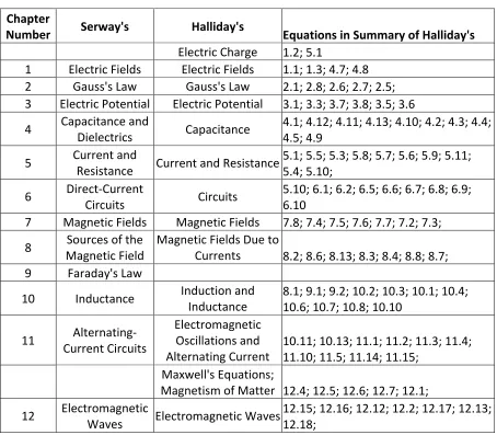
Perhaps the most obvious way various textbooks’ equations can vary is in the notations used for certain physical quantities. Take Fundamentals of Physics (7th edition) by Halliday, Resnick and Walker as an example. The “Coulomb’s Law” equation in that book is in scalar
formF= 1
4πε0
q1 q2
r2 while Equation 9.1.2 “Coulomb’s Law” here is in vector form, with different notations. But those differences don’t change the way the equations are used in solving problems, since the underlining physics is the same.
Secondly, the position of equations might be different in different textbooks. I will again use the Halliday, Resnick and Walker (HRW) book as an example. In that book, the
Table 3.1.3: Comparison of the Two Textbooks Chapter
Number Serway's Halliday's Equations in Summary of Halliday's Electric Charge 1.2; 5.1
1 Electric Fields Electric Fields 1.1; 1.3; 4.7; 4.8 2 Gauss's Law Gauss's Law 2.1; 2.8; 2.6; 2.7; 2.5; 3 Electric Potential Electric Potential 3.1; 3.3; 3.7; 3.8; 3.5; 3.6
4 Capacitance and Dielectrics Capacitance 4.1; 4.12; 4.11; 4.13; 4.10; 4.2; 4.3; 4.4; 4.5; 4.9
5 Current and Resistance Current and Resistance 5.1; 5.5; 5.3; 5.8; 5.7; 5.6; 5.9; 5.11; 5.4; 5.10;
6 Direct-Current Circuits Circuits 5.10; 6.1; 6.2; 6.5; 6.6; 6.7; 6.8; 6.9; 6.10 7 Magnetic Fields Magnetic Fields 7.8; 7.4; 7.5; 7.6; 7.7; 7.2; 7.3; 8 Magnetic Field Sources of the Magnetic Fields Due to Currents 8.2; 8.6; 8.13; 8.3; 8.4; 8.8; 8.7;
9 Faraday's Law
10 Inductance Induction and Inductance 8.1; 9.1; 9.2; 10.2; 10.3; 10.1; 10.4; 10.6; 10.7; 10.8; 10.10
11 Current Circuits Alternating- Electromagnetic Oscillations and
Alternating Current 10.11; 10.13; 11.1; 11.2; 11.3; 11.4; 11.10; 11.5; 11.14; 11.15; Magnetism of Matter 12.4; 12.5; 12.6; 12.7; 12.1; Maxwell's Equations;
12 Electromagnetic Waves Electromagnetic Waves 12.15; 12.16; 12.12; 12.2; 12.17; 12.13; 12.18;
Then, I used the equation codes of Serway’s book to code the equations in the Summary part of Halliday’s book and listed the code numbers Table 3.1.3 (for simplicity, code
numbers like 9.3.2 had been shorten to be 3.2). There were equations in HRW that didn’t have a corresponding code (for example, “Curie’s Law” equation), which could be considered as extra content found in only Halliday’s book. There were 60 E&M equation codes that didn’t show up in the Summaries of HRW, but those equations might be included in the book and not listed in its Summaries.
To see if the equation positions are mostly similar, I only looked at those equation codes that I identified. It is a subset of my equation codes, but it’s still a fairly large sample for my complete set of equation codes. Out of the 95 equation codes that I identified, 80 of them are still in their corresponding original chapters. This means about 84% of equations from Serway’s book are likely to be in the same corresponding chapter in Halliday’s book. In addition, if I don’t divide the equation codes in that table and make it one list, only 3 codes (5.1, 4.7 and 4.8) were in incorrect order. This means that about 97% of equations from Serway’s book might still be introduced in the same order in Halliday’s book.
To sum up, the equation codes used in this study are reliable and most of the results are expected to be generalizable to other introductory textbooks.
3.2 Pilot Study: Should We Count A Single Equation Multiple Times? 3.2.1 Pilot Study: Method
To get an idea of the outcomes I could expect if I counted multiple times when the same equation was reused in a problem, I conducted a pilot study on the first chapter of the first edition.
There were a total of 48 EOC problems in the chapter. The equations codes were the same as shown in Appendix A, except Equation 9.1.3 and Equation 9.1.4.
The Equation 9.1.3 was “E of Point Charge” and Equation 9.1.4 was “E of Multiple Charges”. This pilot study needed to count the number of usage for equations, but Equation 9.1.4 might be considered as multiple usages of Equation 9.1.3. To avoid this ambiguity, those two codes were combined to be the equation code “E of Particle Charge”.
3.2.2 Pilot Study: Results
Table 3.3 below shows the number of total usages of each equation code and how many problems they were used in. Equations’ average usage times in a problem were also
calculated.
Table 3.2.1: Equation Usage in Chapter 20 Edition 1
Equation
Codes E-Field to Force Coulomb's Law E of Particle Charge E of Continuum Charge Surface Charge Density Linear Charge Density Field Line Equation Problems used the
code 12 7 15 4 1 5 2
Total Usage 14 13 40 5 1 5 2
Average
Times 1.17 1.86 2.67 1.25 1.00 1.00 1.00
Equation
Codes E of Rod E of Disk E of Ring a=qE/m Total
Other Physics Equations Math Equations Problems used the
code 3 3 2 6 60 35 19
Total Usage 4 6 5 6 101 38 19
Average
Times 1.33 2.00 2.50 1.00 1.68 1.09 1.00
From the table 3.2.1 we can see that there were a few equations that stand out more likely to be used multiple times.
problem that was using it. “E of Ring” also got average usage times of 2.5. On the other hand, the important “E-Field to Force” Equation only had average usage times of 1.17. Equations like “Linear Charge Density” and “Field Line Equation” were only used once in each problem that needed them.
There were mainly two situations where equations would be used multiple times. The first was when there are many similar objects in the problem. In this chapter, problems that had multiple point charges would increase the usage times. For example, Exercise 15 of the chapter included three point charges and used Equation “E of Particle Charge” twice on each of the particles. The second situation was when problems had multiple questions and the questions were asking for repeating calculations. For example, Exercise 20 asked to calculate the E-field on the axis of a ring for four different distances. That problem alone contributed to the large number of average usage times of the equation “E of Ring”.
3.2.3 Pilot Study: Conclusion
By comparing the results between counting multiple usages and not counting multiple usages of equations, we can see that it makes a large difference. If counting the equations by multiple usages, then some equations might be over-represented in the final result. Also, counting multiple usages will dilute the usage of equations from outside the chapter.
If we consider the problem solving process, coding whether or not an equation is used is coding the problem solver’s decision making of choosing correct equations for the problem. On the other hand, coding the number of times that an equation is used is more likely to be coding the number of practices on the calculation of the equation.
As a result, for the purpose of my research, I had decided not to count multiple usages of the same equation in a problem.
3.3 The Latest Edition
3.3.1 Overall Equation Frequency
The 9th edition of the textbook has a total of 965 EOC problems in all the 12 E&M chapters. There were a total of 155 equation codes identified from the E&M chapters and 54 additional equation codes identified from non-E&M chapters.
E&M chapters and 0.55 ± 0.05 math equations. Figure 3.3.1 shows the average equations needed for solving the EOC problems in all the E&M chapters.
Figure 3.3.1: Average equation usages in all the E&M chapters
What were the most useful equations?
Notice that the first two categories were both E&M equations, so the average number of E&M equations for each problem was 2.15. Based on the total usages of each E&M
equations, I created a Wordle picture (Feinberg, 2010) shown in Figure 3.3.2, where the area taken by each equation was proportional to its total usage. For easy reorganization, equations showed in the Wordle were in their original forms in the textbook, not the equation codes (original equations for each code can be found in Appendix A).
Equabons From Local Chapter
Equabons From Other E&M Chapters
Equabons From Non-E&M Chapters
Figure 3.3.2: Wordle of all the E&M equations
Obviously, some equations were used more frequently than others. Equation 9.5.8 “R=V/I” was used most among all the equations. Details on why those equations got to be used so many times will be discussed in sections 3.3.2 and 3.3.3.
Figure 3.3.3: Wordle of physics equations from non-E&M chapters
In addition, there was also 0.55 math equations used in the EOC problems. Figure 3.3.4 shows a Wordle picture of those equations and their popularity is indicated by their size (scales of different Wordle images in this section are all different, and are chosen to better fit the size of its own equations).
Details about why some of those equations were used many times in the E&M chapters will be discussed in later sections.
How many equations did each of the chapters use?
The average number of all equations needed for solving an EOC problem in each chapter ranged from 2.87 to 4.32.
Figure 3.3.5: Average number of equations needed for a problem in each chapter
As shown in Figure 3.3.5, it was kept very consistent that about 3 to 4 different equations on average were needed to solve a problem in all those chapters. In the results I am going to show later, the fluctuations for average numbers of different types of equations needed in each chapter were much larger than this. Thus, the stable value of total equations needed is actually reflecting the general level of complexity for EOC problems.
The usages of E&M equations from the local chapter ranged from 0.99 to 3.26.
Figure 3.3.6: Average number of local equations needed for a problem in each chapter
From Figure 3.3.6 we can see that the AC Circuits chapter used the most local equations while the Faraday’s Law chapter used the fewest local equations.
The usages of E&M equations from other chapters ranged from 0 to 1.72. 0.00
Figure 3.3.7: Average number of E&M equations from other chapters needed in each chapter
From Figure 3.3.7 we can see that the Faraday’s Law chapter used the most of E&M equations from outside of the chapter.
The usages of non E&M equations ranged from 0.08 to 1.47. 0.00
0.50 1.00 1.50 2.00 2.50
From Figure 3.3.8 we can see that the Electromagnetic Waves chapter used the most of non E&M equations while the DC Circuits chapter used the fewest non-E&M equations.
The usages of Math equations ranged from 0.16 to 1.01.
Figure 3.3.9: Average number of math equations needed in each chapter
From Figure 3.3.9 we can see that the Gauss’s Law chapter used the most math equations while the DC Circuits chapter used the fewest Math equations.
Details about why each of the chapters used those numbers of equations will be discussed in the next section.
How did each of the chapters’ equations contribute in later chapters? The usefulness of each chapter’s equations for later chapters varied largely.
Figure 3.3.10: Total out-of-chapter usage times of equations from each chapter From Figure 3.3.10 we can see that equations form the Current and Resistance chapter were used most in later chapters while equations from the last four chapters were almost only for the chapter themselves (partly because fewer chapters followed them, partly because the topics were isolated, will be discussed in section 3.4).
Details about this result will be discussed in section 3.3.3.
3.3.2 Equations Usage Within Chapters
In this section, I will discuss what equations had been used and how they were used in each of the chapters. In order to better show the usage of equations in the EOC problems, I used my coding results to identify some Typical Problems to show the use of equations. I call it the “Equation Code plus Typical Problem” method. Before I go into my results of the study, let me first explain how this method works.
88
12
42 46 189
42 43 85
This “Equation Coding plus Typical Problem” method actually turned out to be an effective research tool that can help us to better understand equations. The general approach for using this method includes five steps:
1. Code the equations of a certain problem bank;
2. From the codes, identify the most common usages of a certain equation and identify the equations used together with it;
3. Identify Typical Problems (will be shown in the section, a list of Typical Problem can be found in Appendix B) in those usages and try to explain how and why the equation was used in the problem;
4. Go back to the codes and identify other equations that can potentially take the same role;
5. Explore why this equation was used more frequently than the other alternative ones. This method reveals two kinds of information: one is how and why equations are
normally being used, the other is how equations are relating to each other. I need to point out that it is not the code pattern that defines the equation, but rather the physics nature of
In this study, I only need to know the second kind of information and use it to understand how concepts from different parts of the book are used together for solving the EOC
problems. So in the following part, I only choose more Typical Problems for chapter 23 and 24 to showcase the power of this method and explain what I had learned about how and why equations were used. In later chapters, I will only provide Typical Problems to show some of the important relations between certain equations.
Typical Problems used in this study had 4 categories: Type 1 Problem, to show the usage of equations from local chapter; Type 2 Problem, to show the usage of equations from other E&M chapters; Type 3 Problem, to show the usage of equations from other physics chapters; Type 4 Problems, to show the usage of math equations. A complete list of Typical Problems can be found in Appendix B, where the original problem numbers in the textbook are also provided.
Chapter 23 Electric Fields
On average, the 91 EOC problems in this chapter used 2.87 ± 0.30 equations, including 1.24 ± 0.11 equations from the local chapter, 0 equations from other E&M chapters