Image Smoothing Via L0 Gradient Minimization

Image Smoothing Via L

Gradient Minimization

Sonali Dayal

M.Tech Scholar, Department of Computer Science, NVPEMI, Kanpur, Uttar Pradesh, India

ABSTRACT

We present a new image editing method,particularly effective for sharpening major edges by increasing the steepness of transition while eliminating a manageable degree of low-amplitude structures. The seemingly contradictive effect is achieved in an optimization framework making use of L0 gradient minimization,which can globally control how many non-zero gradients are resulted in to approximate prominent structure in a sparsity-control manner. Unlike other edge-preserving smoothing approaches,our method does not depend on local features,but instead globally locates important edges. It,as a fundamental tool,finds many applications and is particularly beneficial to edge extraction,clipart JPEG artifact removal,and non-photorealistic effect generation.

Keywords: L0 Smoothing, Edge Enhancement, Extraction Image Abstraction, Layer-Based Contrast Manipulation Edge Adjustment, Detail Magnification, Tone Mapping

I.

Photos comprise rich and well-structured visual information. In human visual perception, edges are effective and expressive stimulation, vital for neural interpretation to make the best sense of the scene. In manipulating and understanding pictures, high-level inference with regard to salient structures was intensively attended to. Research following this line embodies generality and usefulness in a wide range of applications, including image recognition, segmentation, object classification, and many other photo editing and non-photorealistic rendering tasks.

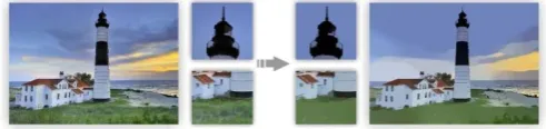
Figure 1. L0 smoothing accomplished by global

small-magnitude gradient removal. Our method suppresses low-amplitude details. Mean-while it globally retains and sharpens salient edges. Even the high-contrast

thin edges on the tower are preserved.

We in this thesis present a new editing tool, greatly helpful for characterizing and enhancing fundamental image constituents, i.e., salient edges, and in the meantime for diminishing insignificant details. Our method relates in spirit to edge-preserving smoothing [Tomasi and Manduchi 1998; Durand and Dorsey 2002; Paris and Durand 2006; Farbman et al. 2008; Subr et al. 2009; Kass and Solomon 2010] that aims to retain primary color change, and yet differs from them in essence in focus and in mechanism. Our objective is to globally maintain and possibly enhance the most prominent set of edges by increasing steepness of transition while not affecting the overall acutance. It enables faithful principal-structure representation.

(a) Abstraction (b) Pencil Sketch Rendering Figure 2. Our L0 smoothing results avail

Algorithmically, we propose a sparse gradient counting scheme in an optimization framework. The main contribution is a new strategy to confine the discrete number of intensity changes among neigh-boring pixels, which links mathematically to the L0

norm for information sparsity pursuit. This idea also leads to an unconventional global optimization procedure involving a discrete metric, whose solution enables diversified edge manipulation according to saliency. The qualitative effect of our method is to thin salient edges, which makes them easier to be detected and more visually distinct. Different from color quantization and segmentation, our enhanced edges are generally in line with the original ones. Even small-resolution objects and thin edges can be faithfully maintained if they are structurally conspicuous, as shown in Figure 1.

The framework is general and finds several applications. We apply it to compression-artifact degraded clipart recovery. High quality results can be obtained in our extensive experiments. Our method can also profit edge extraction, a fundamentally important operator, by effectively removing part of noise, unimportant details, and even of slight blurriness, making the results immediately usable in image abstraction and pencil sketch production, as shown in Figure 2.

(a) BLF [1998] (b) LCIS [1999] (c) WLS [2008]

(d) TV [1992] (e) Ours

Figure 2. Signal obtained from an image scanline, containing both details and sharp edges. (a) Result of

bilateral filtering. (b) Result of anisotropic diffusion used in the LCIS system. (c) Result of WLS optimization. (d) Result of TV smoothing. (e) Our L0

smoothing results.

In traditional layer decomposition, with an additional step to avoid structure over-enhancement, our method is applicable to detail enhancement based on separating layers, and possibly to HDR tone mapping after parameter tuning. We show several examples along with discussion of limitations that our method might cause over-sharpening for large illumination variation spanning dozens of pixels when strong smoothing is applied.

II.

Edge-preserving smoothing can be achieved by local filtering, including bilateral filtering [Tomasi and Manduchi 1998], its accelerated versions [Paris and Durand 2006; Weiss 2006;

Chen et al. 2007] and relatives [Choudhury and Tumblin 2003; Fattal 2009; Baek and Jacobs 2010; Kass and Solomon 2010]. Robust optimization-based approaches have also been advocated, represented by the weighted least square optimization [Farbman et al. 2008] and envelope extraction [Subr et al. 2009]. We discuss their properties using the 1D signal example (a scanline of a natural image) shown in Figure 2.

Farbman et al. [2008] proposed a robust method with the weighted least square (WLS) measure. The optimization framework with edge preserving regularization is more flexible compared with local filtering. Its result is shown in Figure 2(c). Another type of edge preserving regularization is total variation (TV) [Rudin et al. 1992], which is widely used to remove noise from images. It however also penalizes large gradient magnitudes, possibly influencing contrast during smoothing. One example is shown in Figure 2(d).

Subr et al. [2009] considered local signal extremes and used edge-aware interpolation [Levin et al. 2004; Lischinski et al. 2006] to compute envelopes. A smoothed mean layer is extracted by aver-aging the envelopes, originated from a 1D Hilbert-Huang transform (HHT). The method aims to remove small scale oscillations. Contrarily, our method targets globally preserving salient structures, even if they are small in resolution.

Kass and Soloman [2010] used smoothed histogram to accelerate local filtering and proposed the mode-based filters. Most recently,

Figure 3. Correspondence between k and 1/λ in Eqs. (2) and (3). The plot is obtained by trying different λ values in Eq. (3) and by finding the corresponding k

in the results after our optimization.

1D Smoothing

We enhance highest-contrast edges by confining the number of non-zero gradients, while smoothing is achieved in a global manner. To begin with, we denote the input discrete signal by g and its smoothed result by f . Our method counts amplitude changes discretely, written as

c(f) = #{p | | fp − fp+1| ≠ 0}, (1)

where p and p + 1 index neighboring samples (or pixels). | fp − fp+1| is a gradient w.r.t. p in the form of

forward difference. #{} is the counting operator, outputting the number of p that satisfies | fp − fp+1| ≠0,

that is, the L0 norm of gradient. c(f) does not count on

gradient magnitude, and thus would not be affected if an edge only alters its contrast. This discrete counting function is central to our method.

2D Formulation

In 2D image representation, we denote by I the input image and by S the computed result. The gradient ∇Sp

= (∂xSp, ∂ySp)T for each pixel p is calculated as color

difference between neighboring pixels along the x and y directions. Our gradient measure is expressed as

C (S) = # { p | |∂xSp| + |∂ySp| ≠0 } (4)

It counts p whose magnitude |∂xSp| + |∂ySp| is not zero.

With this definition, S is estimated by solving

In practice, for color images, the gradient magnitude |∂ Sp| is defined as the sum of gradient magnitudes in

rgb. The term ∑(S − I)2 _{constrains image structure}

similarity.

III.

Solver

Eq. (5) involves a discrete counting metric. It is difficult to solve because the two terms model respectively the pixel-wise difference and global discontinuity statistically. Traditional gradient decent or other discrete optimization methods are not usable.

problem. Our algorithm, due to the discrete nature, contains new subproblems. Both of them find their closed-form solutions. It is notable that the original L0-norm regularized optimization problem is known

as computationally intractable. Our solver is thus only an approximation, making the problem easier to tackle and upholding the property to maintain and enhance salient structures.

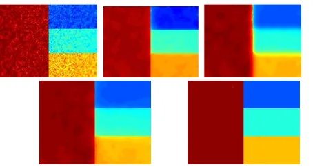
Figure 5. Noisy image created by Farbman et al. [2008]. (a) Color visualized noisy input. (b) Result of

Subr et al. [2009]. (c) Bi-lateral filtering (BLF) result (σs = 12, σr = 0.45) [Tomasi and Manduchi 1998]. (d)

Result of WLS optimization (α = 1.8, λ = 0.35) [Farbman et al. 2008]. (e) Our result.

We introduce auxiliary variables hp and vp,

corresponding to ∂xSp and ∂ySp respectively, and

rewrite the objective function as

(6)

where C(h, v) = # { p |hp| + |vp| ≠ 0 } and β is an

automatically adapting parameter to control the similarity between variables (h, v) and their corresponding gradients. Eq. (6) approaches (5) when β is large enough. Eq. (6) is solved through alternatively minimizing (h, v) and S. In each pass, one set of the variables are fixed with values obtained from the previous iteration.

Subproblems

Subproblem 1: computing S The S estimation subproblem corresponds to minimizing

∑ (

) (7)

by omitting the terms not involving S in Eq. (6). The function is quadratic and thus has a global minimum even by gradient decent. Alternatively, we diagonalize derivative operators after Fast Fourier Transform (FFT) for speedup. This yields solution

where F is the FFT operator and F()* _{denotes the}

complex conjugate. F(1) is the Fourier Transform of the delta function. The plus, multiplication, and division are all component-wise operators. Compared to minimizing Eq. (7) directly in the image space, which involves very-large-matrix inversion, computation in the Fourier domain is much faster due to the simple component-wise division.

Subproblem 2: computing (h, v) The objective function for (h, v)

where C(h, v) returns the number of non-zero elements in |h| + |v|. This apparently sophisticated subproblem can actually be solved quickly because the energy (9) can be spatially decomposed where each element hp and vp is estimated individually.

This is the main benefit of our splitting scheme, which makes the altered problem empirically solvable. Eq. (9) is accordingly decomposed to

Algorithm 1 L0 Gradient Minimization

Algorithm 1 L0 Gradient Minimization

Input: image I, smoothing weight λ , parameters β0,

βmax, and rate κ

Initialization: S ← I, β ← β0, i ← 0 repeat

With S(i)_{, solve for h(pi) and v(pi) in Eq. (12).}

With h(i) _{and v}(i)_{, solver for S}(i+1) _{with Eq. (8).}

Output: result image S

where H(|hp|+ |vp |) is a binary function returning 1 if

|hp|+ |vp| ≠ 0 and 0 otherwise. Each single term w.r.t.

pixel p in Eq. (10) is

Ep = (hp − ∂xSp)2 + (vp − ∂ySp)2 + λ/β H(|hp|+ |vp|) ,

(11)

which reaches its minimum Ep* under the condition

Proof.

1) When λ /β ≥ (∂xSp)2 + (∂ySp)2, non-

2) zero (hp, vp) yields

Ep((hp, vp) ≠ 0(, 0)) = (hp − ∂xSp)2 + (vp − ∂ySp)2 + λ /β ,

≥ λ /β ,

≥ (∂xSp)2 + (∂ySp)2.

(13)

Note that (hp, vp) = (0, 0) leads to

Ep((hp, vp) = (0, 0)) = (∂xSp)2 +

(∂ySp)2. (14)

Comparing Eqs. (13) and (14), the minimum energy

Ep* = (∂xSp)2 + (∂ySp)2 is produced

when (hp, vp) = (0, 0).

2) When (∂xSp)2 + (∂ySp)2 > λ /β and

(hp, vp) = (0, 0), Eq. (14)

Still holds. But Ep((hp, vp) ≠ 0(, 0))

has its minimum value

λ /β when (hp, vp) = (∂xSp, ∂ySp). Comparing these two

values, the minimum energy Ep*= λ /β is produced

when (hp, vp) =(∂xSp, ∂ySp).

With the above derivation, in this step, we compute for each pixel p the minimum energy Ep*. Summing

all of them, i.e., calculating ∑p Ep*, yields the global

optimum for Eq. (10).

Our alternating minimization algorithm is sketched in Alg. 1. Parameter β is automatically adapted in iterations starting from a small value β0, it is

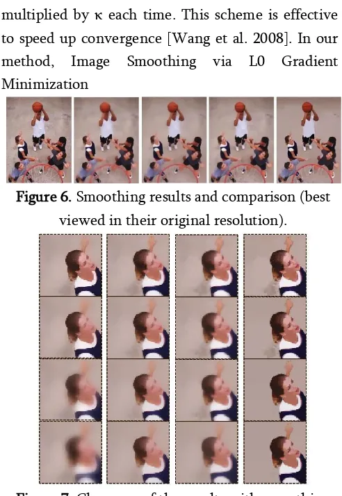
multiplied by κ each time. This scheme is effective to speed up convergence [Wang et al. 2008]. In our method, Image Smoothing via L0 Gradient Minimization

Figure 6. Smoothing results and comparison (best viewed in their original resolution).

Figure 7. Close-ups of the results with smoothing strength gradually increasing from top to bottom. (a)

Bilateral filtering (BLF) results. (b) Results of the WLS method. (c) Results of total variation smoothing.

(d) Our results.

β0 and βmax have fixed values 2λ and 1E5 respectively.

κ that is set to 2 is a good balance between efficiency and performance. We use this value to generate most of our results. Only in Figs. 6 and 11, we set it to 1.05 to allow more iteration in optimization, leading to higher-quality results. The critical parameter λ is allowed to be adjusted to effectively control the level of structure coarseness.

publicly available in the project website.

Comparison to quantization and segmentation To clarify the difference, we use the example shown in Figure 9, where the natural image contains a very small amount of noise, common in photos. Color quantization can neither suppress noise nor accurately remove details, yielding incorrect boundaries, as shown in Figure 9(b). Image segmentation seeks proper spatial partitioning. This set of methods are widely known as difficult to maintain fine edges, infective algorithm to achieve sub-problem global optimization are central to the high practicality.

Difference with total variation and other regularizers Continuous Lp norm with p = 1 was enforced in total

variation (TV) smoothing to suppress noise. In this framework, strong smoothing inevitably curtails originally salient edges to penalize their magnitudes. In our method, large gradient magnitudes are allowed by nature with our discrete counting measure.

Lp norm regularization with 0.5 ≤ p ≤ 1 was also

employed in [Levin et al. 2007] to model the sparsity of natural image gradients. The success of the WLS optimization attributes in part to the Lp norm in the

Iterative Reweighed Least Square (IRLS) framework.

Mathematically, Lp norm satisfies positive scalability

constraint , where a is a scalar.

It yields if |a| > 1, which implies that these norms still impose large penalties on salient gradients. On the contrary, the L0 norm in

Eq. (1) satisfies #{|x| > 0} = #{|ax| > 0} for any non-zero a, and thus does not comply with the positive scalability constraint. This major difference leads to new smoothing behavior.

Selectively penalizing image gradients is also related to the Weak Membrane model of Blake and

Zisserman [1987], which explicitly represents discontinuity and adjusts gradients only in continuous regions. Our method is dissimilar in formulation and in solver.

A natural image example is comparison with other state-of-the-art approaches. More are put in our project website, produced with different parameters. Close-ups are obtained by varying smoothing strength. Our results contain globally the most salient structures in different degrees.

Comparison to local histogram-mode filtering The method of Kass and Solomon [2010] is not based on smoothing neighboring pixels, and thus can sharpen edges while reducing details. We show in Figure 10 a close-up comparison. The edges in our result (b) are in line with the originally salient ones due to the global optimization.

IV.

Our method avails several applications due to its fundamentality and the special properties in processing natural images. We apply it to edge enhancement and extraction, non-photorealistic rendering, clipart restoration, and layer decomposition based manipulation. Following are some applications:

1. Edge Enhancement and Extraction 2. Image Abstraction and Pencil Sketching 3. Clip-Art Compression Artifact Removal 4. Layer-Based Contrast Manipulation 5. Edge Adjustment

6. Detail Magnification 7. Tone Mapping

V.

discretely counting spatial changes, which can remove low-amplitude structures and globally preserve and enhance salient edges, even if they are boundaries of very narrow objects.

As our system does not use spatial filtering or averaging, it can be regarded as complementary to previous local approaches. Interestingly, when combined with local filtering, our method can produce novel effects. Only bilaterally filtering the image contrarily blurs main boundaries under strong smoothing. We propose first applying bilateral filtering, which lowers the amplitudes of noise-like structures more than those of long coherent edges, followed by our method to globally sharpen prominent edges. Result in (d) only contains large-scale salient edges, profiting main structure extraction and understanding. To remove textures, our method may produce an over-sharpened result, as exemplified in (b). This result, however, can still be used in detail magnification. After edge adjustment as described in Sec. 4.4 and taking the result as the base layer, we magnify only details. The aforementioned parameter tuning for tone mapping is another limitation. Two-scale tone management for photographic look. ACM Trans. Graph. 25, 3, 637–645. [5]. BAEK, J., AND JACOBS, D. E. 2010.

Accelerating spatially varying gaussian filters. ACM Trans. Graph..

[6]. BLACK, M. J., SAPIRO, G., MARIMONT, D. H., AND HEEGER, D. 1998. Robust anisotropic diffusion. IEEE Transactions on Image Processing 7, 3, 421–432.

[7]. BLAKE, A., AND ZISSERMAN, A. 1987. Visual reconstruction. The MIT Press.

[8]. BOYKOV, Y., VEKSLER, O., AND ZABIH, R. 2001. Fast approximate energy minimization via graph cuts. IEEE Trans. Pattern Anal. Mach. Intell. 23, 11, 1222–1239.

[9]. CHEN, J., PARIS, S., AND DURAND, F. 2007. Real-time edge-aware image processing with the bilateral grid. ACM Trans. Graph. 26, 3, 103.

[10]. CHOUDHURY, P., AND TUMBLIN, J. 2003. The trilateral filter for high contrast images and meshes. In Rendering Techniques, 186–196. [11]. COMANICIU, D., AND MEER, P. 2002. Mean

shift: A robust approach toward feature space analysis. IEEE Trans. Pattern Anal. Mach. Intell. 24, 5, 603–619.

[12]. CRIMINISI, A., SHARP, T., ROTHER, C., AND PEREZ´, P. 2010. Geodesic image and video editing. ACM Trans. Graph. 29, 5, 134.

[13]. DABOV, K., FOI, A., KATKOVNIK, V., AND EGIAZARIAN, K. O. 2007. Image denoising by sparse 3d transform-domain collaborative filtering. IEEE Transactions on Image Processing 16, 8, 2080–2095.

[14]. DECARLO, D., AND SANTELLA, A. 2002. Stylization and abstraction of photographs. ACM Trans. Graph. 21, 3, 769–776.

[15]. DONOHO, D. 2006. Compressed sensing. IEEE Transactions on Information Theory 52, 4, 1289–1306.

[16]. DURAND, F., AND DORSEY, J. 2002. Fast bilateral filtering for the display of high-dynamic-range images. ACM Trans. Graph. 21, 3, 257–266.

decompositions for multi-scale tone and detail manipulation. ACM Trans. Graph. 27, 3.

[18]. FARBMAN, Z., FATTAL, R., AND LISCHINSKI, D. 2010. Diffusion maps for edgeaware image editing. ACM Trans. Graph.. [19]. FATTAL, R., AGRAWALA, M., AND

RUSINKIEWICZ, S. 2007. Multiscale shape and detail enhancement from multilight image collections. ACM Trans. Graph. 26, 3, 51. [20]. FATTAL, R. 2009. Edge-avoiding wavelets and

their applications. ACM Trans. Graph. 28, 3. [21]. KASS, M., AND SOLOMON, J. 2010. Smoothed

local histogram filters. ACM Trans. Graph. 29, 4.

[22]. LEVIN, A., LISCHINSKI, D., AND WEISS, Y. 2004. Colorization using optimization. ACM Trans. Graph. 23, 3, 689–694.

[23]. LEVIN, A., FERGUS, R., DURAND, F., AND FREEMAN, W. T. 2007. Image and depth from a conventional camera with a coded aperture. ACM Trans. Graph. 26, 3, 70.