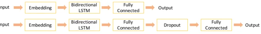
Figure 1: Architecture of modelm1(top) and modelm2(bottom)
Table 1: Statistics on the distance (in number of word tokens) betweenArg1andArg2in the ex-plicit relations in the training and test set of the PDTB Dataset (Prasad et al.,2008)
Distance Number of instances Percentage
0 3,554 22.29%
1 8,582 53.82%
2-10 1,743 10.93%
>10 2,066 12.96%
Total 15,945 100.00%
Table 2: Number of instances in the PDTB Dataset Dataset Explicit Non-Explicit Total Training 15,246 17,289 32,535
Testing 699 737 1,436
Total 15,945 18,026 33,971
the standard dataset in discourse parsing, thanks, in part, to the CoNLL shared tasks (Xue et al.,
2015, 2016). Using this corpus allowed us to compare our work with the state of the art sys-tems. The PDTB contains both explicit relations (marked with discourse connectives such as be-causeorbut) as well as non-explicit relations. Ta-ble2shows statistics of the dataset.
Since we focused on explicit relations only, the dataset was first cleaned by removing all non-explicit relations. As is standard in the field, we used sections 2-21 of the PDTB for training and section 22 was used for testing. Thus, about 15,246 instances such as example (1) in Section1
were used for the training process and 699 were used for testing.
4.2 Network Architecture
For our experiments, we used a neural network composed of Long Short-Term Memory (LSTM) cells (Hochreiter and Schmidhuber, 1997). An LSTM is a specialized form of a Recurrent Neu-ral Network (RNN) where a neuron is replaced with a memory cell. The memory cell is able to
learn and hold information to take into account long term dependencies, thus allowing to over-come the problem of vanishing and exploding gra-dients with RNNs (Hochreiter et al.,2001).
In order to learn the position ofArg1andArg2
and the length of these segments from the data only, we experimented with two main architec-tures. The first architecture shown in Figure 1
(top) is composed of an embedding layer that feeds directly into a Bidirectional LSTM layer. The Bidirectional LSTM layer is composed of 100 LSTM cells (for each direction) and the initial-ization is performed via the Glorot Uniform tech-nique (Glorot and Bengio, 2010). The Bidirec-tional LSTM outputs are then fed into a fully con-nected layer which outputs the probability of 4 possible labels: Arg1, Arg2, connective or
none for each input word. In the second archi-tecture, shown in Figure1 (bottom), we added a dropout layer as well as a fully connected layer at the end of the first model. This is shown in Fig-ure 1. We tested our architectures with different dimensions of word embeddings and decided to use a value of 300 as it resulted in a higher accu-racy with the training set (see Section4.3). Thus, this created the 2 models below:
1. m1: Bidirectional LSTM layer + vectors of 300 words
2. m2: Bidirectional LSTM layers + Dense + Dropout + Dense + vectors of 300 words
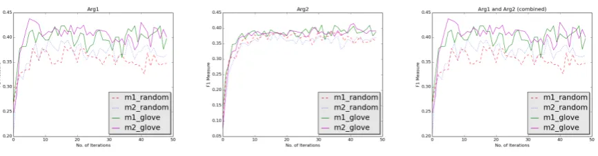
Figure 2: F1 score on the test set as a function of the number of iterations on the training set forArg1
(top),Arg2(middle) andArg1+Arg2(bottom)
We would have to waituntilwe have collected on those assets
[1, 2, 3, 4, 5, 6, 1, 7, 8, 9, 10, 11, 0, 0,..., 0]
Figure 3: Example with words in a training instance labelled with the corresponding numeric value
mean of the labels for an entire mini batch pro-vided in a single iteration.
4.3 Data Preparation
To provide as input to the neural networks, the training instances were converted into a numeric matrix structure. Since word embeddings are up-dated dynamically, we used pre-computedGloVe
embeddings (Global Vectors for Word Represen-tation) (Pennington et al.,2014) in one set of ex-periments and random values in another set. This was done by creating a dictionary of words and as-signing each word to a random numeric value. As shown in Figure3, a “zero word” was added to the vocabulary as a placeholder to pad sentences to an equal length. This length was set to 1,170 words, which is the size of the longest discourse segment containing bothArg1andArg2segments in the PDTB training dataset. Thus the input data was a 2 dimensional matrix of a fixed size of 300 by 1,170. The use of fixed size vectors was not a necessary requirement for the network, but it was mechanically easier to have consistency within the dataset. The label vectors were also correspond-ingly padded with the noneclass. This allowed the network to learn the end of theArg1+Arg2
sequence.
5 Results and Analysis
To evaluate our approach, we used the official CoNLL scoring module3 and modified it to
cal-culate the performance for explicit relations only. Specifically, the scoring module provides the scores for the exact match for Arg1only, Arg2
only andArg1+Arg2, for every instance in the test set.
For both models, the performance was evalu-ated at every epoch for a total of 50 evaluation points. Figure2shows the F1 scores of the models forArg1only,Arg2only andArg1+Arg2. As the graphs show, after about 10 epochs all models seem to stabilize and learn at a much slower rate hence reaching a saturation point.
Table 3 shows the performance of our ap-proaches compared to the state of the art sys-tems. As the table shows, hand-engineered ap-proaches still out perform our LSTM methods with F-measures between 55% to 46% for both
Arg1+Arg2. However, compared to (Wang et al., 2015), both m1 and m2 outperform their RNN approach which did incorporate some hand-engineered features. It is also worthwhile to note that pre-computed embeddings result in slightly higher F1 measures forArg1+Arg2than the ran-dom embeddings (25.75% versus 23.75% for m2
and 24.89% versus 22.75% form2) . This is most likely because of the sparsity of the words used
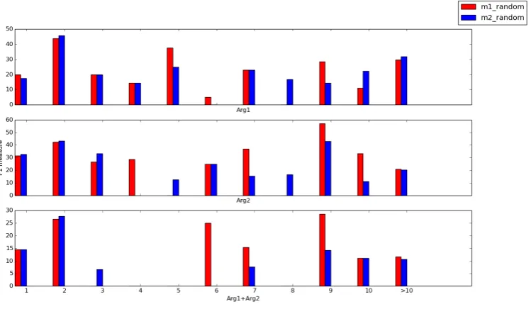
Figure 4: Plot of the distance-based F1 scores for Arg1 (top), Arg2 (middle) and Arg1+Arg2 (bottom)
in the dataset. Since not all words are equally weighted, the system is unable to learn the rela-tionship of those words in a given argument di-rectly from the dataset. Therefore, having pre-computed embeddings assist in optimizing the learning process for those words.
BecauseArg2is structurally bound to the con-nective, in the case of explicit relations, identify-ing the connective gives strong evidence to locate
Arg2. On the other hand, Arg1 is much harder to identify as it can be located in various posi-tions relative to Arg2. In the case of our LSTM based approach, it is interesting to note that while the F1 scores of Arg1 and Arg2 independently are quite lower than the state of the art, this dif-ference diminishes drastically for the combined
Arg1+Arg2F1 scores. This is because the neu-ral network optimizes over an entire instance and hence tries to maximize the score for both argu-ments combined as opposed to independently op-timizingArg1andArg2labeling.
To verify how our LSTM based approach han-dled long term dependencies, we separated the test dataset by distance and computed a distance-based F1 score. Recall from Section2that the distance is measured by the number of words between the closest words of Arg1 and Arg2 excluding the connective. Thus we count from the end ofArg1
to the start of Arg2or the connective whichever comes first whenArg1precedesArg2and from the end of Arg2 or the connective whichever
comes last to the start ofArg1 whenArg2 pre-cedes Arg1. Figure 4 shows the F1 scores for both the models learned with randomly initial-ized embeddings, calculated at their last epoch, as a function of the distance between Arg1 and
Arg2. It is interesting to note that while model
m1 randomseems to perform better on the longer distance based relations (greater than 9), model
m2 random still gets a better Arg1+Arg2 ac-curacy score. Moreover, both models do not show any correlation in their F1 measure as the distance increases. This indicates that both models are un-affected by long and short distances between the arguments of a discourse relation.
6 Conclusion and Future Work
ap-Jeffrey Pennington, Richard Socher, and Christopher D Manning. 2014. Glove: Global vectors for word
representation. InEMNLP. volume 14, pages 1532–
1543.
Rashmi Prasad, Nikhil Dinesh, Alan Lee, Eleni Milt-sakaki, Livio Robaldo, Aravind Joshi, and Bon-nie Webber. 2008. The Penn Discourse TreeBank
2.0. InProceedings of LREC-2008. Marrakech,
Mo-rocco.
Rashmi Prasad, Susan McRoy, Nadya Frid, Ar-avind Joshi, and Hong Yu. 2011. The
biomedi-cal discourse relation bank. BMC bioinformatics
12(1):188.
Rashmi Prasad, Eleni Miltsakaki, Nikhil Dinesh, Alan Lee, Aravind Joshi, Livio Robaldo,
and Bonnie L Webber. 2007. The Penn
Discourse Treebank 2.0 Annotation manual.
https://www.seas.upenn.edu/ pdtb/PDTBAPI/pdtb-annotation-manual.pdf.
Lianhui Qin, Zhisong Zhang, and Hai Zhao. 2016. Shallow discourse parsing using convolutional
neu-ral network. In (Xue et al.,2016), pages 70–77.
Niko Schenk, Christian Chiarcos, Kathrin Donandt, Samuel R¨onnqvist, Evgeny A Stepanov, and Giuseppe Riccardi. 2016. Do We Really Need All Those Rich Linguistic Features? A Neural
Network-Based Approach to Implicit Sense Labeling. In (Xue
et al.,2016), pages 41–49.
Nguyen Truong Son, Ho Bao Quoc, and Nguyen Le Minh. 2015. Jaist: A two-phase machine learn-ing approach for identifylearn-ing discourse relations in
newswire texts. In (Xue et al.,2015), pages 66–70.
Suzan Verberne, Lou Boves, Nelleke Oostdijk, and Peter-Arno Coppen. 2007. Evaluating discourse-based answer extraction for why-question
answer-ing. InProceedings of the ACM SIGIR. Amsterdam,
Netherlands, pages 735–736.
Jianxiang Wang and Man Lan. 2016. Two End-to-End Shallow Discourse Parsers for English and Chinese
in CoNLL-2016 Shared Task. In (Xue et al.,2016),
pages 33–40.
Longyue Wang, Chris Hokamp, Tsuyoshi Okita, Xiao-jun Zhang, and Qun Liu. 2015. The DCU discourse parser for connective, argument identification and
explicit sense classification. In (Xue et al.,2015),
pages 89–94.
Nianwen Xue, Hwee Tou Ng, Sameer Pradhan, Rashmi Prasad, Christopher Bryant, and Attapol Rutherford,
editors. 2015. The CoNLL-2015 shared task on
shal-low discourse parsing. Beijing, China.
Nianwen Xue, Hwee Tou Ng, Sameer Pradhan, At-tapol Rutherford, Bonnie Webber, Chuan Wang, and
Hongmin Wang, editors. 2016. The CoNLL-2016
Shared Task on Shallow Discourse Parsing. Berlin, Germany.
Yasuhisa Yoshida, Jun Suzuki, Tsutomu Hirao, and
Masaaki Nagata. 2014. Dependency-based
dis-course parser for single-document summarization. InEMNLP. Doha, Qatar, pages 1834–1839. Fang Kong Sheng Li Guodong Zhou. 2015. The
SoNLP-DP system in the CoNLL-2015 shared task. In (Xue et al.,2015), pages 32–36.
Yuping Zhou and Nianwen Xue. 2015. The Chinese Discourse TreeBank: A Chinese corpus annotated
with discourse relations. Language Resources and