Western University Western University
Scholarship@Western
Scholarship@Western
Electronic Thesis and Dissertation Repository
4-25-2019 2:00 PM
CNN-PDM: A Convolutional Neural Network Framework For
CNN-PDM: A Convolutional Neural Network Framework For
Assets Predictive Maintenance
Assets Predictive Maintenance
Willamos Silva
The University of Western Ontario
Supervisor Capretz, Miriam
The University of Western Ontario
Graduate Program in Electrical and Computer Engineering
A thesis submitted in partial fulfillment of the requirements for the degree in Master of Engineering Science
© Willamos Silva 2019
Follow this and additional works at: https://ir.lib.uwo.ca/etd
Recommended Citation Recommended Citation
Silva, Willamos, "CNN-PDM: A Convolutional Neural Network Framework For Assets Predictive Maintenance" (2019). Electronic Thesis and Dissertation Repository. 6203.
https://ir.lib.uwo.ca/etd/6203
This Dissertation/Thesis is brought to you for free and open access by Scholarship@Western. It has been accepted for inclusion in Electronic Thesis and Dissertation Repository by an authorized administrator of
Predictive Maintenance (PdM) performs maintenance based on the asset’s health status
in-dicators. Sensors can measure an unusual pattern of these indicators, such as an increased
motor’s vibration level or higher energy consumption, and, in most cases, failures are preceded
by an unusual pattern of these measurements. The increasing number of sensors are generating
a massive amount of data. Machine Learning (ML) techniques can capture and learn patterns
from the data and create models to evaluate the required health indicators. These health
in-dicators are obtained by sensors, which are becoming more present every day. Convolutional
Neural Network (CNN) is a Machine Learning technique capable of extracting data
represen-tation. This ability means that less feature engineering needs to be done when compared with
conventional ML techniques. This thesis presents a CNN framework to tackle assets predictive
maintenance problem and a method to transform 1-dimensional (1-D) data into an image-like
representation (2-D). A data transformation step is very important to make the use of CNN
fea-sible. To evaluate the proposed framework two datasets were obtained from fans, with distinct
electrical pattern, from the CMLP building at Western University. The data was preprocessed,
transformed in a image-like representation and fed to a tuned classifier. The results presented
by the CNN-PdM framework showed that the combination of CNN with the proposed data
transformation method outperformed traditional machine learning techniques (Random
For-est, Support Vector Machine, and Multi-Layer Perceptron). Statistical tests were performed
to ensure that the results are statistically different from each other. The model created by the
CNN-PdM framework achieved accuracy rates as high as 98% for one of the datasets and 95%
for the other.
Keywords: Predictive Maintenance, Machine Learning, Deep Learning, Convolutional
Neural Networks, CNN, Data Transformation.
Acknowlegements
I want to thank my “brother” Jamisson Freitas and Dr. Miriam Capretz, whose presented
the chance for me to join this Master’s program. Jamisson introduced me to Dr. Capretz, and
without both of them, nothing would be possible. Dr. Capretz provided the opportunity to
study under her and kept pushing me forward all the time during these last two years.
I’m grateful for the numerous talks that I had with Dr. Katarina Grolinger as well. She
helped me a lot in understanding machine learning, and our discussions improved my
knowl-edge about deep learning.
I would also like to thank my colleagues and friends that helped me during the research and
the life in Canada as well: Jose and Karla, Wilson and Ana, Roberto and Andrea, Wander and
Leticia, Norm, and Santiago. I’d also like to thank the postdocs that helped me during these
past years: Hany, Mahmoud, and Ahmed.
Achieving this without friends from Recife would be impossible. Their support kept me
always moving forward, despite how hard it could sometimes be. Andre, Dayvson, Doron,
Guga, and Renan, thank you for the good vibes that you kept sending me in the past couple of
years. You are my brothers!
I would also like to show special gratitude to my family. My mother, Zeze, my brother,
Thiago, and my wife, Thamiris. Thank you for your support along the way. These two years
would be much harder without you by my side. My cousin, Rafael and his wife, Myllena: your
support was crucial to me. Rafa, you are my brother! To all my aunts, uncles, and cousins:
thank you very much!
Abstract i
Acknowlegements ii
List of Figures vi
List of Tables vii
List of Acronyms ix
1 Introduction 1
1.1 Motivation . . . 1
1.2 Contribution . . . 3
1.3 Organization of the Thesis . . . 5
2 Background and Literature Review 6 2.1 Background . . . 6
2.1.1 Machine Learning . . . 6
2.1.2 Convolutional Neural Networks . . . 8
2.1.3 Data Transformation . . . 10
2.1.4 Random Forest . . . 13
2.1.5 Support Vector Machine . . . 13
2.1.6 Multi-Layer Perceptron . . . 13
2.2 Literature Review . . . 14
2.2.1 CNN in Different Domains . . . 14
2.2.2 Predictive Maintenance using Mathematical Models . . . 15
2.2.3 Predictive Maintenance using Machine Learning . . . 16
2.3 Summary . . . 18
3 CNN-PdM Framework 19 3.1 Data Collection . . . 19
3.2 Data Preprocessing . . . 20
3.2.1 Dataset Construction . . . 20
3.2.2 Data Imputation . . . 21
3.2.3 Feature Creation . . . 21
3.2.4 Normalization . . . 22
3.3 Data Transformation . . . 23
3.3.1 The Multiplication Method . . . 23
3.4 CNN Model Creation . . . 24
3.4.1 CNN Model Parameter Tuning . . . 24
3.4.2 CNN Model Training . . . 24
3.4.3 CNN Model Testing . . . 25
3.5 Summary . . . 25
4 Implementation and Evaluation of the CNN-PdM Framework 27 4.1 Implementation . . . 28
4.1.1 Data Collection . . . 28
4.1.2 Data Preprocessing . . . 28
4.1.3 Data Transformation . . . 30
4.1.4 CNN Model Creation . . . 30
4.2 Evaluation . . . 32
4.2.1 Data Collection . . . 32
4.2.3 Data Transformation . . . 36
4.2.4 CNN Model Creation . . . 36
4.3 Case Study 1: Supply Fan 103B (SF103B) . . . 36
4.3.1 Evaluation . . . 37
4.3.2 Discussion . . . 43
4.4 Case Study 2: Return Fan 101 (RF101) . . . 48
4.4.1 Evaluation . . . 50
4.4.2 Discussion . . . 54
4.5 Summary . . . 57
5 Conclusions and Future Work 60 5.1 Conclusions . . . 60
5.2 Future Work . . . 62
Bibliography 64
A Data information 71
Curriculum Vitae 74
List of Figures
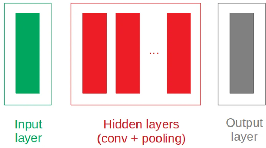
2.1 Commonly used CNN architecture: input layer, combinations of conv and
pooling (hidden) layers and output layer. . . 9
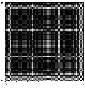
2.2 An example of sensor data represented as an image (GAF). . . 11
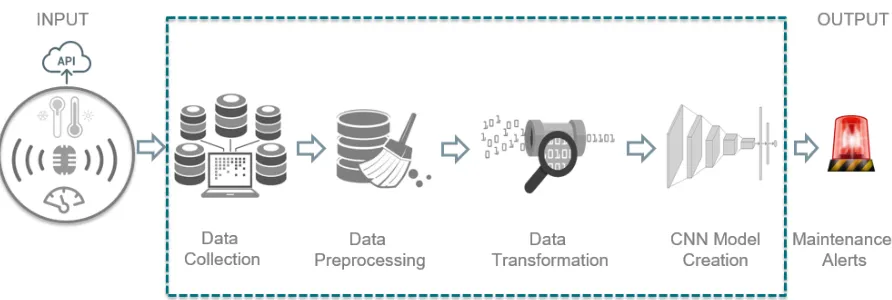
3.1 CNN-PdM framework. . . 20
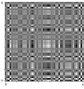
4.1 An example of sensor data represented as an image (multiplication). . . 31
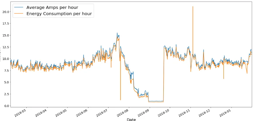
4.2 Amps and energy consumption - SF103B. . . 37
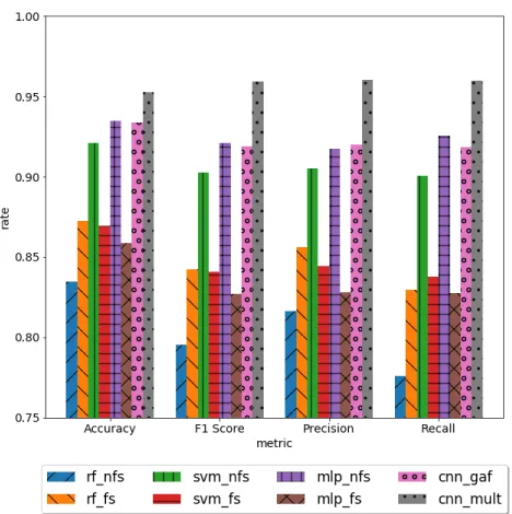
4.3 Comparison among experiments - SF103B (average values). . . 45
4.4 Amps and energy consumption - RF101. . . 49
4.5 Comparison among experiments - RF101 (average values). . . 56
4.1 List of available datapoints. . . 33
4.2 List of available operators. . . 33
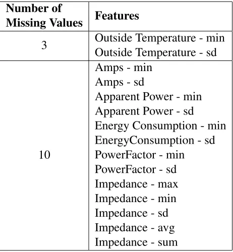
4.3 Number of missing values for each one of the features - SF103B. . . 38
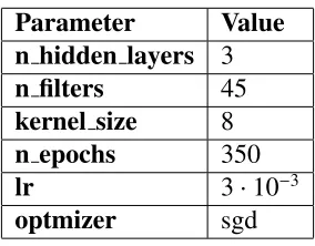
4.4 Parameters for CNN MULT and CNN GAF experiments - SF103B. . . 39
4.5 Parameters for RF NFS experiment - SF103B. . . 41
4.6 Parameters for RF FS experiment - SF103B. . . 41
4.7 Parameters for SVM NFS experiment - SF103B. . . 42
4.8 Parameters for SVM FS experiment - SF103B. . . 42
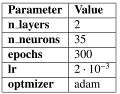
4.9 Parameters for MLP NFS experiment - SF103B. . . 43
4.10 Parameters for MLP FS experiment - SF103B. . . 43
4.11 Metrics comparison among experiments - SF103B (average % values). . . 46
4.12 Metrics comparison among experiments - SF103B (sd % values) . . . 46
4.13 Confusion Matrix for all experiments - SF103B. . . 47
4.14 p-values among experiments - SF103B. . . 48
4.15 Number of missing values for each one of the features - RF101. . . 49
4.16 Parameters for CNN MULT and CNN GAF experiments - RF101. . . 50
4.17 Parameters for RF NFS experiment - RF101. . . 52
4.18 Parameters for RF FS experiment - RF101. . . 52
4.19 Parameters for SVM NFS experiment - RF101. . . 53
4.20 Best parameters for SVM FS experiment - RF101. . . 53
4.21 Parameters for MLP NFS experiment - RF101. . . 54
4.22 Parameters for MLP NFS experiment - RF101. . . 54
4.23 Metrics comparison among experiments - RF101 (average % values). . . 57
4.24 Metrics comparison among experiments - RF101 (sd % values). . . 57
4.25 Confusion Matrix for all experiments - RF101. . . 58
4.26 p-values among experiments - RF101. . . 59
ML Machine Learning
API Application Programming Interface
1-D 1 dimension
2-D 2 dimensions
IoT Internet of Things
CNN Convolutional Neural Networks
ReLU Rectified Linear Unit
SVM Support Vector Machine
RF Random Forest
MLP Multi-Layer Perceptron
conv convolutional
max maximum
min minimum
sd standard deviation
GAF Gramian Angular Field
CNN MULT CNN experiment using multiplication as feature transformation method
CNN GAF CNN experiment using GAF as feature transformation method
RF NFS Random Forest experiment without considering feature selection
RF FS Random Forest experiment considering feature selection
SVM NFS SVM experiment without considering feature selection
SVM FS SVM experiment considering feature selection
MLP NFS MLP experiment without considering feature selection
MLP FS MLP experiment considering feature selection
Chapter 1
Introduction
1.1
Motivation
Nowadays, asset maintenance plays a vital role in companies and countries [1], because, if
an asset breaks, it can cause long downtimes that may affect companies’ production costs or
the comfort level of building occupants. Asset management consumes a large portion of the
budget established by countries and companies. In Canada, the Federation of Canadian
Mu-nicipalities (FCM) has created a five-year, $50 Million program to support muMu-nicipalities to
make decisions on infrastructure investment based on sound asset management practices [2];
Europe reached a record high of EUR 25.2 trillion spent in asset management in 2017 [3].
As-set management is more than just asAs-set maintenance, it considers strategy, safety, environment,
and human factors as well [4]; however, maintenance and terotechnology (ability to maintain
the assets operating optimally) are among the most important competencies for assets
manage-ment, having a substantial impact in a cost perspective [5]. Consequently, a solution that can
improve the handling of asset maintenance can have a considerable impact on the budget of
companies and governments.
There are three main approaches to address the issue of asset maintenance: corrective (also
known as run-to-failure, henceforth R2F) [6]; preventive (or time-based) [7]; and predictive
maintenance (PdM or status based) [8]. In R2F, maintenance only takes place after a failure
occurs. A critical asset failure, such as a broken heating pump in the winter, can lead to
pipes bursting, and may cause severe damage to a building. Preventive maintenance works
under a pre-existing maintenance schedule usually provided by the asset’s manufacturer [7,
9]. The drawback of this approach is that the asset may not present any problem but the
maintenance will be made regardless, resulting in “unnecessary” costs. On the other hand,
PdM performs maintenance based on the asset’s health status indicators. Sensors can measure
an unusual pattern of these indicators, such as an increased motor’s vibration level or higher
energy consumption, and, in most cases, failures are preceded by an unusual pattern of these
measurements [10]. This thesis will investigate the use of PdM in buildings.
In order to apply PdM, two approaches are commonly used: a mathematical model [11] and
machine learning (ML) techniques [8, 10]. A model is a representation of a given phenomenon
or system, which can be made using a set of equations (mathematical) or an ML technique.
A mathematical model usually requires a domain specialist that understands the asset and its
environment. The creation of a mathematical model for an asset is a very specific task; its main
drawback is that the same model cannot be used for different assets. Two distinct mathematical
models had to be created by Bujak [12] and Zhang et al. [13], for example, in order to represent
two different boilers. ML techniques can capture and learn patterns from the data and create
models to evaluate the required health indicators. As buildings have numerous pieces of assets
that must be monitored, the usage of ML is more suitable because it enables the creation of a
specific model for each one of the assets using the same ML techniques.
An important aspect of modeling is to work with the available features. Features are the
different data inputs (individual measurable properties), such as temperature or energy
con-sumption [14]. Dealing with these inputs may be a challenge by itself if two or more highly
correlated features are available because they may introduce bias to the model [14]. The
fea-ture selection step is also significant in order to determine which of the available data inputs are
1.2. Contribution 3
In a scenario in which two different maintenance teams work with the same asset, for instance,
one team may be interested in one set of features and handle only electrical issues with the
asset, while another team may be interested in mechanical features, such as vibration, and be
specialized in mechanical problems.
Different ML techniques perform better under different scenarios. There are ML techniques
that work better with a smaller amount of data, but are outperformed in situations in which the
amount of data drastically increases [15]. Neural Networks (NNs) [16] are one class of ML
techniques that are a combination of cells called neurons, which are organized in layers. The
number of layers of an NN relates to the NN’sdepth. The deeper the NN is, the more layers
(and also neurons) the NN will have. A particular type of NN is the Convolutional Neural
Network (CNN) [15]. The CNNs try to mimic the human brain ability to classify objects by
their shape. For this reason, CNNs are most commonly used for image classification problems.
In other domains, data can be represented as an image through a feature transformation process.
In this research, data transformation methods are used to represent data as images.
1.2
Contribution
This work proposes the Convolutional Neural Network Predictive Maintenance (CNN-PdM)
framework. The CNN-PdM aims at tackling the PdM problem using CNN as its core. The
us-age of CNN is a crucial factor because this technique is capable of creating data representation
from the data’s features, which is a significant advantage when compared to traditional
ma-chine learning techniques as it removes the need to perform feature engineering. Since PdM
is an approach that have the assets’ health status constantly monitored, a drift from normal
behavior indicates that the asset needs maintenance. This study shows that CNN can better
identify abnormal patterns from the data and provide more accurate advice about the need to
perform PdM in assets.
from which CNN can benefit and outperform previous state-of-the-art ML models. More data
represent the possibility to have deeper CNN models, which leads to higher level feature maps
that can be created by the CNN layers; this feature map representation is the main reason why
they outperform conventional ML models as the amount of data increases. A lack of research
in this area suggests that there is no previous usage of Convolutional Neural Networks (CNN)
with electrical data and also in the PdM domain. A data transformation method has also been
proposed to represent 1-dimensional data (1-D) into 2 dimensions (2-D). The multiplication
method, introduced in this research, was able to represent the data in a more heterogeneous
way than the previous data transformation methods; this transformation method combined with
the feature representation from CNNs outperformed conventional ML approaches.
The proposed framework in this thesis was evaluated in two case studies. These case studies
compared CNN-PdM framework using two different image transformation methods and CNN
with well-known ML techniques that have been applied in the PdM domain. For each case
study, one dataset was used for all the experiments. Each one containing data from different
assets (SF103B and RF101) from Claudette MacKay-Lassonde Pavilion (CMLP) building at
Western University, London, Canada. Each dataset contains data from February 1, 2018 to
January 31, 2019.
The results highlight the following observations:
• For comparison purposes, 8 experiments were conducted in this research to assess how
well the CNN-PdM framework would perform when compared with traditional ML
tech-niques used in the PdM domain (Support Vector Machine and Random Forest). Since
CNN is a type of neural network (NN), we are comparing it with Multi-Layer
Percep-tron, which is one of the most commonly used NNs. The evaluation was performed
under 30 simulations for each experiment in two case studies. For each case study, 30
simulations using the same data were performed for each experiment; the CNN
com-bined with the data transformation technique proposed in this work outperformed the
1.3. Organization of theThesis 5
the other approaches by at least 1.91% after, while in the second one, it outperformed the
other approaches by at least 1.5% using also the same data for the experiments.
1.3
Organization of the Thesis
The remainder of this thesis is organized as follows:
• Chapter 2 covers relevant background topics that are necessary to comprehend the
re-maining content of this work. First, this chapter provides information related to machine
learning algorithms used in this work; second, this chapter includes a literature review
on current studies that use CNN for various domains other than image classification and
research that discusses PdM. Finally, it offers distinctions between this thesis and
previ-ously published scholarship.
• Chapter 3 discusses the stages of the CNN-PdM framework, which consists of four
stages: Data Collection, Data Preprocessing, Data Transformation, and CNN Model
Creation. This chapter presents the steps used in each of these stages.
• Chapter 4 describes the implementation performed for the CNN-PdM framework. This
chapter also includes the libraries and methods used for the implementation used in this
research. It also presents the experiments conducted using the CNN-PdM framework
along with a comparison with other ML techniques. Two experiments were performed
that considered two distinct assets: two fans from the CMLP building at Western
Univer-sity that are used for different purposes; therefore, these assets’ electric profile (energy
consumption, amps, real power, and so on) varies from one to another.
• Chapter 5 provides the outcomes of this thesis, as well as discussion regarding Predictive
Background and Literature Review
This chapter has two main objectives: first, it focuses on providing key background information
to help in the understanding of the CNN-PdM framework; second, it presents the literature
review that discusses what has been done on topics related to CNN and PdM.
2.1
Background
This section presents basic concepts of machine learning techniques used in this work:
Con-volutional Neural Networks (CNN), Data Transformation Tecnniques, Random Forest (RF),
Support Vector Machine (SVM), and Multi-Layer Perceptron (MLP). This section also
pro-vides information related to feature transformation and Deep Learning.
2.1.1
Machine Learning
Machine learning (ML) is a field of Artificial Intelligence (AI). ML systems can extract
knowl-edge from data [17] through one of four main learning paradigms: supervised, semi-supervised,
unsupervised, and reinforcement learning [18].
In supervised learning problems, the available data contain the examples (inputs) and also
the target values (outputs), while in semi-supervised problems only a portion of the data
2.1. Background 7
tains the expected outputs. The two most common types of supervised and semi-supervised
learning problems are classification and regression. In classification problems, the ML model’s
output is one of a finite number of classes for a given input. In image classification, one
possi-ble propossi-blem could be, for example, to detect if an object is a cat or not. In this case, it is also
called a binary classification problem, because there are only two possible classes as an output.
Another classic classification example could be to perform the classification of the iris flower
dataset, in which the possible outputs are setosa, virginica or versicolor. This type of problem
is known as a multi-class classification problem. On the other hand, in regression problems,
the ML model’s output is characterized by one or more continuous values. Possible examples
of regression problems are to perform the prediction of energy consumption of an asset for the
next day or to predict Microsoft’s stock value within the next week. To evaluate
classifica-tion problems, some metrics are commonly used, such as accuracy (Equaclassifica-tion 2.1), precision
(Equation 2.2), recall (Equation 2.3) and f1 score (Equation 2.4). These metrics are described
below:
accuracy= 1
nsamples nsamples
X
i=1
(ˆyi =yi) (2.1)
precision= t p
t p+ f p (2.2)
recall= t p
t p+ f n (2.3)
f1 score= 2∗ (precision ∗ recall)
(precision+recall) (2.4)
where ˆyi is the predicted class,yiis the expected class,t pstands for true positives, f pfor false
positives, and f nfor false negatives.
Unsupervised learning is characterized by the absence of labels on the training data.
Clus-tering and density estimation are the most common unsupervised learning problems. ClusClus-tering
is based on the act of grouping examples that share similarities and are usually used as a way
to present insight about the data. Density estimation relates to finding the data distribution in
classes are not provided.
Finally, reinforcement learning relates to unsupervised learning in the sense that ideal
outputs are not provided. The reinforcement learning focuses on finding the optimal output
through a trial and error process. Instead of predicting values, the output of reinforcement
learning techniques is actions. These actions are evaluated by an agent that interacts with the
environment in which it is placed. The evaluation of these actions on the environment works
as a feedback for the model, that can be a reward or a punishment. Volodymyr et al. [19]
presented a reinforcement learning framework that was tested on multiple ATARI games, in
which the pixels from the screen are fed to the agent which learns how to play those games.
Deep Learning is a particular type of ML that presents a unique capability of extracting data
representation. This ability signifies a big step for ML data preprocessing, as a person may not
perform the feature engineering step when using deep learning techniques. Some well-known
deep learning techniques are Convolution Neural Networks, Recurrent Neural Networks, Deep
Belief Network, and Stacked Auto-Encoders [20].
As the name suggests, Machine Learning techniques need to learn (from the data). The
learning stage is called training stage. The data is usually split into two or three subsets:
training, validation (optional), and testing sets. The ML model will learn from the training set,
be affirmed from the validation set, and evaluated within the testing portion of the data. One
could use 80% of the data to train the model and 20% to test (evaluate) it, for instance. This
would be refereed as a 80/20 training/testing data split. Another example would be to have a
validation step. In this case, the data could be split as 60/20/20, that is 60% of the data would
be used to train, 20% to validate, and 20% to test the model.
2.1.2
Convolutional Neural Networks
Deep Learning (DL) is a subset of ML techniques. The main advantage of deep learning
tech-niques is that there is almost no need to perform feature engineering, which is to create features
per-2.1. Background 9
forming representation learning, which means extracting knowledge from raw data. The most
commonly used DL technique for image classification is the Convolutional Neural Network
(CNN).
Inspired by animals’ visual cortex, they have the capability of extracting strong spatially
local correlation to create high-order features information from the raw data [22]. It is possible
to arrange CNN neurons in a three-dimensional structure to capture information regarding
width, height, and depth; therefore, CNNs are commonly used to perform image classification.
CNNs usually present a structured pattern of layers, combining successive convolutional
(conv) layers with ReLU (rectified linear unity as activation function, sometimes seen as a
layer by itself) and pooling layers, represented as a box in the hidden layers stage in Figure
2.1.
Figure 2.1: Commonly used CNN architecture: input layer, combinations of conv and pooling (hidden) layers and output layer.
The convolution operation performed by the convolutional layer is the feature extractor,
which is a filter (also known as a kernel) that slides over data, combining information. Each
filters in the first layer, for instance, would be responsible for detecting the presence of edges,
while the second layer would be in charge of detecting the combination of edges. The third
convolutional layer should be able to detect parts of familiar objects. Note that the abstraction
level increases from layer to layer [21].
The sliding step distance of the filter is known as stride [23]. Usually, the convolution
operation uses stride equals to one, which means that the kernel was shifted by one position.
The output of this filter is the dot product from the filter elements and the data within the kernel
boundaries. This operation can be interpreted as a forced merging of similar features into one
single feature [21].
To avoid overfitting, a very effective technique is used: dropout. A dropout layer is
respon-sible for randomly changing the output of a fraction of neurons to zero, a fraction is known as
dropout rate. An input array [0.1,0.5,0.7,0.3,0.4] submitted to a dropout rate of 0.2 (20%),
for example, would present one of its value set to zero. Dropout is performed only during
the training stage. During testing, the output values are scaled down by a factor equal to the
dropout rate in order to balance the fact that more units are being used than during the training
period.
2.1.3
Data Transformation
As it was previously presented, CNN was created and outperforms conventional machine
learn-ing techniques in image classification problems. Data transformation is a step performed
usu-ally to present data in an easier way to be visualized. A common use of data transformation
is to perform dimensionality reduction, in which large volumes of high-dimensional data are
reduced to 2 or 3-dimensional (2-D and 3-D, respectively) to provide a better understanding of
the data [24, 25]; however, sometimes one needs to perform the opposite task of dimensionality
reduction: to increase the number of dimensions. Mapping the 1-dimensional (1-D) data into
2-D, or even 3-D, is an important step if one considers using a CNN model. Wang and Oates
2.1. Background 11
improving classification and data imputation.
• Grammian Angular Field (GAF): Given the input exampled = {f1, f2, ..., f49}, the GAF
data transformation output can be obtained by applying Equation 2.5:
GAF =
< f1, f1 > · · · < f1, f49>
... ... ...
< f49, f1 > · · · < f49, f49>
(2.5)
where< fi, fj > stands for fi · fj − 2
q
1− fi2· q2
1− fj2. An example of GAF features’
transformation can be seen in Figure 2.2.
Figure 2.2: An example of sensor data represented as an image (GAF).
Chen et al. [27] proposed other two techniques to perform data transformation: Moving
Average Mapping (MAM) and Double Moving Average Mapping (DMAM). For a comparison
purpose, the authors have compared the proposed methods with GAF.
• Moving Average Mapping (MAM):
Moving Average is a well-known technical analysis indicator in the financial domain.
increases the temporal dependency. The authors translated this idea into a mapping
al-gorithm. Their primary goal was to capture multiple moving average values considering
different time frames for each input, as illustrated in Equation 2.6:
MAM=
MAt−D+1,1 · · · MAt,1
... ... ... MAt−D+1,D · · · MAt,D
(2.6)
whereMAi,j is the average stock closing price from periodito j.
• Double Moving Average Mapping (DMAM):
The authors wanted to benefit from more information than only one feature (closing
price) over time. Instead of using the closing price, the authors utilized the average value
from opening and closing prices were used. The aim was that the average value from
opening to closing aggregated more information than only the last one.
MAM and DMAM apply the concept of Moving Average, which represents the variation
over time of a single feature (in DMAM’s case, the average value of two features). Those
techniques are not applicable to the PdM domain when considering different features, such as
energy consumption, amps, or a motor’s vibration level. GAF seems to be the most appropriate
technique to use in the PdM domain. Instead of capturing the correlation among a single feature
over time, it could be used to capture the relationship among features from a specific time; it
is possible to observe, however, that the image representation presented by GAF is dark and
might be a problem, as it presents low contrast among the transformed features (the subtraction
term q2
1− f2 i ·
2
q
1− f2
j decreases the pixel intensity). In order to prevent it, a multiplication
2.1. Background 13
2.1.4
Random Forest
Proposed by Breiman [28], Random Forest (RF) is a technique which creates a set ofNdecision
trees{T1(F),T2(F), ...,TN(F)}, whereF is a feature dimension vector of sizem given byF =
{f1, f2, ..., fm}. Each tree is trained by different subsets of the dataset. Usually, decision trees
are created by splitting each node with the best possible variable, while in RF the node is
split using a subset of features randomly generated for that specific node [29]. This extra
randomness makes RF less prone to overfitting than decision trees. In a classification problem,
the output class is given by the majority vote of the trees in the ensemble, while in a prediction
problem the output is the average value of each tree prediction [30].
2.1.5
Support Vector Machine
Support Vector Machine (SVM) is a commonly used approach in binary classification problems
[8]. Given a training set denoted byS = {xi,yi}ni=1, SVM is responsible for mapping the input
data into a higher dimensional space (greater thann), where it is easier to separate the examples
with a hyperplane [31]; the examples that are closest to the hyperplane are called support
vectors. The hyperplane is surrounded by a margin, which represents how fat this hyperplane
can be without misclassifying the examples; the larger the margin, the better it is, because new
examples can be within the margin without being misclassified.
2.1.6
Multi-Layer Perceptron
Multi-Layer Perceptron (MLP) is a type of feed-forward Neural Network. Its main component,
called neuron, is grouped in layers. Each neuron can receive multiple inputs from the previous
layer, and each input has a weight. The sum of the weighed inputs is modified by a non-linear
function, called activation function. The output of the activation function is used as an input
by the neurons in the subsequent layer. The non-linearity of the activation function allows
hidden and output. MLPs may present more than one hidden layer [22].
2.2
Literature Review
This section provides a literature review and is divided in three parts. The first covers works
in which CNN is used to perform different tasks other than image classification. The second
present works that use mathematical models in the PdM domain, while the last one offers
researches that investigate the creation of ML models in PdM domain.
2.2.1
CNN in Di
ff
erent Domains
CNN was built mostly to perform image classification; however, it has been applied to other
domains [33, 34, 27]. Seo and Cho [33] used CNN to perform offensive sentence classification
as this domain is susceptible to data imbalance. The authors benefited from the transfer learning
capability of CNN and perform its training using an artificial dataset to avoid imbalance issues.
They showed that even though CNN does not perform well in offensive classification as datasets
are usually not enough to train the features (CNN filters), training on an artificial dataset makes
it possible to overcome this issue.
Muckenhirn et al. [34] presented a classification model to deal with voice presentation
attack detection. The authors used a CNN as a feature extractor followed by an MLP with only
one hidden layer that works as a classifier. They concluded that their research is complementary
to a spectral statistics-based approach and its main advantage is that their proposed method does
not use prior assumptions related to speech signals.
Chen et al. [27] proposed a CNN based method to analyze financial time-series. In their
work, they had over one million samples of data from January 2, 2001, to April 24, 2015, and
the sampling period was one minute. The objective of their research was to create a method
that could detect the trend of the time series. The authors used a time-window of size 20 and
Angu-2.2. LiteratureReview 15
lar Field (GAF), Moving Average Mapping (MAM), and Double Moving Average Mapping
(DMAM). The best results were achieved by the combination of GAF and CNN, with an
aver-age of 54.86% accuracy.
2.2.2
Predictive Maintenance using Mathematical Models
Authors have used mathematical models to deal with PdM [11, 35, 36]. Borgiet al. [11]
pro-posed a mathematical model to deal with predictive maintenance for industrial robots. This
method relied on the data analytics of the robot power time-series to predict the robots
ma-nipulator accuracy error. The data used in this work were a set of 21 features (7 for each of
the 3-phase current) and 155 examples. Their work showed that a set of electrical features
presented a high correlation with 3-phase current and the robots accuracy values.
Cauchi et al. [35] presented a mathematical model to describe the user discomfort as a
consequence of degraded temperature control, which advised for maintenance of a boiler. The
authors proposed two models: linear and exponential. The following features were considered
as input for both models: building inside and outside temperatures, boiler efficiency, the ideal
range of comfort temperature, the thermal resistance of the zone envelope, heat gained from
solar radiation, and the heat gained due to occupants. Their methodology aimed to advise for
the boilers maintenance or their replacement.
Olde Keizeret al. [36] offered a mathematical model to tackle problems of systems with
multiple components. The authors demonstrated that the simple fact of duplicating policies
from a single-component into multi-components systems might not be useful. Their
method-ology was based on a Markov Decision Process with a focus on minimizing costs. The model
took into consideration state space, action space, transition probabilities, and the expected
costs. The state space represented the state of each component, status of spare orders and the
number of spare components. The action space represented the decisions made about
compo-nents replacement. The transition probabilities would take into consideration if any component
sum of operating, replacement, order, and holding costs. The results showed that ordering
decisions had a higher impact on the costs than replacement decisions.
The difference between the studies above [11, 35, 36] and the proposed research is that the
CNN-PdM framework uses an ML algorithm; therefore, it is simpler to accommodate different
assets and even asset types than if using a mathematical model. Different ML models can be
trained using the same steps and the same ML technique to work with PdM for a boiler or an
HVAC, for example, while the same mathematical model would not be able to represent both
assets.
2.2.3
Predictive Maintenance using Machine Learning
In contrast with the usage of mathematical models in PdM, machine learning models are also
used [8, 37, 38, 39, 40, 41, 42, 43]. Susto et al. [8] presented an ensemble approach to
detect when tungsten filaments must be replaced during ion implantation, one of the steps
in the semiconductor manufacturing fabrication. The authors had access to 33 maintenance
R2F cycles approach, recording 3671 examples of both normal and faulty data, containing
31 features each (9 for current, 3 for pressure, 7 related with voltage and so on). Susto et
al. tested SVMs ensembles (PdM-SVM) and KNN ensembles (PdM-KNN); the PdM-SVM
slightly outperformed the other approach.
Coradduet al. [37] proposed a study on ML models that performed PdM on gas turbines
(GT). The authors focused on Regularized Least Square (RLS) and SVM to predict the ideal
maintenance time of the GT based on three variables: speed, compressor decay, and GT decay.
The experiments were performed using an artificial dataset created by a simulator. The results
showed that the SVM outperformed the RLS model.
Maet al. [38] presented a Discriminative Deep Belief Network (DDBN) with its
parame-ters optimized using Ant Colony Optimization (ACO) algorithm to deal with predictive
main-tenance on a gas turbine (GT). The authors used 100 different R2F datasets, containing 14
ac-2.2. LiteratureReview 17
cording to their health status into 5 categories, based on how many cycles the GT would work
before it failed: 0%−20%, 20%−40%, 40%−60%, 60%−80%, and 80%−100%. In this study,
the ACO-DDBN model was compared with an ACO-SVM (SVM optimized by ACO) model,
and the ACO-DDBN presented the best results achieving 97% accuracy on the classification
over the 5 classes.
Leahy et al. [39] proposed an SVM approach to perform PdM on wind turbine. The
authors’ dataset was created from SCADA data and presented 45000 datapoints. Leahy et
al. tried to perform 6 different fault classification: fault/no-fault, feeding faults, aircooling
faults, excitation faults, generator heating faults, and mains failure. The authors used SVM
hyperparameter optimization by randomized search. They achieved better results on detecting
generator heating faults, classifying correctly 100% of the cases, but they obtained only 90%
recall and 8% precision on the fault/no fault dataset.
A predictive maintenance for photovoltaic systems using Multi-Layer Perceptron (MLP)
neural network and Triangular Moving Average (TMA) was proposed by De Benedettiet al.
[40]. Their work is based on the prediction of the power generated by the photovoltaic system,
considering the produced power as a function f(I,T), where Iis the solar irradiance and T is
the environment temperature.
Baptista et al. [41] presented a framework that uses data-driven techniques and
Auto-regressive Moving Average (ARMA) to deal with the predictive maintenance for a valve for
an aircraft engine. The feature extraction module uses ARMA to provide a forecast of the next
event. This prediction is used as input for a predictive model in a further step. 13 statistical
features that are created from historical data and are combined with the ARMA’s forecast as a
new set of features. PCA transforms these 14 features, and the output of this transformation is
fed to train the data-driven model. The authors tested f-nearest neighbors, RF, NN, SVMs, and
also linear regression for the data-driven model. The SVM outperformed the other models.
Kulkarniet al. [42] proposed an ML base approach to perform early detection of issues on
consisted of seasonality decomposition and pattern learning by using dynamic time wrapping
and clustering. After that, an RF classifier was used to detect if the pattern was abnormal or
not. Their method was able to achieve 89% precision.
Paolanti et al. [43] presented an ML model to perform PdM on a cutting machine. The
authors used an RF to perform a classification among possible rotor status of the cutting
ma-chine. They had 15 available features and 530731 examples. The authors’ RF model was able
to achieve 95% of overall accuracy.
In contrast with the studies described above [8, 37, 38, 39, 40, 41, 42, 43], the proposed
research makes use of CNN, a model that is capable of extracting feature representation to
outperform classic ML techniques. With a higher number of features, finding an optimal subset
of features can be hard. Only Susto et al. [8] presented a high number of features (31). All
other approaches presented less than 14 features. CNNs are capable of creating relevant feature
representation with a high level of abstraction to perform the classification and in Internet of
Things’ (IoT) era, where more and more data become available every day, being able to deal
with massive amount of features is relevant to any ML problem.
2.3
Summary
This chapter presented an overview of ML models that are key to the understanding of the
CNN-PdM framework, in particular, RF, SVM, MLP, and CNN. Works that use CNN in
do-mains that are not related directly to image classification were also presented in this chapter.
This chapter also presented numerous studies that aim at dealing with PdM by using
Chapter 3
CNN-PdM Framework
This thesis proposes the Convolutional Neural Network Predictive Maintenance (CNN-PdM)
framework, which is presented in Figure 3.1. The CNN-PdM framework uses historical data
gathered by sensors, generates temporal features, performs data transformation, and realizes
model tuning to identify possible degradation of the equipment and advice for maintenance.
The CNN-PdM framework consists of four main stages: the Data Collection, the Data
Preprocessing, the Data Transformation, and the CNN Model Creation. Data transformation
can be seen as a part of the data preprocessing stage, but as the Data Transformation is
partic-ular due to the CNN model, the Data Transformation is represented as a separate stage. The
framework division into these stages makes the CNN-PdM easier to understand as its
respon-sibilities are well defined among each stage. The following sections describe the stages used
in this research.
3.1
Data Collection
This stage presents different sets of data that can be available from an asset. The features can
be categorized asElectrical, such as energy consumption or current;Mechanical, for instance,
vibration or oil level;Contextual and Temporal, which add information about the conditions
(contextual) and time (temporal) in which the asset is working, respectively. When the asset
Figure 3.1: CNN-PdM framework.
performs far from what was expected under those conditions, it becomes possible to detect a
problem. Outside temperature and day of the week provide information about the context in
which the equipment was working in that specific time. Lower energy consumption is expected
from a heating pump during the summer than during the winter, for example.
The data may be acquired by using an API (Application Programming Interface), a SCADA
(Supervisory Control and Data Acquisition) system, or from any other source; sometimes
mul-tiple sources may be used, as contextual features may be collected from external sources, such
as the Historical Climate Data [44], from the Government of Canada. Information such as
temperature, relative humidity, wind speed, and wind direction are available in this domain.
3.2
Data Preprocessing
The preprocessing stage can be divided into multiple steps. This section presents the steps used
in this work.
3.2.1
Dataset Construction
The first step of the data preprocessing is to construct the dataset with all the available data
values from different features. Contextual, electrical, and mechanical features are grouped. If
3.2. DataPreprocessing 21
single dataset is considered as input for the models; therefore, this step is crucial to gather all
available data. The features are grouped by their timestamps to create a matrix that gathers all
the data.
3.2.2
Data Imputation
The next step is to find possible missing values from the previous data matrix. Sometimes,
there are missing values for some features in the data matrix. In this case, the dataset must be
filled for each one of the features. It is essential to be able to fill these values in order to not
discard any available example [45]. Several methods can be used in this step. Two approaches
are more commonly used: to fill the missing values with average, median, or zero, or to use an
interpolation technique, such as linear, time, quadratic, or cubic interpolation.
3.2.3
Feature Creation
At this step, features are created from the timestamps (date and time) information from each
example of the dataset. The Feature Creation step adds temporal information that may be
relevant to the PdM problem. In some scenarios, information regarding the day of the week
or season can add value to the CNN model. The feature creation is also known as feature
engineering. In 2012, Domingos [17] said that “... one of the holy grails of machine learning
is to automate more and more of the feature engineering process.”.
To add temporal information, Equations 3.1 and 3.2 were used to add information regarding
the month, while Equations 3.3 and 3.4 provided knowledge regarding the hours of the day.
month cos=cos
2·π· month
12
(3.1)
month sin= sin
2·π· month
12
hour cos=cos
2·π· hour
24
(3.3)
hour sin= sin
2·π· hour
24
(3.4)
3.2.4
Normalization
The next step is to normalize the data. This step is important to bring every feature to the same
range; depending on the technique used, it is possible to center the data around zero and have
variance in the same order. Some techniques are sensitive to different features ranges (neural
networks, for example). Performing data normalization can make the model less sensitive to
bias. Normalizing the data is the last well-known preprocessing step used in this work.
The two most commonly used techniques to perform data normalization are to scale the
data between an interval (MinMax scaling) or to standardize the data and center it around 0.
The MinMax operation is performed accordingly to the Equation 3.5:
S caled= ei−Emin Emax−Emin
·(max−min)+min (3.5)
where ei is the value to be scaled, Emin is the minimum value for the feature, Emax is the
maximum value for the feature,minis the minimum scale limit (in this research it is -1), and
maxis the maximum scale limit (in this research it is 1). On the other hand, the standard scale
effect is to center the feature in zero and scale it to the unit variance. Equation 3.6 presents how
the standardization process is performed:
S caled= (X−µ)
s (3.6)
where X is the value that is going to be scaled, µis the mean of the samples, and s is their
3.3. DataTransformation 23
3.3
Data Transformation
After the normalization process is completed, the Data Transformation stage begins. CNNs
were created to handle image classification problems; therefore, it is ideal that the data
exam-ples are represented as images.
The data transformation stage is used to represent the single-dimensional (1-D) data (a
fea-ture array) as a two-dimensional (2-D) data (a feafea-ture matrix). This 2-D data can be interpreted
as an image. The goal of an image-like feature representation is to capture the correlation
among features of each specific example from the dataset.
Wang and Oates [26] proposed GAF, a data transformation method, which uses a single
fea-ture during an interval of time. Chenet al. [27] tested GAF and proposed two other methods,
Moving Average Mapping and Double Moving Average Mapping, to perform feature
repre-sentation in financial time-series domain. In Chen’s work, a window would slide over the
same feature through time. The difference between the data transformation performed in their
work and what is proposed in this research is that while in their work the authors captured
the correlation of one feature through time, this research considers one time step only and the
correlation among different features is captured using a data transformation method proposed
in this work: the multiplication method.
3.3.1
The Multiplication Method
The multiplication method was proposed to create more heterogeneous image-like data
repre-sentation than the ones created when using GAF. These heterogeneous patterns in the image
representation can help the creation of different filters by the CNN model, increasing its ability
to correctly classify the data as normal or faulty. Given the example d = {f1, f2, ..., fn}, the
transformed exampleDmis given by a matrix created by the multiplication of the fifeatures by
Dm=
f1· f1 f1· f2 · · · f1· fn
f2· f1 f2· f2 ... f2· fn ... ... ... ... fn· f1 fn· f2 · · · fn· fn
(3.7)
where fi· jj stands for the multiplication of fitimes fj.
3.4
CNN Model Creation
This section presents how the CNN model should be tuned, trained and tested. The tuning
step is important to find the most suitable hyperparameters for the ML problem. The training
should be performed using the hyperparameters found in the previous step. Lastly, the model
should be evaluated in the test step.
3.4.1
CNN Model Parameter Tuning
This step must occur to perform hyperparameter tuning for the CNN model. Different methods,
such as greedy search or randomized search, can be used. In greedy search optimization, all the
possible combinations of hyperparameters for the CNN model are tested, while in randomized
search a randomly generated set of combinations is considered and evaluated. This step is
crucial to obtain an optimized CNN model to handle the PdM problem.
3.4.2
CNN Model Training
As soon as the most suitable hyperparameters are identified, a tuned model is trained. In
real applications, all the available data should be used for training the model. For research
purposes, the data are split to evaluate the model performance. There are different ways to split
the dataset between the training and test sets. Some common ways are 60/40, 70/30, 75/25 or
3.5. Summary 25
shuffling data. The training set should be used in this step to perform the model training, while
the test set should be used to evaluate the model.
3.4.3
CNN Model Testing
The test set generated in the previous step should be used in this step. In this work, the CNN
model is evaluated accordingly to four metrics described in Section 2.1.1: accuracy (Equation
2.1), precision (Equation 2.2), recall (Equation 2.3) and f1 score (Equation 2.4). The confusion
matrix is also generated. Confusion matrix presents information related to the classification
process. This matrix provides information regarding the number fortn, f p, f n, andt p, where:
• tnare negative examples classified correctly (as normal)
• f pare negative examples classified incorrectly (as faulty)
• f nare positive examples (faulty) classified incorrectly (as normal)
• t pare positive examples classified correctly.
In the PdM domain, the worst mistake is to classify a faulty example as normal (f n). If a
datapoint is classified as abnormal, a warning must be created. This notification can be created
and sent out in various ways, such as e-mail, SMS, or even in a dashboard. The a high-level
algorithm of the CNN-PdM framework comprehends steps from the data collection until the
new examples classification. More formally:
3.5
Summary
This chapter has introduced the CNN-PdM framework and discussed each of its core stages:
Data Collection, Data Preprocessing, Data Transformation, and the CNN Model Creation.
The discussion explained the responsibilities of each step and their components, and also how
Algorithm 1:CNN-PdM algorithm.
Data: Hyperparameters (HP), List of Data Sources (DS) Result: Trained Model, Metrics
// Data Collection line 1
1 raw data←collect data(DS);
// Data Preprocessing lines 2-5
2 aggregated data←perform data aggregation(raw data) ; 3 filled data←perform data imputation(aggregated data); 4 completed data←perform feature creation(filled data);
5 normalized data←perform data normalization(completed data);
// Data Transformation line 6
6 transformed data←perform data transformation(normalized data);
// CNN Model Creation lines 7-10
7 training data, testing data←split dataset(transformed data);
8 best hyperparameters←perform hyperparameter tuning(HP, training data); 9 trained model←train model(best hyperparameters, training data);
Chapter 4
Implementation and Evaluation of the
CNN-PdM Framework
This chapter presents the implementation of the CNN-PdM framework. Each section offers a
stage of the framework, the libaries (libs), and methods used in this research. The
implementa-tion of the CNN-PdM framework can be performed for the usage of data from multiple sources.
All the implementation of this work was made using python 3. The following libraries were
used:numpy,pandas,Keras+tensorflow,scikit-learn(sklearn),requests,time, andjson.
This chapter also provides the evaluation of the proposed framework. A description of
the data used in each one of the case studies used in this research and also the evaluation of
the CNN-PdM framework. The data used in this research has been collected in the Claudette
MacKay-Lassonde Pavilion (CMLP) at Western University, London, Canada. The data were
collected by two WebMeters 36F, an accurate equipment able to capture real-time energy data
and which configuration is able to accommodate single, dual, and three phase assets. The
Webmeters were connected to 8 assets from CMLP and their data have been captured. The
installation of these meters was possible because of a partnership between Western
Univer-sity and T-innovation Partners (TiP). TiP provides CircuitMeter devices for measuring various
electricity attributes and CircuitMonitor software which collects data from the meters, stores
them in the cloud, and presents the received data. TiP works with clients to lower their
elec-tricity cost through the use of innovative products for monitoring and controlling of electrical
systems.
The data are derived from two assets: Supply Fan 103B (SF103B) and Return Fan 101
(RF101). These assets were selected because they present very different electrical patterns from
each other. SF103B presents an average energy consumption of 8.31 kW/h and average amps
of 8.67 A, while RF101 presents 0.44 kW/h and 0.54 A average values for energy consumption
and amps, respectively. 1 year of hourly data was collected from February 1, 2018 to January
31, 2019.
4.1
Implementation
This section presents the implementation of the CNN-PdM framework. Details regarding the
libraries (libs) used in each one of the stages and steps are provided in this section.
4.1.1
Data Collection
For this stage, libraries (libs) such asjson, request andtimewere used. The lib requestswas
used to perform multiple API requests. timewas used to sleep the thread for 1 second before
the next request due to an API’s constraint. The result of the request is stored in a json file,
adding also the date of the requested day.
4.1.2
Data Preprocessing
This stage contains 4 steps: Dataset Construction, Data Imputation, Feature Creation, and
4.1. Implementation 29
Dataset Construction
After all the data are gathered in a single file, theDataset Constructionmodule is responsible
for grouping all the features. If external data is used, it must be combined with the asset’s data
by this module. The implementation was made by usingjsonlib to read each line of the file and
convert them into json objects. A parser was created to read each row and create entries into a
pandasdataframe that contained information regarding the measurement name, measurement
value, and date and time (timestamp). The following step was to group the feature values and
name by timestamp.
Data Imputation
TheData Imputationmodule is responsible for filling all the missing values. In this research,
linear interpolation was used in each column to perform this step. Linear interpolation was
used because it is a method accurate enough if the values are closely spaced (which is the
case in this research). Thepandasdataframe object has a methodinterpolatethat was used to
perform the interpolation for each one of the columns using the method ‘linear’.
Feature Creation
In this research, features are created from the timestamp to add temporal information, such as
information regarding the day (if it is a weekday or a weekend), hour, and month. This step is
essential because the temporal features add relevant information, such as seasonality.
To create the information regarding the type of the day (if it is a week-day or weekend
day) from the timestamp, it was only needed to access the date part. Atpandasdataframe, the
datetime object contains information regarding the number of the day of week (0 represents
Monday and 6 Sunday). The information regarding the month (month cos and month sin)
were obtained using the Equations 3.1 and 3.2. The information regarding the hour of the day
(hour cos and hour sin) follows an analogue pattern, shown in Equations 3.3 and 3.4, presented
Normalization
After all the data are together, theNormalizationmodule used theMinMax Scalerto perform
normalization. To do so, thesklearn methodMinMaxScaler was used and the normalization
interval was (-1, 1).
4.1.3
Data Transformation
For the Data Transformation stage, two approaches were tested: Gramian Angular Field
(GAF), presented in Section 2.1.3, and Multiplication, introduced in 3.3.
The feature transformation is performed by using either a method to perform the
multipli-cation of an array by each one of the elements, resulting in a matrix instead of the array or a
method to transform the data using GAF is used. This process is applied to the entire input
dataset by using the methodapply along axisfromnumpylib.
An example of this transformation through multiplication can be seen in Figure 4.1. It is
possible to observe that the subtraction makes the image too dark if one compares the
trans-formation by GAF (Figure 2.2) with the data transformed by multiplication (Figure 4.1). The
problem with a very dark image is that it becomes more homogeneous (more black pixels),
therefore the CNN model is not able to detect the change of pattern in the homogeneous
re-gion. Both images are transformations applied over the same example of the SF103 asset’s
dataset.
4.1.4
CNN Model Creation
This stage contains 3 steps: CNN Model Parameter Tuning, CNN Model Training and CNN
4.1. Implementation 31
Figure 4.1: An example of sensor data represented as an image (multiplication).
CNN Model Parameter Tuning
The CNN Model Parameter Tuning works in the following flow: the dataset is randomly
sampled in a 5-fold cross-validation schema, splitting 80% for training and 20% for testing.
Then the parameters are randomly combined (otherwise it would be an exhaustive search) and
the 5-fold cross-validation sets are used at this step. Accuracy (Eq. 2.1) is the metric used to
evaluate how well a parameter combination performs. This step produces an optimized set of
parameters for the model.
In order to perform the random sampling, the methodtrain test splitfromsklearnis used.
To perform the randomized search, an object of theRandomizedSearchCV class fromsklearn
is created. As the PdM problem, in this case, is considered a classification one and there are
features to capture the seasonality, the data shuffle causes no drawback. This randomized
sam-pling approach was also used by Leathyet al. [39]. As parameters we used keras lib to create
aSequentialmodel using a wrapper fromkerastosklearnlib. This wrapper is responsible for
creating the CNN model using as input a set of hyperparameters (number of layers, number of
kernels, kernel size, number of epochs and so on). TheRandomizedSearchCV object is used
to fit the training test input to the output with a list of possible hyperparameters. After the fit
results.
CNN Model Training
In this research, 30 simulations considering both CNN Model Training and CNN Model
Testing are made for each experiment, considering 80% of the data as training set and the
remaining 20% as testing set, respectively. These sets are randomly sampled from the whole
dataset, and this data split process is repeated for each one of the simulations.
The data are split using thetrain test split method and using the best parameters from the
previous step, the CNN model is created through the wrapper function and the fit method is
used to train the data.
CNN Model Testing
The test set created in the previous step is evaluated in theCNN Model Testingby calculating
four metrics described in Section 3.4.3 and also the confusion matrix. The sklearn lib has a
package with numerous test functions. In this work,accuracy, precision, recall andf1 score
were used. Theconfusion matrixwas also calculated for each experiment.
4.2
Evaluation
This section provides information common to both case studies. The data from both assets
contain the same features. The steps used in both case studies are the ones presented in Chapter
3.
4.2.1
Data Collection
The data are acquired using an API (Application Programming Interface) that has no concept
4.2. Evaluation 33
datapoints collected are described in Table 4.1. With advice from Western’s Facilities
Manage-ment, data from a specific asset (SF103 - Supply Fan 103) have been used in the experiments.
Another asset (RF101 - Return Fan 101) was selected because they offer diverse data;
there-fore, it is important to evaluate if the CNN-PdM framework is able to perform well in both
scenarios.
Table 4.1: List of available datapoints.
Feature Description
Current in A
Energy Consumption in kWh
Power Factor how efficiently the device is working
Outside Humidity %
Outside Temperature in Celcius
Reactive Power power absorbed by a circuit Real Power power dissipated by a circuit Apparent Power sum of reactive and real power
Impedance in ohms
Over the datapoints presented in Table 4.1, it is necessary to apply one of the operators
presented in Table 4.2. These operators are applied according to a given time window. For
this work, the time window was 1 hour. From the combination of datapoints and operators, the
sum of the energy consumption for a given hour, or the maximum value of the current for the
last hour, are examples of possible values that can be requested using the API. For both case
studies, 1 year of data were collected from February 1, 2018 to January 31, 2019.
Table 4.2: List of available operators.
Operator Description
avg Average value
sum Sumation of the values
max Maximum value
min Minimum value
4.2.2
Data Preprocessing
This stage contains 5 steps: Dataset Construction, Data Imputation, Feature Creation, Anomaly
Creation, and Normalization. The importance of this stage is to improve the quality of the data
that will be fed into the CNN models.
Dataset Construction
After all the data are gathered in a single file, theDataset Constructionstep is responsible for
grouping all the features. A parser was created to perform this task. The parser groups all the
features from the previous stage by date and time (timestamp). The output of the parser is a
large matrix containing the timestamp plus the 45 possible features.
Data Imputation
TheData Imputationis performed using linear interpolation to fill the missing values for each
one of the available features. Linear interpolation was used because it is a method accurate
enough if the values are closely spaced (which is the case in this research).
Feature Creation
As soon as the missing values are filled, this step is responsible for using the date (timestamps)
column to create five more contextual features. The timestamp contains two types of
informa-tion: date and time. From the date, it is possible to determine if the example is a weekday or
not. It is also possible to add information about the month of the year (two new features are
generated - sin(month
12 ) and cos( month
12 ), which provide knowledge regarding seasonality. From
the time, two more features are created: sin(hour24 ) andcos(month24 ) [46]. Every feature that uses
sine and cosine to perform a smooth transition from one day to another (in the case of features
created from the hour) or one year to another (in the case of features created from the date).