Exposition on the selection of appropriate experimental design and statistical analysis for pasture improvement research.

(1)

Exposition on the Selection of Appropriate Experimental

Design and Statistical Analysis for Pasture Improvement

Research

W.W. STROUP, S.S. WALLER, AND R.N. GATES

Selection of appropriate treatment and experiment designs are essential elements in research. However, the expense and variabil- ity associated with pasture renovation studio creates unique prob- lems in the application of standard statfstical techniques. Pasture- size renovation studies are restricted by expense, requiring the use of grazing exclosures (subsamples). Treatment design must include an adequate control for treatment comparison. Controls for pas- ture renovation practices cannot be limited to untreated areas within a grazing exclosure. The true measure response is found in the difference between treated areas and a typical grazed pasture situation. Criteria for exclosure selection (homogeneity) and hete- rogeneity of the grazed pasture may result in unequal variances or nonnormal error distributions, thus restricting the use of an analy- sis of variance. The experiment design must recognize the require- ments for making reliable inferences. Pasture-to-pasture variabil- ity generally demands that pastures should be replicated in renovation studies to allow general inferences. Within pasture variability would support the need for multiple exclosures within each pasture. Costs associated with this kind of research limit the utility of idealized experimental designs. Several alternative exper- imental designs are discussed. Limitations in interpretation and risks of drawing erroneous or weak conclusions are reviewed.

Considerable research effort is being expended to develop techniques which will improve forage production in deteriorated areas. Frequently, a major objective of new research is a reduction in the time required for restoration or revegetation. Typical studies often involve intensive examination and data collection from treatments applied to small areas of deteriorated rangeland or pasture fenced to eliminate grazing (exclosure). Such treatments may include chemical application, mechanical disturbance, brush removal, and seeding methods.

Selection of an appropriate experimental design is critical to the success of evaluating treatment effects on pasture. Two major considerations in the development of the experimental design are: experimental treatments must be compared to an appropriate control (treatment design) and the design must provide legitimate replication of the experimental treatments and the control (experiment design). Principles governing the selection of an appropriate design are usually covered in an introductory course in experimental design. However, such a class rarely clarifies the application of

Authors are associate professor, Biometrics and Information Systems Center; professor, Department of Agronomy; and graduate research assistant, Department of Agronomy, University of Nebraska-Lincoln, Lincoln 685834712. Gates is currently assistant professor, Iberia Research Station, Louisiana State University Agricultural Center, Jeanerette 70544.

Published as Paper No. 7736, Journal Series, Nebraska Agricultural Experiment Station.

Manuscript accepted 8 August 1985.

200

these principles to the pasture improvement experiment. Moreover, as Hurlbert (1984) stated: “It is the elementary principles of experimental design, not the advanced or esoteric ones which are most frequently and severely violated by ecologists”.

The objectives of this paper are to: (1) discuss treatment design and appropriate controls, (2) discuss experiment designs and replication, and (3) evaluate several alternatives in experiment design. An example of the data analysis for a typical pasture renovation study is provided.

Selection of the Treatment Design

The ultimate goal of range renovation research is to extrapolate results to pasture situations. An estimate of the difference between predicted performance if renovation were not attempted (e.g., normal management) and that projected if the treatments were applied is of central interest. Ideally, treatments, including an untreated area, would be allocated randomly within each pasture. However, many treatments will have grazing restrictions or recommendations that require nonuse by the grazing animal, restricting any grazing use in such a free-access situation. The lack of grazed, treated areas is unimportant in treatment design, while the lack of a suitable control representing normal management is critical. Most cooperators are not able to remove entire pastures from production while providing others to represent normal management. Consequently, the use of grazing exclosures is an essential element in pasture renovation research. Exclosures also minim- izebndtreatmentcostsandtheriskassociatedwithdetrimentaltreatments.

The grazing exclosure allows the research scientist to screen several potential renovation practices. However, utilization of the ungrazed, untreated area within the exclosure as the “control” presents problems in defining treatment response and the economic value of treatments. The ungrazed, untreated area within an exclosure becomes a unique treatment as a result of the grazing rest, becoming less representative of the grazed pasture with time. This can influence yield as well as species composition data, poten- tially minimizing treatment differences within the exclosure.

Successful treatments may be declared statistically nonsignifi- cant when compared to the ungrazed, untreated area while being extremely successful if compared to the grazed pasture. Relative warm-season grass composition exhibited no difference between an ungrazed, untreated area and an area receiving 1.1 kg/ ha atra- zine (36 and 3770, respectively) at the end of the second growing season. However, the warm-season grass composition was only 14% in the grazed area (T.O. Dill, Department of Agronomy, University of Nebraska, unpublished data). Interpretation of the data could be misleading without the information obtained in the grazed area as well as information on the rate of change of botani-

(2)

cal composition in both the treated and untreated, ungrazed areas. Use of the grazed pasture as a control in range renovation studies presents potential problems in: sampling, replication within the pasture comparable to that in the exclosure, and the potential to have heterogeneous variance compared to the treatments within the exclosure. An exclosure is selected to be as homogeneous as is reasonably possible based upon range site, soil type, vegetation, and topography, while the grazed area is likely to be inherently more heterogeneous. This could result in differential variance due to lack of homogeneity across all treatments. Grazing pattern might also be expected to increase variability of some parameters. Unequal variances restrict the use of conventional analysis of variance (ANOVA) procedures. However, the problems associated with using the grazed area as a control should not detract from the value of establishing adequate economic comparisons for the producer.

The grazed area sampled should be representative of the kind of pasture to which inferences will be made. Consequently, the size of the pasture and the area sampled is not a critical factor. Sampling the grazed pasture should be in areas which are comparable to each exclosure. Generally, areas immediately adjacent to the exclosure should be avoided due to cattle trailing along the fence. However, sampling should occur within close proximity to the general area of the exclosure. Multiple observations within the grazed area must be considered as subsamples. Data collected from the grazed area should be useful in: (1) more accurately assessing the current condition of the area, perhaps documenting seasonal or year-to- year variation, (2) evaluating the degree of success of experimental treatments in changing forage composition and/or yield, and (3) providing comparisons on the speed of recovery due to treatment in contrast to rest without additional treatment. Once appropriate renovation practices are selected from the grazing exclosure trials, trials should be implemented on a pasture size basis to establish the validity of the results and persistence of renovation with grazing.

Selecting the Experiment Design

Selecting an appropriate design for a given experiment includes defining the population (e.g., all native range in eastern Nebraska) to which the conclusions are to be applied, the population of inference. A fundamental precept of the design of experiments is that inference about a population cannot be based upon a single representative of that population. To attempt to do so would fail to insure that the results of the experiment are repeatable, and would not provide the would-be user of the recommendations with an estimate of the magnitude of variability to be expected. The implied population of inference in a pasture renovation study is all pastures to which application of the treatments is contemplated. Therefore a minimum of two pastures (experimental units) randomly selected from the population of inference is an absolute requirement if the results are to have any scientific legitimacy, and more are probably required if the parameters of interest are to be estimated with reasonable precision. Grazing exclosures and observations in the grazed area must be considered subsamples of the experimental unit.

Standard errors are often computed from apparent replications or blocks within an exclosure. This standard error is a measure of the magnitude of variability among plots within the exclosure. If exclosures have not been placed at other positions within the pasture, the experiment provides no evidence that results are reproducible elsewhere in the pasture, much less in other pastures. The estimates of plot-to-plot variability within an exclosure is not an acceptable substitute for more general estimates of variability, within and among the pastures, that are required to extend the scope of inference to the desired population of pastures. This problem has been labelled “pseudo-replication” (Hurlbert 1984). His manuscript is highly recommended for readers desiring a deeper insight into this aspect of design.

JOURNAL OF RANGE MANAGEMENT 39(3), May 1966

Experimental Designs

The

Ideal Design

The “ideal” design for pasture improvement research will be described in this section. It is a design which would thoroughly address all of the considerations presented and allow a statistically tractible and biologically meaningful analysis. It is also a design which, for many researchers, is not practical. Therefore, several alternatives, or compromises will be presented. These alternatives introduce limitations on the scope of inference which are important for the researcher to clearly understand. The effects of these compromises will be discussed.

Model 1

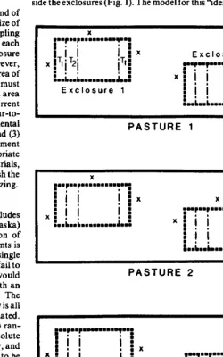
The “ideal”design would utilize several pastures, a minimum of two exclosures per pasture, and grazed control observations outside the exclosures (Fig. 1). The model for this “ideal”design would

X

Exclosure 1

Exclosure r

PASTURE 1

X :..p.p...,..;

ii j i

ix

X

XI

! !

I /

yp.,...,..:

:..b..b...J...

xi

i i

iii

i

5,

5 LA&... . . . . .i..i

PASTURE 2

X

PASTURE P

Fig. 1. An illustration of the “ideal”pasture research design with multiple pastures (1-P). multiple exclosures (l-r) within pastures andsamples (x) of grazed controls “matched”in close proximity to an exclosure. neat- ments (TI-Tt), including an untreated control, are randomly located within an exclosure.

be as follows: T-et yijk denote an observation on the i* pasture, jfi exclosure (or outside observation matched to that exclosure), and k* treatment.

(3)

Then:

yijr = Ir + Pi + e(P)il + tr + (pt)n + (pet)ijk ₍₁₎ where p = overall tnpn

pi = effect of iti pasture (i = 1,2,. ..~ p) e(p)* = ;fyyt ;f j er;closure wnhm 1 pasture

- , ,..*

tk = effect of k treatment (k = 1,2 . . .$,

(pt)ul q e&fect of interaction between the k treatment in the

(pe%ik

i pasture = residual variation

In this situation the grazed control is considered as a true treatment whose effect can be analyzed using an analysis of variance, assum- ing all assumptions for the analysis of variance are met. The only caution regarding this approach is the unbalanced number of samples/ treatment which occurs when the number of observations in the grazed control exceeds the number of exclosures in each pasture.

considered as one source of variation. If the data suggest that

pastures are not a source of variation, a statistician should evaluate the correctness of blocking. Only if blocking was correctly handled should pooling be done when the pasture-by-treatment variance is negligible. Pooling modifies Model 1 to:

yiii = Cc + @)ij + tk + (&X&k

where (pe)~ = effect of ij* exclosure-N(O,+a)

tk = effect k” treatment (pet)* = residual-N(0,0w9

(2)

Tests for treatment effects would then be based upon Ml* (Table 2). It is important to stipulate that Model 2 is a legitimate replace- ment for Model 1 only if 0,: = 0 and at,2 = 0. The principal advantage of Model 2 is increased power due to an increase in the error degrees of freedom from (p-l) (t-l) to (pr-1) (t-l). This increase will be negated if pooling is not appropriate.

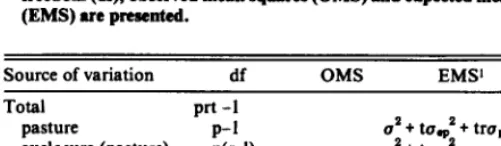
Tebk 1. The ANOVA for the “ideal”d&gn. Source of variation, degreeeof

freedom (at), observed mean squares (OMS) and expected mean square Table 2. The ANOVA for the modifkd ideal design. Source of variation,

(EMS) are presented. degree 01 freedom (df), observed mean equue (OMS) end expected mean

equare (EMS) are presented.

Source of variation df OMS EMS’

Source of variation df OMS EMS’

Total prt -1

pasture _P-l uz + to ’ + tru,’

exclosure (pasture) _p(r-1) a2+ta -2 treatment t-1

pasture X treatment (p-l) (t-l) 2

-2

0’ + rapt + pre, 2 + raB residual p(r-l)(t-1) MI (I*

b% denote random effects as defined above, and 8T denotes that treatments are considered to be fixed effects, since the treatments involved in the experiment are the only treatments of interest.

ANOVA procedures (Table 1) for Model 1 assume that the following are valid characteristics of that data:

1. The model effects pi, e(p)u, tt (pt)n and (pet)bj are mutually independent.

2. Pastures are randomly chosen from a population of pastures whose performance, prior to treatment, would be expected to normally distributed; more formally, each pasture effect is a randomly selected representative from a normal distribution with mean 0 and variance a:. This assumption is denoted symbolically as p,-N(O,a$

3. Consistent with the notation in 2: e(p)ti-N(090y2)

(pt)ti-N(O,+ts) (peth-N(O,u 1.

This ANOVA implies that the proper test for treatment effects is based upon the test statistic (Table 1):

M2

and subsequent mean comparison procedures would use Msas the appopriate error term. This design could also be used to obtain estimates of pasture-by-treatment variance (uti2) and plot-to-plot variance (a’). Plot-to-plot variance (u’) also contains variance due to measurement error. These are useful characterizations of the variability encountered in the experiment and provide information for planning subsequent experiments.

Model 2

If the pasture-by-treatment variance is negligible (Mel), the above analysis can be modified by pooling pasture and exclosure variation. However, caution should be exercised prior to modify- ing the model. While there may be isolated instances in which it is reasonable to assume variability between pastures is negligible, generally it is not. Variances due to blocking criteria can appear negligible because blocks were not sources of variation or because the blocking criteria were mishandled in the experiment. In most range improvement experiments, pastures should be blocks and

Total prt - 1

exclosures pr- 1 up2 + tupez treatments t-1 a~* + pr 8, error (pr-1) (t-l) Zt* us

as’s denote random effects as delined abow, and & denotes that treatments arc considered to be fixed effects, since the treatments involved in the experiment are the only treatments of interest.

Compromises in the Experimental Design

Most researchers will consider the “ideal”design too expensive in terms of resources, manpower, or time to be used without some compromises. Such compromises will normally take the form of one or more of the following:

1. Observe only 1 exclosure per pasture (Fig. 2).

2. Retain replication of exclosures but observe only one pasture (Fig. 3).

3. Replicate by blocking within exclosures, but do not replicate exclosures or pastures (Fig. 4).

These compromises are listed in order of decreasing scientific utility. ‘Compromise l’retains the population of all pastures as the target of inference but sacrifices the ability to estimate within pasture variability. It also provides a legitimate test for the grazed control and only differs from the ideal design in the number of subsamples/experimental unit. ‘Compromise 2’reduces the population of inference to one pasture, and extrapolation must assume that all pastures are alike. This compromise recognizes within pasture variability and allows the researcher to make legitimate statements applicable to the entire pasture. However, since only one pasture is used, there is no legitimate test for the grazed control. ‘Compromise 3’ has the same limitations of ‘Compromise 2’ with the additional loss of an estimate of within pasture variability.

Consider the model and ANOVA corresponding to each compromise (Table 3). Notice that for ‘Compromise 1’ the ANOVA is identical to that implied by Model 1 of the ideal design except for the loss of information about exclosure-toexclosure variability. However, information about the variability among exclosures within pastures is not necessary if the primary objective of the experiment is to draw inferences about anticipated treatment response throughout the population of pastures.

The model for ‘Compromise 2’ is essentially identical to that for ‘Compromise 1’ and to the Model 2 version of the “ideal” design with a single pasture eliminating a test of the grazed, untreated control. However, it remains important to sample the grazed control to characterize existing magnitudes of difference between treatments and “normal management’* (Table 3). The principal

(4)

PASTURE 1

X . . . . “*r.~--““...WT”““!

I

i

!

. x mmm . . . ““.LJ

PASTURE 2

PASTURE P

Fig. 2. An illustration of ‘Compromise I’ in which there are multiple pastures (1-P) with a single exclosure per pasture. Treatments (TI- Td, including an untreated control, are randomly located within the exclo- sure while grazed control observations (x) are made outside the exclosure.

Table 3. Compromise modeb aad ANOVAs.

Exclosure 1

X

:

g..“.;“.“?- . . . .._ “_ :

: i

! i

1

i_i___.“_. ii

. .

X Exclosure r

X

Fig. 3. An illustration of’Compromise 2’in which there is only onepasture with multiple exclosures (l-r) Treatments (TIN, including an untreated control, are randomly located within each exclosure whitkgrased control observations (x) are ma& outside each exclosum.

objection to this design is that it assumes that pasture-to-pasture variability is identical to exclosure-toexclosure variability within a pasture and that relative differences among the treatments are essentially identical for all pastures. There is no provision in this design to examine either of these assumptions. Pasture-to-pasture variation is generally greater than within pasture variability. The risk of using this design is that conclusions based upon a single pasture can misrepresent the true performance in the population of pastures.

Design of a typical pasture improvement pasture improvement experiment involves a single pasture and a single exclosure divided into several blocks, with each treatment and an untreated control being applied once in each block. ‘Compromise 3’ combines a typical experiment with sampling a grazed control (Fig. 4). This design raises a number of statistical difficulties.

Model ANOVA

Compromise 1 (more than I pasture, 1 exclosure per pasture)

SOUrCe df _- EMS

yjj = /A + pi + tj + ptij TOTAL

pi = effect of i” pasture -N(O, oar)

pt-1

tj = effect of j* treatment treatment pasture p-l t-1 o=pt+ ozp

ptu = error-N(O, o*pt) pasture X treatment (error) _{(p-1) 0-f)} + _Qpt+ P@,

Error term for test of treatment effects: MS (pasture X treatment)

Compromise 2 (I pasture, more than 1 exclosure, within exclosure treatments and controls only)

yj = p+ ei + tj + pt)jj

ej = effect of i exclosure -N(O, oz.) tj = effect of j” treatment

(et)ii = error-N(O, os.d

!hKCC df _- EMS

TOTAL rt-1

exclosure r-l ati* + ta2.

treatment t-1 osd + r&

exclosure X treatment (error) (r-l)(t-1) use

Error term for test of treatment effects within pasture: MS(exclosure X treatment)

Compromise 3 (1 pasture, 1 exclosure, within exclosure treatments and controls only)

source df EMS

yu q /A ri + tj + tt)jj TOTAL r(t-1)-l

rj = effect of i block within exclosure blocks r-l

tj = effect of j* treatment

os + (t- l)as*

treatments t-1

(rt)je q effect of ij* block X block X treatment (r-l)(t-2)

a) + r&

treatment combination Error term for test of treatment effects within exclosures: MS(block gtzatment) (asssuming treatment is within exclos-

me)-N(0, a2fi)

(5)

X

X Exclosure

Fig. 4. An illustration of‘Compromise 3’using onepasture, one exclosure.

and observations (x) of the grazed area taken outside of the exclosure. Experimental treatments (TI-Td, including an untreated control. are within the exclosure randomly located within blocks (BI-Bd).

Since it involves exactly one pasture and one exclosure, the analysis of variance is that given (Table 1) with p=l and r=l. Without replicated pastures or multiple exclosures, there are zero degrees of edom in the error terms used to test treatment effects as described earlier. This design may be used to characterize within exclosure treatment effects; however, there is no statistical basis for inference beyond the exclosure unless the withinexclosure variability among ungrazed treatments is identical to pasture-to-pature variability in grazed areas. Since the location of the exclosure is generally seleced for uniformity of soil type, moisture, fertility, etc., this assumption is tenuous. The selection procedure insures that the plots observed are atypically uniform relative to the population, biasing the results.

Data Analysis

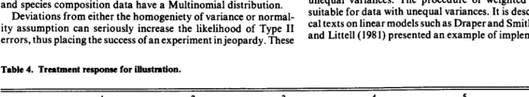
The assumptions required for an ANOVA are that errors are normally distributed and have equal variance for each treatment. The assumption of homogeniety of variance is doubtful when comparing treatments within an exclosure to a grazed treatment outside the exclosure. The assumption of normally distributed errors is, for many response variables, highly suspect. For example, stand counts typically have a Poisson probability distribution, and species composition data have a Multinomial distribution,

Deviations from either the homogeniety of variance or normality assumption can seriously increase the likelihood of Type II errors, thus placing the success of an experiment in jeopardy. These

Table 4. Treatment response for illustration.

problems exist even if the “ideal” design is used; although the “ideal”design also makes the problems easier to clarify and rectify. Cochran (1947) provided a full discussion of the implications of departure from ANOVA assumptions.

Specific methods are required to diagnose departures from ANOVA assumptions and to analyze data using alternative procedures. Diagnosis involves analyzing the experiment using the assumed ANOVA model, calculating the residuals for each observation, and testing them for normality and homogeniety of variance. Specific techniques are given in such statistical texts as Steel and Torrie (1980). Statistical computing packages such as Statisti- cal Analysis Systems (SAS) (Ray 1982) can facilitate analysis of errors (see Example).

If the data fail to satisfy the ANOVA assumptions, the experimenter has four options.

Use a transformation. Guidelines for obtaining a suitable transformation are described in Bartlett (1947) and given in abridged form in such texts as Steel and Torrie (1980). Partition the data into groups of treatments with similar variances and compare these. Pairs of treatments with dissim- ilar variances can be compared using standard paired comparison t-tests. Cochran and Cox (1957) give an example of such a data set partition.

Use a nonparametric procedure. The nonparametric procedure was described by Friedman (1937).

If the variances are unequal and a transformation is not obvious, use weighted least-squares.

Transformations (Option 1) frequently fail in their intended purpose and there are many data sets for which the proper choice of a transformation is not clear. The most useful application of Option 2 is the comparison of the grazed control to other treatments. Observations on the grazed control may commonly have a different variance than observations within the exclosure. The most useful information about the difference between grazed controls and experimental treatments is not a test of whether they are different, but an estimate of how much they are different. Thus, a confidence interval for the magnitude of difference and an economic evaluation of this difference may be the ideal way to address the central objective of the experiment. This would indicate whether the treatment effects are sufficient to justify pasture renovation.

If the structure of the treatment comparison is less obvious, the nonparametric or weighted-least squares (Option 3, 4) are more versatile. For the case of data with homogeneous variances but nonnormal distributions, Conover and Inman (1976, 1981) have shown that the nonparametric procedures generally are more pow- erful than transformation procedures in any event. Friedman’s test (1937) can be implemented using the Conover and Inman rank- transformation procedure. It should be emphasized that nonparametric procedures are not suitable for data known to have unequal variances. The procedure of weighted least-squares is suitable for data with unequal variances. It is described in statistical texts on linear models such as Draper and Smith (198 1). Freund and Littell (198 1) presented an example of implementation of this

Block

1 2 3 4 5 6

1

Herbicide I

Low Level

76 79

E 84 73

2 3 4 5 6

Herbicide 1 Herbicide 2 Herbicide 2 Internal External

High Level Low Level High Level Control Control

88 86 90 73 76

81 77 82 69 67

85 79 87 74 42

90 85 91 16 59

90 87 100 84 21

84 84 83 70 68

(6)

procedure using SAS.

Example

Consider an experiment conducted using the randomized block design in ‘Compromise 1’. In this particular design pastures are the blocks. This design has been selected for illustration of the various analytical methods detailed in this paper because it is considered to be the most statistically desirable, “practical” design. Suppose the experimenter wishes to test the effect of 2 herbicides at 2 rates plus an internal untreated control (grazing rest) and an external grazed control. The treatment design is a 2 X 2 factorial plus 2 controls. Specific experiments will use different treatment designs; this design is used because it is both relatively simple and typical.

This example will consist of 3 sections: (1) the data set and its preliminary characterization, (2) the ANOVA under standard assumptions, and (3) analysis using transformations with nonparametric methods. Since many researchers use SAS, appropriate examples will be given for the program statements.

Preliminary Characterization

of

the Data

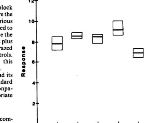
The data for this illustration are given (Table 4). Prior to computing a formal statistical analysis of these data, the researcher should do a preliminary characterization of the data. A particularly helpful technique, suggested by Tukey (1977), is a box-plot. A box-plot is obtained by computing the median and first-and-third quartiles of the data for each treatment and arranging them side- by-side, as illustrated (Fig. 5). This particular side-by-side box-plot should alert the researcher to four important features of these data: (1) within each herbicide the response seems to increase with increased herbicide level; (2) these increases are consistent for each herbicide type; (3) the controls, particularly the external control, have characteristically lower response than the treatments; and (4) the external control exhibits sharply greater within-treatment variation than any of the treatments within the exclosure. This fourth point should be pursued prior to a formal analysis of the data since it indicates that the assumption of equal variances for each treatment is not valid.

third

El

l__l fht auartlh

Fig. 5. Box plots for the treatments used in the example of a herbicide study with 2 herbicides at 2 rates (I-4)plus an internal untreatedcontrol (5) and an external control (4).

The degree to which the data conform to the ANOVAassump- tions can be tested in the following manner:

1) Compute the mean for each pasture, for each treatment, and for the entire data set. Denote these yi, Fj, and F.., respectively. 2) Estimate the effect of each pasture by calculating pi= Fi.- y. .

for each level of i.

3) Estimate the effect of treatment by tj = y.j -7. . for each level of 1.

4) Calculate the estimated error for each observation by the

Table 5. SAS program and s&&d output to e&mate and examine conformity of errors to ANOVA aesumptions.

PROGRAM DATA A; INFILE IN;

INPUT PASTURE TRT Y;

PROC GLM; CLASSES PASTURE TRT, MODEL Y=PASTURE TRT;

OUPUT OUT=B RESIDUAL=RES_Y; PROC SORT; BY TRT;

PROC UNIVARIATE NORMAL PLOT; BY TRT; VAR RES_Y;

OUTPUT TRT=l, UNIVARIATE; VARIABLES=RES_Y MOMENTS

N 6

MEAN 5.921E-15 STD DEV 5.46938 SKEWNESS 0.351029

uss 149.079

cv 9.222E+16 T:MEAN=O 2.656E-15 SGN RANK 0.5 NUM -= 0 6 W:NORMAL 0.871907

SUM WGTS SUM VARIANCE KURTOSIS css STD MEAN PROB>]TJ PROB>]S]

PROBCW

QUANTILES (DEF=4)

6 100% MAX 7.13889 99% 7.13889 3.553E-14 75% 43 5.76389 95% 7.13889

29.8157 50% MED -1.19444 96% 7.13889

-2.30185 25%

Ql

-4.77778 10% -5.52778 149.079 0% MIN -5.52778 5% -5.52778

2.22919 1% -5.52778

1 RANGE 12.6667

1

43-41

10.5417

MODE -5.52778 0.281

EXTREMES

LOWEST HIGHEST -5.52778 -4.52778 4.52778 -4.02778 -4.02778 1.63889

1.63889 5.30556 5.30556 7.13889

(7)

fOlTllllh: eij = yij - (7. . + pi + tj).

Note this equation follows directly from the model equation (1).

5) Calculate the variance among the errors for each treatment. Note there should be one variance calculated for each treatment. These can be examined for equality.

Steps 1 and 4 above can be implemented with SAS using the

Tabk 7. SAS propua and aekcted output for slmdard malysk.

PROGRAM:’

DATA A; INFILE IN;

steps illustrated (Table 5). Sample output is given for treatment 1. The items of interest in this output are the “VARIANCE”and the “W:NORMAL”and its associated significance level “PROB<W.” The former can be used to evaluate equality of the variances for the various treatments. The latter tests for the normality of the errors. Without going into the theory of the test for normality, it is sufficient for the researcher to know that low values of W:NOR- MAL are associated with nonnormal data; PROB<W is the probability that a lesser value of WNORMAL would occur by chance alone if the data are in reality normally distributed. Thus it can be interpreted exactly as any other significance level: low PROB<W implies nonnormal data; high PROB<W implies normal data.

INPUT PASTURE TRT Y;

PROC GLM; CLASSES PASTURE TRT; MODEL Y=PASTURE TRT,

MEANS TRT,

CONTRAST HERBICIDE’TRT 1 I -1 -1 0 0; CONTRAST ‘LEVEL’TRT 1 -1 1 -1 0 0; CONTRAST ‘H BY L’TRT 1 -1 -1 1 0 0;

CONTRAST ‘HERB’VS CTL’TRT-1 -I -1 -I 2 2; CONTRAST ‘IN-Cl-L VS OUT-CTL’ TRTO 0 0 0 1 -1;

MEAN SQUARE 476.49444444

85.54777778 A full summary of the results of the test for normality and the

variances among the errors for each treatment is given (Table 6).

OUTPUT: DEPENDENT VARIABLE Y SUM OF SOURCE DF SQUARES

MODEL 10 4764.94444444

ERROR 25 2138.69444444

CORRECTED TOTAL 35 6903.63888889

Tabk 6. Summary of nomutity and varimce resulta for data.

MODEL F = 5.57

R-SQUARE cv ROOT MSE

0.690208 11.8117 9.24920417

PR>F = O.OQQ2 Y MEAN 78.305555556

Treatment PROB<W Variance

:

.207 31.17

.251 8.57

3 569 8.06

4 .373 36.01

5 .Q47’ 32.44

6 .2% 313.832

lTreatment 5 fails to satisfy the assumption of normally distributed errors. Treatment 6 StCms to have highly inflated variance relative to other treatments observed within the exclosum (treatments 1 through 5).

SOURCE DF TYPE I SS

PASTURE 5 403.13888889

TRT 5 4361.80555556

SOURCE DF TYPE III SS

PASTURE 5 403.13888889 TRT 5 4361.80555556

CONTRAST DF ss

HERBICIDE 1 146.16666667 LEVEL 1 266.66666667 HBYL 1 10.66666667 HERB VS CTL 1 2999.22222222

IN-CTL VS OUT-Cl-L I 954.08333333

F VALUE 0.94 10.20 F VALUE 0.94 10.20 PR>F 0.4710 0.0001 PR>F 0.4710 0.0001

F VALUE PR>F

1.64 0.2123

3.12 0.0897

0.12 0.7270

34.95 0.0001

11.15 0.0026

The information for the variances seems to confirm the pictorial implication of the box-plots that the assumption of homogeneity of variance is not satisfied. Moreover, the assumption of normality does not appear to hold for one of the treatments. It should be noted that the power of this test of normality, based upon minimal observations, is low. Only extreme departure from normality will lead to a conclusion that the data are nonnormal. In addition, any test will produce sporadic rejections of the null hypothesis. An isolated instance of a low PROB<W does not necessarily suggest data for that treatment are nonnormal; it may be indicative of a Type I error. However, it could reflect a problem in the execution of the experiment leading to a deviant set of observations. Thus an unusually low PROB<W should alert the researcher to review the data.

‘Null hy othcses tested by contrasts are: I) means of herbicide 1 and 2 arc equal, 2) means o P herblclde levels are eoual. 3) no herbicide bv level interaction. 4) mean of ” controls and mean of herbicide tk&&nts are equal, aid 5) mean of intekicontrol is equal to external control.

the chance of Type II errors. Peterson (1977) and Little (1978) addressed the misuse of multiple range tests.

In this example, the principal features of the data are most clearly revealed by orthogonal contrasts. The SAS program statements and resulting analysis are presented (Table 7). Alternatively, if the objective of the experiment is to compare each experimental treatment with the ungrazed control, Dunnett’s test (Steele and Torrie 1980) is appropriate. Confidence intervals may be computed for differences which are significant and these may be used for subsequent costeffectiveness evaluation.

Standard Analysis of the Data Conclusion

The diagnostic tests (for normality and equality of variance) should be standard procedure for all data sets. These tests indi- cated that the data in this illustration do not satisfy the assumptions of ANOVA. Therefore, in practice, the researcher and consulting statistician should proceed with alternative analyses consistent with the data and objectives of the study. However, researchers will often encounter data sets which comply with the assumptions of ANOVA; consequently, a standard analyses will be presented to illustrate SAS programming and possible mean comparisons.

The basic ANOVA follows from the randomized complete block (pasture) model. The SAS statements required to obtain this analysis are presented (Table 7). Many researchers generally perform a multiple range test, e.g., Duncan’s multiple range test or Student- Newman-Keuls. However, multiple comparison tests are inevita- bly less revealing of the principal features of the data than are other procedures more directly connected to the objectives of the experiment. In addition, multiple comparison tests generally increase

Design and analysis of pasture experiments needs careful atten- tion. Consideration of the population of inference should be used in selecting experimental pastures. Replication of pastures is essential for adequate treatment evaluation and inference. An appropriate control is an important and presently overlooked aspect of treatment design. Grazed controls outside the exclosure will greatly aid the researcher in assessing the effectiveness of treatments. Selection of an appropriate experimental design cannot be overemphasized. Standard ANOVA methods are not always appropriate due to the nature of the data obtained from pasture experiments. Many response variables commonly of interest to the range scientist do not conform to the assumptions underlying the ANOVA. If the data do not adhere to the basic assumptions associated with ANOVA, the researcher must be prepared to utilize alternative methods of data analysis. Nonparametric methods seem particularly promising for comparative experiments conducted in this area.

(8)

Litenture

Cited

Bmtktt, M.S. 1947. The use of transformations. Biometrics 3:39-52.

Cochran, W.G. 1947. Some consequences when the assumptions for the analysis of variance are not satisfied. Biometrics 3:22-38.

Co&ran, W.G., and Cox, G.M. 1957. Experimental designs, 2nd ed. John Wiley & Sons, New York.

Conover, W.J., and R.L. Iman. 1976. On some alternative procedures using ranks for the analysis of experimental designs. Commun. in Statis- tics, Seri. A5:1348-1368.

Conover, W.J., and R.L. Iman. 19Il1. Rank transformations as a bridge between parametric and nonparametric statistics. Amer. Statistician 35124-128.

Draper, N.R.,snd H. Smith. 1981. Applied regression analysis. John Wiley and Sons, Inc. N.Y.

Friedman, M. 1937. The use of ranks to avoid the assumption of normality implicit in the analysis of variance. J. Amer. Statis. Ass. 32:675-701.

Freund, R.J., and R. L&tell. 1981. SAS for linear models. SAS Institute. Cary, N.C.

Hurlbert, S.A. 19g4. Pseudoreplication and the design of ecological field experiments. Ecol. Monog. 54: 187-211.

LIffle, T.M. 1978. If Galileo published in HortScience. Hort-Sci. 13504-506. Petenon, R.G. 1977. Use and misuse of multiple comparison procedures.

Agron. J. 69205~208.

Ray, A.A. ed. 1982. SAS user’s guide. SAS Institute, Cary N.C. Satterthwaite, F.E. 1946. An approximate distribution of estimates of

variance components. Biom. Bull. 21 IO-1 14.

Steel, R.D.G., and J.H. TorrIe. 1980. Principles and procedures of statistics: a biometrical approach. McGraw-Hill, New York.