Twisted Jacobi Intersections Curves
Rongquan Feng
1, Menglong Nie
1, Hongfeng Wu
21LMAM, School of Mathematical Sciences, Peking University,
Beijing 100871, P.R. China
2Academy of Mathematics and Systems Science, Chinese Academy of Sciences,
Beijing 100190, P.R. China
[email protected], [email protected], [email protected]
Abstract
In this paper, the twisted Jacobi intersections which contains Ja-cobi intersections as a special case is introduced. We show that every elliptic curve over the prime field with three points of order 2 is iso-morphic to a twisted Jacobi intersections curve. Some fast explicit for-mulae for twisted Jacobi intersections curves in projective coordinates are presented. These explicit formulae for addition and doubling are almost as fast as the Jacobi intersections. In addition, the scalar mul-tiplication can be more effective in twisted Jacobi intersections than in Jacobi intersections. Moreover, we propose new addition formulae which are independent of parameters of curves and more effective in reality than the previous formulae in the literature.
Keywords: elliptic curves, Jacobi intersections, twisted Jacobi intersec-tions, scalar multiplication, isomorphic
1
Introduction
important role in the efficiency of the whole system. Elliptic curves can be represented in different forms. To obtain faster scalar multiplications, several elliptic curve representations have been considered in the last two decades. The detail of previous works can be find in [1, 3, 7].
Jacobi intersections curve is the intersection of two quadratic surfaces in three dimensional space with a point on it. The scalar multiplication on Jacobi intersections show competitive efficiency in scalar multiplication, such as faster doubling and tripling operations. Chudnovsky and Chudnovsky [5] proposed first fast doubling and addition formulae for Jacobi intersections in projective coordinates. Liardet and Smart [8], and [1] presented slightly faster formulae. Hisil etc. [6] presented faster tripling formulae. Some slightly faster formulae with a trick can also be found in [7].
In this paper, the Jacobi intersections is generalized to “twisted Jacobi intersections” which contains Jacobi intersections as a special case. It is show that every elliptic curve over the prime field with three points of order 2 is isomorphic to a twisted Jacobi intersections curve. Some fast explicit formulae for twisted Jacobi intersections curves in projective coordinates are presented. These explicit formulae for addition and doubling are almost as fast in the general case as they are for the Jacobi intersections. In addition, the scalar multiplication can be more effective in twisted Jacobi intersections than in Jacobi intersections. Moreover, we propose new addition formulae which are independent of parameters of curves and more effective in reality than the previous formulae in the literature.
2
Jacobi intersections and Twisted Jacobi
In-tersections
In this section we briefly review Jacobi intersections curves and the Jacobi intersections addition law. We then introduce twisted Jacobi intersections curves and discuss their relations to Jacobi intersections curves.
Jacobi intersections.
Throughout the paper we consider elliptic curves over a non-binary field
K, i.e., a fieldK whose characteristic is not 2.
A Jacobi intersection form elliptic curve overK is defined by
u2+v2 = 1
bu2+w2 = 1,
where b ∈ K with b(1−b) 6= 0. A point (u, v, w) on a Jacobi intersections curve is represented as (U :V :W :Z) satisfying
U2+V2 =Z2, bU2+W2 =Z2
and (u, v, w) = (U/Z, V /Z, W/Z). Here (U :V :W :Z) = (λU :λV :λW :
λZ) for any nonzero λ ∈ K. The negative of (U : V : W : Z) is (−U : V :
W : Z). The neutral element (0,1,1) is represented as (0 : 1 : 1 : 1). The reader is refereed to [5] for more details on Jacobi intersections curves.
The affine version of the unified addition formulae, i.e., that can han-dle generic doubling, simplifying protection against side-channel attacks, are given by
(u3, v3, w3) = (u1, v1, w1) + (u2, v2, w2),
where
u3 =
u1v2w2+u2v1w1
v2
2+u22w21
, v3 =
v1v2 −u1w1u2w2
v2
2+u22w21
, w3 =
w1w2−bu1v1u2v2
v2
2+u22w21
.
The point addition formulae in projective homogenous coordinates are given by
(U3 :V3 :W3 :Z3) = (U1 :V1 :W1 :Z1) + (U2 :V2 :W2 :Z2),
where
U3 = U1Z1V2W2+V1W1U2Z2, V3 =V1Z1V2Z2−U1W1U2W2
Twisted Jacobi Intersections.
Definition 1. A twisted Jacobi intersection form elliptic curve over K is defined by
au2 +v2 = 1
bu2+w2 = 1,
where a, b ∈ K with ab(a−b) 6= 0. A Jacobi intersection elliptic curve is a twisted Jacobi intersection curve with a= 1.
The twisted Jacobi intersection curveEa,b: au2+v2 = 1, bu2+w2 = 1 is a
quadratic twist of the Jacobi intersection curveE1,b/a : ¯u2+¯v2 = 1, (b/a)¯u2+
¯
w2 = 1. The map (u, v, w) 7→ (¯u/√a,v,¯ w¯) is an isomorphism from E
a,b to
E1,b/aoverK(
√
a). Thus ifais a square inKthenEa,bis isomorphic toE1,b/a
overK. More generally,Ea,bis a quadratic twist ofE¯a,¯b for any ¯a,¯bsatisfying
¯
b/¯a=b/a. Conversely, every quadratic twist of a twisted Jacobi intersection curve is isomorphic to a twisted Jacobi intersection curve, i.e., the set of isomorphism classes of twisted Jacobi intersection curves is invariant under quadratic twists.
Every twisted Jacobi intersection curveEa,b: au2+v2 = 1, bu2+w2 = 1
is birationally equivalent to a Jacobi quartic elliptic curve E4,,δ : y2 =
x4+ 2δx2+ 1 with = 1/a2, δ = (a−2b)/a2 under the transformations
x = (v−1)/u,
y = w(a+x2)/a, and
w = ay
a+x2,
u = (w
2−1)(a+x2)
2bx ,
v = 1 +xu.
Theorem 1. Let K be a field with char(K) 6= 2 and Ea,b : au2 +v2 =
1, bu2+w2 = 1 be a twisted Jacobi intersection form curve define over K
withab(a−b)6= 0. ThenEa,b is a smooth curve and isomorphic to an elliptic
curve of the form E :y2 =x(x−a)(x−b) overK.
Proof. The proof is given in Appendix.
Proof. LetE be an elliptic curve over K having three K−rational points of order 2. Let (θ1,0),(θ2,0) and (θ3,0) be these three distinct points of order
2 on the Weierstrass curve E, i.e., y2 =x3+a2x2+a4x+a6 = (x−θ1)(x−
θ2)(x−θ3). Replacing (x, y) by (x+θ1, y) yields the equation of the form
y2 =x(x−a)(x−b), where a=θ
2−θ1, b =θ3−θ1. Therefore every elliptic
curve over K having three K−rational points of order 2 is isomorphic to a twisted Jacobi intersections curve by Theorem 1.
3
Arithmetic on Twisted Jacobi Intersections
LetK be a non-binary field. In this section we present fast explicit formulae for addition and doubling on twisted Jacobi intersections curves over K.
Theorem 3. LetP = (u1, v1, w1), Q= (u2, v2, w2)be two points on a twisted
Jacobi intersections elliptic curve Ea,b : au2+v2 = 1, bu2+w2 = 1, and let
R = P +Q := (u3, v3, w3). Then the affine version of the unified addition
formulae are given by
u3 =
u1v2w2+u2v1w1
v2
2 +au22w12
, v3 =
v1v2−au1w1u2w2
v2
2 +au22w12
, w3 =
w1w2−bu1v1u2v2
v2
2 +au22w12
.
Especially, if P =Q and R= 2P := (u3, v3, w3), then
u3 =
2u1v1w1
v2
1+au21w21
, v3 =
v2
1−au21w12
v2
1 +au21w12
, w3 =
w2
1 −bu21v21
v2
1 +au21w21
.
The identity element is(0,1,1). The negative of the point(u, v, w)is(−u, v, w).
Proof. For the correctness of the addition law, observe that it coincides with the Jacobi intersections addition law on
¯
u2+v2 = 1, b au¯
2+w2 = 1,
with ¯u=√au. These formulae also work for doubling.
Theorem 4. Let K be a field of odd characteristic. Let Ea,b : au2 +v2 =
1, bu2 +w2 = 1 be a twisted Jacobi intersections curve over K. Let P =
(u1, v1, w1) and Q = (u2, v2, w2) be points on Ea,b. If ab is not a square in
K, or if −1 is a square in K and neither a nor b is a square in K, then
v2
Proof. If v = w = 0, then au2 = bu2 and a = b, therefore ab is a square
in K, contradict to ab is not a square in K. Therefore at most one in
{u, v, w} is equal to 0 for a point (u, v, w) on Ea,b. Thus if u2 = 0, then
v2
2+au22w12 =v22 6= 0. Ifu1 = 0, thenw12 = 1, andv22+au22w12 =v22+au22 = 1.
Let u1u2 6= 0, assume that abis not a square in K. If v22+au22w12 = 0, then
au22 +v22−(v22 +au22w21) = au22(1−w21) = 1. Thus 1−w12 = 1/au22 = bu21. thereforeab= (1/u1u2)2 is a square inK, contradict to the assumption. Now
assume that neitheranorbis a square inK, thenw1v2 = 0. If6 v22+au22w12 = 0,
then a =−(v2/u2w1)2 is square inK since −1 is a square in K, which is a
contradiction.
Note that the Theorem 4 shows that if ab is not a square in K, then the twisted addition formulae is complete. But generally, both a and b are non-squares in K. Therefore ab is not a square in K is not a reasonable assumption when a 6= 1. But in this case, if −1 is a square in K, then the above twisted addition formulae is also complete.
When using projective homogenous coordinates to eliminate field inver-sions, each point is represented by the quadruplet (U : V : W : Z) which satisfies the equations
aU2+V2 =Z2, bU2+W2 =Z2,
and corresponds to the affine point (U/Z, V /Z, W/Z) withZ 6= 0.
Theorem 5. Let P = (U1 : V1 : W1 : Z1), Q = (U2 : V2 : W2 : Z2) be two
points on the twisted Jacobi intersections elliptic curve Ea,b : aU2 +V2 =
Z2, bU2+W2 = Z2, and let R = P +Q := (U
3 : V3 : W3 : Z3). Then the
projective version of the unified addition formulae are given by
U3 = U1Z1V2W2+V1W1U2Z2, V3 =V1Z1V2Z2−aU1W1U2W2,
W3 = W1Z1W2Z2−bU1V1U2V2, Z3 =Z12V22+aU22W12.
The identity element is (0 : 1 : 1 : 1). The negative of the point (U : V :
W :Z) is(−U :V :W :Z).
Note that Z12(Z22 −V22) = aZ12U22 and aU22(bU12 +W12) = aU22Z12. We have Z2
1V22 +aU22W12 = Z12Z22 −abU12U22 which can be used to simplify the
Especially, the above theorem gives the following doubling formulae.
U3 = 2U1V1W1Z1, V3 =V12Z12−aU12W12,
W3 = W12Z12−bU12V12, Z3 =V12Z12+aU12W12.
Note thatbU12 =Z12−W12, andV12W12 =W12(Z12−aU12) =W12Z12−aU12W12. We have the second doubling formulae
U3 = 2U1V1W1Z1, V3 =V12Z12−aU12W12,
W3 = 2W12Z12−V12Z12 −aU12W12,
Z3 = V12Z12+aU12W12.
(1)
Moreover, from
W12Z12−bU12V12 = W12(aU12+V12)−(Z12−W12)V12 =aU12W12+ 2V12W12−V12Z12
= aU2
1W12 −V12Z12+ 2W12(bU12+W12 −aU12)
= aU2
1W12 −V12Z12+ 2bW12U12+ 2W14 −2aU12W12
= −aU12W12−V12Z12+ 2(bU12W12+W14),
we have the third doubling formulae
U3 = 2U1V1W1Z1, V3 =V12Z12−aU12W12,
W3 = −aU12W12−V12Z12 + 2(bU12W12+W14),
Z3 = V12Z12+aU12W12.
(2)
Addition in Projective Coordinates. By Theorem 5, the following for-mulae compute (U3 :V3 :W3 :Z3) = (U1 :V1 :W1 :Z1) + (U2 :V2 :W2 :Z2)
denote the two algorithms by ”AProjective.1” and ”AProjective.2”.
A = U1V1; B =W1Z1; C=U2V2; D=W2Z2; E =U1W2;
F = V1Z2; G=W1U2; H =Z1V2; J =AD; K =BC;
U3 = (H+F)(E+G)−J −K;
V3 = (H+E)(F −aG)−J+aK;
W3 = (B−bA)(C+D) +bJ −K;
Z3 = H2+a·G2 =H2+aG·G.
If the points represented by the sextuplet (U, V, W, Z, U V, W Z), then the addition formula can by modified by: (U3 : V3 : W3 : Z3 : A3 : B3) =
(U1 : V1 : W1 : Z1 : A1 : B1) + (U2 : V2 : W2 : Z2 : A2 : B2), where
A1 =U1V1, B1 =W1Z1, A2 =U2V2, B2 =W2Z2. The cost are 11M+ 2S+ 5D
or 12M +S+ 4D. We denote the two algorithms bye ”MProjective.1” and ”MProjective.2”.
C = U1W2;D=V1Z2;E =W1U2;F =Z1V2;G=A1B2;H=B1A2;
U3 = (D+F)(C+E)−G−H;
V3 = (C+F)(D−aE)−G+aH;
W3 = (B1−bA1)(A2+B2) +bG−H;
Z3 = F2+a·E2 =F2+aE·E;
A3 = U3V3;B3 =W3Z3.
Note that, if a=ε2 is a square element in the field, thenZ
3 = (F +εE)2−
2εH, the cost is 11M+ 1S+ 6D.
Doubling 1 in Projective Coordinates. The following formulae compute (U3 :V3 :W3 :Z3) = 2(U1 :V1 :W1 :Z1) in 3M+ 4S+ 1D by using formulae
(1), where the 1D is a multiplication by a:
A = V1Z1; B =A2; C =U1W1; D=C2; E = 2(W1Z1)2;
U3 = (A+C)2−B−D; V3 =B −aD;
W3 = E−B−aD; Z3 =B+aD.
Doubling 2 in Projective Coordinates. The following formulae compute (U3 :V3 :W3 :Z3) = 2(U1 :V1 :W1 :Z1) in 2M+ 5S+ 2D by using formulae
(2), where the 2D are multiplications by a and by b:
A = V1Z1; B =A2; C =U1W1; D=C2; E =W14;
U3 = (A+C)2−B−D; V3 =B−aD;
Doubling 1 in Projective Coordinates with Z1 = 1. The following
formulae compute (U3 :V3 :W3 :Z3) = 2(U1 :V1 :W1 : 1) in 1M + 4S+ 1D
by using formulae (1), where the 1D is a multiplication by a:
A = V1; B =A2; C =U1W1; D=C2; E = 2W12;
U3 = (A+C)2−B−D; V3 =B−aD;
W3 = E−B −aD; Z3 =B +aD.
Doubling 2 in Projective Coordinates with Z1 = 1. The following
formulae compute (U3 :V3 :W3 :Z3) = 2(U1 :V1 :W1 : 1) in 1M + 5S+ 2D
by using formulae (2), where the 2D are multiplications by a and byb:
A = V1; B =A2; C =U1W1; D=C2; E =W14;
U3 = (A+C)2−B−D; V3 =B−aD;
W3 = 2(bD+E)−B −aD; Z3 =B +aD.
Note that V2
1Z12 = Z12(Z12−aU12) = Z14 −aU12Z12, U12W12 = U12(Z12−bU12) =
U2
1Z12 −bU14 and W14 = (Z12 −bU12)2 = Z14 +b2U14−2bU12Z12. We have the
following doubling formulae:
U3 = 2U1Z1V1W1, V3 =abU14−2aU12Z12 +Z14,
W3 = abU14−2bU12Z12+Z14, Z3 =Z14−abU14.
(3)
Doubling 3 in Projective Coordinates with Z1 = 1. The following
formulae compute (U3 :V3 :W3 :Z3) = 2(U1 :V1 :W1 : 1) in 2M + 2S+ 3D
by using formulae (3), where the 3D are multiplications by a, b, ab:
A = U12; B =A2; C =Z12; D=C2; E = (U1 +Z1)2−A−C;
F = (A+C)2−B−D; G=abB;
U3 = V1W1E; V3 =G−aF +D;
W3 = G−bF +D; Z3 =D−G.
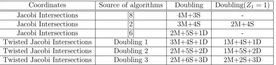
The comparison of the costs of above doubling formulae in this paper to those in previous works is listed in Table 1.
Doubling formulae independent of a and b. From aU2
1 = Z12 − V12
and bU2
Table 1: Algorithm comparison with other algorithms in Doubling
Coordinates Source of algorithms Doubling Doubling(Z1 = 1)
Jacobi Intersections [8] 4M+3S
-Jacobi Intersections [2] 3M+4S 2M+4S
Jacobi Intersections [6] 2M+5S+1D
-Twisted Jacobi Intersections Doubling 1 3M+4S+1D 1M+4S+1D
Twisted Jacobi Intersections Doubling 2 2M+5S+2D 1M+5S+2D
Twisted Jacobi Intersections Doubling 3 2M+6S+3D 2M+2S+3D
independent of the parameters a and b:
U3 = 2U1V1W1Z1, V3 =V12Z12−Z12W12+V12W12,
W3 = W12Z12−V12Z12+V12W12, Z3 =V12Z12+Z12W12−V12W12.
Addition formulae independent of a and b
Theorem 6. LetP = (u1, v1, w1), Q= (u2, v2, w2)be two different points on
the twisted Jacobi intersections elliptic curve Ea,b: au2+v2 = 1, bu2+w2 =
1, and letR =P+Q= (u3, v3, w3). Then the addition formulae can be given
by
u3 =
u2 1−u22
u1v2w2−v1w1u2
, v3 =
u1v1w2−w1u2v2
u1v2w2−v1w1u2
, w3 =
u1w1v2−v1u2w2
u1v2w2−v1w1u2
.
Proof. From
(u21−u22)(v22+au22w21) = u21v22+au21w21u22−u22v22−au22u22w12
=u2
1v22+ (1−v12)w12u22−u22v22−(1−v22)u22w12
=u2
1v22−u22v22 +u22v22w12−v12w12u22
=u21v22−u22v22(1−w21)−v12w21u22
=u2
1v22−bu21u22v22−v21w21u22
=u2
1v22(1−bu22)−v21w21u22
=u21v22w22−v12w12u22
we have
u2 1 −u22
u1v2w2 −v1w1u2
= u1v2w2+v1w1u2
v2
2 +au22w21
.
From
(u1v1w2−w1u2v2)(u1v2w2+v1w1u2)
=u2
1v1v2w22+u1u2v12w1w2−u1u2v22w1w2−u22v1v2w12
=u21v1v2(1−bu22) +u1u2w1w2(1−au21)−u1u2(1−au22)w1w2−u22v1v2(1−bu21)
=u2
1v1v2 −au21u1u2w1w2−u22v1v2+au22u1u2w1w2
= (u2
1−u22)(v1v2−au1w1u2w2),
we have
v1v2−au1w1u2w2
v2
2 +au22w21
= (u1v1w2−w1u2v2)(u1v2w2+v1w1u2) (u2
1−u22)(v22+au22w21)
= u1v1w2−w1u2v2 (u2
1−u22)(v22+au22w21)
u1v2w2 +v1w1u2
= u1v1w2 −w1u2v2
u1v2w2 −v1w1u2
.
Again, from
(u1w1v2−v1u2w2)(u1v2w2+v1w1u2)
=u21w1w2v22+u1u2v1v2w12−u1u2v1v2w22−u22v12w1w2
=u2
1w1w2(1−au22) +u1u2v1v2(1−bu21)−u1u2v1v2(1−bu22)−u22w1w2(1−au21)
=u2
1w1w2−bu21u1v1u2v2−u22w1w2+bu22u1v1u2v2
= (u21−u22)(w1w2−bu1v1u2v2),
we have
w1w2−bu1v1u2v2
v2
2 +au22w21
= (u1w1v2−v1u2w2)(u1v2w2 +v1w1u2) (u2
1−u22)(v22+au22w21)
= u1w1v2−v1u2w2 (u2
1−u22)(v22+au22w21)
u1v2w2+v1w1u2
= u1w1v2−v1u2w2
u1v2w2−v1w1u2
.
The formulae fail for point doubling. In addition, there are exceptional cases. For example, when 2P = 2Q, then the formulae cannot work. The above formulae in projective homogenous coordinates are given by the following theorem.
Theorem 7. Let P = (U1 : V1 : W1 : Z1), Q = (U2 : V2 : W2 : Z2) be two
different points on the twisted Jacobi intersections elliptic curve Ea,b: aU2+
V2 =Z2, bU2+W2 =Z2, and let R =P +Q = (U3 : V3 :W3 :Z3). Then
the addition formulae can be given by
U3 = U12Z22−Z12U22, V3 =U1V1W2Z2−W1Z1U2V2,
W3 = U1W1V2Z2−V1Z1U2W2, Z3 =U1Z1V2W2−V1W1U2Z2.
The projective addition formulae in Theorems 5 and 7 have exceptional points in each case. But the following theorem tells us that the formulae together in Theorems 5 and 7 cover all points.
Theorem 8. Let P = (U1 : V1 : W1 : Z1), Q = (U2 : V2 : W2 : Z2) be two
points on the twisted Jacobi intersections elliptic curve Ea,b : aU2 +V2 =
Z2, bU2+W2 = Z2 defined over K with ab(a−b) 6= 0, let R = (U
3 : V3 :
W3 :Z3) and S = (U
0
3 :V
0
3 :W
0
3 :Z
0
3), where
U3 = U1Z1V2W2+V1W1U2Z2, V3 =V1Z1V2Z2−aU1W1U2W2,
W3 = W1Z1W2Z2−bU1V1U2V2, Z3 =Z12V22+aU22W12,
and
U30 = U12Z22 −Z12U22, V30 =U1V1W2Z2−W1Z1U2V2,
W30 = U1W1V2Z2−V1Z1U2W2, Z
0
3 =U1Z1V2W2−V1W1U2Z2.
Then P +Q=R =S if R=S, and P +Q=R (orS) if S = 0 (or R= 0).
Proof. If R 6= (0,0,0,0), then R ∈ Ea,b and P +Q =R. Similarly, if S 6=
(0,0,0,0), then S ∈Ea,b and P +Q =S. Now assume R =S = (0,0,0,0).
Then U1Z1V2W2 +V1W1U2Z2 = 0 and U1Z1V2W2 −V1W1U2Z2 = 0. Thus
U1Z1V2W2 =V1W1U2Z2 = 0.
IfU1 = 0, thenZ12U22 = 0 sinceU12Z22−Z12U22 = 0. ThusZ1 = 0 orU2 = 0.
Therefore P = (0,0,0,0), which is contradict to P ∈ Ea,b. When U2 = 0,
then V1Z1V2Z2 = 0 from V3 = V1Z1V2Z2 −aU1W1U2W2 = 0. We can get
Q= (0,0,0,0) by the similar argument as above. Contradict to Q∈Ea,b.
The similar argument works for the cases when U2 = 0, Z1 = 0, Z2 = 0,
V2 = 0, W2 = 0, V1 = 0 or W1 = 0.
IfP 6=Q, From Theorem 7 we know thatP+Q=R=SifR6= (0,0,0,0) and S 6= (0,0,0,0).
Remark. The above Theorem give a complete addition laws for the curve
Ea,b : aU2+V2 =Z2, bU2+W2 =Z2 defined overK withab(a−b)6= 0. The
addition laws in the theorem cover all possible pairs of points on curvesEa,b.
New Addition algorithm use Theorem 7. The following formulae com-pute (U3 : V3 : W3 : Z3) = (U1 :V1 : W1 :Z1) + (U2 : V2 :W2 : Z2) in 15M,
We denote the algorithm by ”Independent.1”.
A = U1Z2; B =U2Z1; C =V1W2; D=V2W1;
E = U1Z1; F =V1W1; G=U2Z2; H =V2W2;
U3 = (A+B)(A−B);
V3 = AC−BD; W3 =AD−BC; Z3 =EH−F G.
Note that U3 = U12(bU22 +W22)−U22(bU12 +W12) = U12W22 −U22W12. If the
points represented by the sextuplet (U, V, W, Z, U W, V Z), then the addition formula can by modified by: (U3 :V3 : W3 :Z3 : M3 :N3) = (U1 : V1 : W1 :
Z1 : M1 : N1) + (U2 : V2 : W2 : Z2 : M2 : N2), where M1 = U1W1, N1 =
V1Z1, M2 = U2W2, N2 = V2Z2, the cost are 13M. We denote the algorithm
be ”MIndependent.2”.
A = U1W2; B =U2W1; C=V1Z2; D=V2Z1;
U3 = (A+B)(A−B);
V3 = AC−BD; W3 =M1N2−M2N1; Z3 =AD−BC;
M3 = U3W3, N3 =V3Z3.
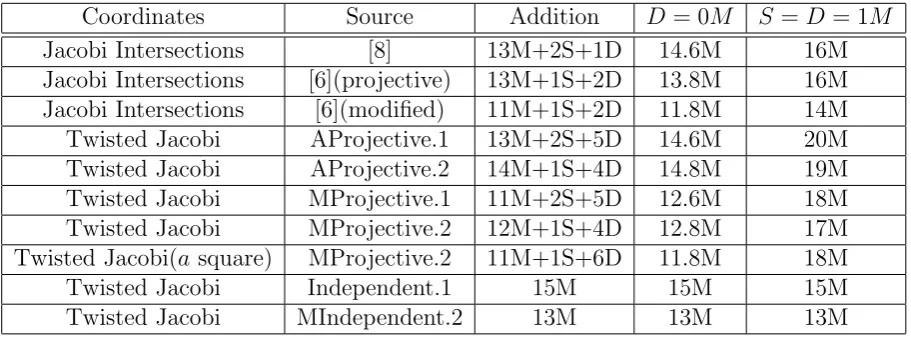
The comparison of the costs of above addition formulae in this paper to those in previous works is listed in Table 2.
Table 2: Algorithm comparison with other algorithms in addition
Coordinates Source Addition D= 0M S =D= 1M
Jacobi Intersections [8] 13M+2S+1D 14.6M 16M
Jacobi Intersections [6](projective) 13M+1S+2D 13.8M 16M
Jacobi Intersections [6](modified) 11M+1S+2D 11.8M 14M
Twisted Jacobi AProjective.1 13M+2S+5D 14.6M 20M
Twisted Jacobi AProjective.2 14M+1S+4D 14.8M 19M
Twisted Jacobi MProjective.1 11M+2S+5D 12.6M 18M
Twisted Jacobi MProjective.2 12M+1S+4D 12.8M 17M
Twisted Jacobi(a square) MProjective.2 11M+1S+6D 11.8M 18M
Twisted Jacobi Independent.1 15M 15M 15M
Twisted Jacobi MIndependent.2 13M 13M 13M
4
Jacobi versus Twisted Jacobi
The twisted Jacobi intersection curve is a generalization of Jacobi inter-sections, and twisted Jacobi intersection curve cover more elliptic curves than Jacobi intersections curves do. An example in [2] shows that for prime
p= 2255−19, one multiplication by 121665 and one multiplication by 121666,
which together are faster than a multiplication by 208003386839886583686474
08995589388737092878452977063003340006470870624536394≡121665/121666 (modp). That is, for a large parameter b of Jacobi intersections curves U2 +V2 =
Z2, bU2 +W2 =Z2, we can choose smaller a0 and b0 such that the twisted
Jacobi intersections a0U2+V2 = Z2, b0U2+W2 =Z2 is quadratic twisted to it, but can save computation costs. For example, in algorithms MProjec-tive.1, if a, bare smaller and a=ε2 is a square element in the field, then we
can omit the multiplications by the small constants. ThusZ3 =F2+a·E2 =
(F +εE)2−2εH, and the algorithm cost 11M + 1S, which is more efficient
5
Conclusion
In this paper, the twisted Jacobi intersections which contains Jacobi intersec-tions as a special case is introduced. We show that every elliptic curve over the prime field with three points of order 2 is isomorphic to a twisted Jacobi intersections curve. Some fast explicit formulae for twisted Jacobi intersec-tions curve in projective coordinates are presented. These explicit formulae for addition and doubling are almost as fast as the Jacobi intersections. In addition, the scalar multiplication can be more effective in twisted Jacobi intersections than in Jacobi intersections. Finally, new addition formulae which are independent of parameters of curves are proposed and it can be more effective than the previous results in literature when D > 0.6M. At last, we hope the faster point operation formulae on twist Jacobi intersection can be proposed.
References
[1] D. J. Bernstein, and T. Lange, Explicit-formulae database. URL: http://www.hyperelliptic.org/EFD.
[2] D. J. Bernstein, P. Birkner, M. Joye, T. Lange, and C. Peters, Twisted Edwards curves, In AFRICACRYPT 2008, LNCS 5023, 389-405, Springer, 2008.
[3] D. J. Bernstein and T. Lange, Analysis and optimization of elliptic-curve single-scalar multiplication, Cryptology ePrint Archive, Report 2007/455.
[4] O. Billet and M. Joye, The Jacobi model of an elliptic curve and side-channel analysis, AAECC 2003, LNCS 2643, 34-42, Spriger-Verlag, 2003.
[5] D. V. Chudnovsky, and G. V. Chudnovsky, Sequences of numbers gen-erated by addition in formal groups and new primality and factorization tests, Advances in Applied Mathematics 7(1986), 385-434.
[7] H. Hisil, K. Koon-Ho Wong, G. Carter and Ed Dawson, Faster group operations on elliptic curves, In Proc. Seventh Australasian Information Security Conference (AISC 2009), Wellington, New Zealand. CRPIT, 98. Brankovic, L. and Susilo, W., Eds. ACS. 7-19.
[8] P.-Y. Liardet, and N. P. Smart, Preventing SPA/DPA in ECC systems using the Jacobi form, CHES 2001, LNCS 2162, 391-401, Springer, 2001.
[9] Lawrence C. Washington, Elliptic Curves: Number Theory and Cryp-tography, CRC Press, 2003.
[10] Joseph H. Silverman, The Arithmetic of Elliptic Curves, Springer-Verlag, 1986.
Appendix. Proof of Theorem 1
Proof. Let V be a projective variety given by the equation
au2+v2 =z2
bu2+w2 =z2.
Let P = [u, v, w, z] be a point of V. Suppose that z 6= 0, then we can consider the equation
au2 +v2 = 1
bu2+w2 = 1.
LetQ= (u, v, w) be a point on the curve defined by this equation. If the point Q is singular, then the rank of the following matrix cannot be 2.
2au 2v 0
2bu 0 2w
so −4buv = 4vw = 4auw = 0, i.e. uv =vw =uw = 0. Suppose u = 0, then v2 = 1, w2 = 1, contrary to vw = 0, hence u 6= 0, so v =w = 0. But then u2 = a−1 =b−1 contradicts to the condition a 6= b. Therefore, there is
not any singular point on V with z 6= 0. Similarly we can show that there is not any singular point on V with z = 0 either. So Ea,b is a smooth curve.
Next we show that Ea,b is isomorphic to an elliptic curve of the form
Let (u0, v0, w0) = (0,1,1) be a point on Eab. First, we parameterize the
solutions to au2 +v2 = 1. similar to the Example 2.3 in [9], Let u =t, v = 1 +mt. Then we have
at2+ (1 +mt)2 = 1,
which yields 2mt+ (a+m2)t2 = 0. Discarding the solution t = 0, we obtain t=−2m/(a+m2), hence
u=− 2m
a+m2, v =
a−m2
a+m2.
Since the tangent at this point has slopem= 0, that m = 0 corresponds to (u, v) = (0,1)(). Substituting into bu2+w2 = 1 yields
((a+m2)w)2 = (a+m2)2−4bm2 =m4+ (2a−4b)m2+a2.
Letr= (a+m2)w, then
r2 =m4+ 2(a−2b)m2+a2.
Let
x= 2a(r+a)
m2 , y =
4a2(r+a) + 4a(a−2b)m2
m3 .
By Theorem 2.17 in [9] with q =a, the formulae then change this curve to the Weierstrass equation
y2 =x3+ 2(a−2b)x2−4a2x−8a2(a−2b) = (x+ 2a)(x−2a)(x+ 2a−4b).
The inverse transformation is
m= 2a(x+ 2a−4b)
y , r=−a+
m2x
2a .
The point (m, r) = (0, a) corresponds to the point (x, y) = ∞ and (m, r) = (0,−a) corresponds to (x, y) = (4b −2a,0). To synthesize the forward two steps, we obtain the following transformation.
ϕ:
x = 2a(
au2+(v−1)2 u2 w+a) (v−1)2
u2
= 2(au(v)−2(1)w2+1) + 2aw
y = 4a
2(au2+(v−1)2
u2 w+a)+4a(a−2b)( v−1
u ) 2
(v−1)3 u3
The inverse transformation is ψ :
u = −
4a(x+2a−4b) y
a+4a2(x+2a−4b)2 y2
= −y2+44y(ax(+2x+2a−a−4b4)b)2
v = a−
4a2(x+2a−4b)2 y2
a+4a2(x+2a−4b)2 y2
= yy22−+44aa((xx+2+2aa−−44bb))22
w = −a+
4a2(x+2a−4b)2x 2ay2
a+4a2(x+2a−4b)2 y2
= −yy22+4+2ax((xx+2+2aa−−44b)b2)2.
The point (u, v, w) = (0,1,1) corresponds to the point (x, y) = ∞ and (u, v, w) = (0,1,−1) corresponds to (x, y) = (4b−2a,0). The points (u, v, w) = (0,−1,1)and (u, v, w) = (0,−1,−1) correspond to the points (x, y) = (2a,0) and (x, y) = (−2a,0) respectively.
Substituting (x−2a)(x+ 2a)(x+ 2a−4b) fory2 in the expression ofψ,
and replacing (x, y) by (4x−2a,8y) yield the simpler equation
E :y2 =x(x−a)(x−b).
and simpler transformations.
ϕ:
x = −a(vw−+1)1
y = vau−1(x−b). , ψ :
u = −x22−yab
v = x2−x22−axab+ab
w = x2−x22−bxab+ab.
Now the point (u, v, w) = (0,1,1) corresponds to the point (x, y) = ∞and (u, v, w) = (0,1,−1) corresponds to (x, y) = (b,0). The points (u, v, w) = (0,−1,1)and (u, v, w) = (0,−1,−1) correspond to the points (x, y) = (a,0) and (x, y) = (0,0) respectively.
Since the curveEa,bandE are both smooth, then the rational mapϕand
its inverse map ψ are both morphisms by Proposition 2.1 in [10]. Therefore