POLARIZATION DIMENSIONALITY OF MULTI-ANTENNA SYSTEMS
M. S. Elnaggar
CALIT2
University of California San Diego
9500 Gilman Drive, La Jolla, CA 92093-0436, USA
S. K. Chaudhuri and S. Safavi-Naeini
ECE Department University of Waterloo
200 University Ave W, Waterloo, ON, N2L 3G1, Canada
Abstract—Based on the deterministic Maxwellian framework, we investigate the ability of each of the dual fields (electric and magnetic) in carrying independent information in a multi-polarization MIMO system. We quantify the performance by using a well-defined power independent dimensionality (PID) metric. We present numerical results for 3 deterministic scenarios: a canonical free-space (near and far field exact solution), a canonical PEC corridor (using rigorous modal analysis) and a lossy-wall corridor (using image ray tracing). The deterministic results show that in a multi-path rich environment, the hexapole system (collocated polarized electric and magnetic point radiators) is almost guaranteed to provide more than 3 DOF. However, in the simulated scenarios, the maximum 6 DOF are never attained due to the inevitable coupling between the electric and magnetic fields. On the other hand, for a tripole system, the upper-limit of 3 DOF is achievable.
1. INTRODUCTION
In this paper, we deterministically investigate the degree of freedom (DOF) gain (i.e., creation of new parallel channels) which can be provided through a collocated multi-polarization MIMO system. “Multi-polarization” designates transmit/receive collocated configurations, namely, tripoles (3 mutually-orthogonal collocated
point sources forming 3 independent ports), hexapoles (2 collocated dual tripoles i.e., electric and magnetic as described in [1, 2]), or other combined dual polarization cases.
The problem addressed in this work is eventually a single-point sampling (through infinitesimal electric/magnetic dipoles) of a vector-field which happens to experience 2 types of collocated spatial orthogonality: vectorial and (scalar)functional [2]. The former is the essence of the polarization diversity whereas one form of the latter is the pattern diversity in thefar-field modeling.
Various deterministic simulations in this work show that the vectorial and functional orthogonality are not necessarily independent due to the inevitable coupling between the electric and magnetic field components. Consequently, the claim of hexapole six-fold dimensionality gain [1, 2] under statistical channel assumption is not practically guaranteed. Certainly, the results of the deterministic simulations performed in this work cannot be strictly generalized to
every environment or even to a class of environments as is the case with the stochastic case. Nevertheless, such deterministic simulations accurately account (in the Maxwellian sense [5, 6]) for the coupling between the electric and magnetic fields, a feature which is overlooked in the statistical approach. We thus claim that the novelty of this work is the application of accurate deterministic techniques to draw some conclusions regarding the dimensionality of multi-polarized MIMO systems in the given environments.
We attempt to provide a clear answer to the following controversial question raised in the literature [1–4]: can each of the electric and magnetic fields carry an independent piece of information between 2 radiating structures and thus double the one-field communication dimensions? The challenge in this question lies in the fact that the 2 fields are not simultaneously arbitrary since they are related by Maxwell’s equations. Through a universal model sustained by numerical results, we show that the answer depends on the 2 inter-twined orthogonality types, which are environment-specific.
(LT). We conclude by showing a histogram of the multi-polarization dimensionality results of the simulated scenarios.
2. UNIVERSAL MULTI-POLARIZATION MODELING
In order to isolate the multi-polarization effect, we deliberately exclude the space diversity by employing collocated infinitesimal (Hertzian) dipoles as a perfect multi-polarization “field-probe”, having a zero-length and detecting the vectorial nature of the electromagnetic fields. Nevertheless, we must admit that the polarization diversity is inseparable of the pattern diversity, which ultimately makes the multi-polarization zero-length MIMO system founded on the combined pattern/polarization diversity. In fact, this double-diversity is the base of the 2 aforementioned types of collocated spatial orthogonality (vectorial and functional).
Similarly to [2], we employ the polarization matrix H6 ∈ C6×6,
which models the 6×6 MIMO channel between the transmit/receive hexapoles. For morn = {1,2,3}, the element hmn represents an
electrical receive/transmit, where (1,2,3) denote indices for the 3 mutually orthogonal coordinates. Similarly, formorn={4,5,6},hmn represents a magnetic receive/transmit, where (4,5,6) denote indices for the same 3 mutually orthogonal coordinates, respectively. We assume narrow-band operation of the system. Moreover, the following source normalization assumptions are made:
1. The electric (IEl) and magnetic (IMl) dipole moments are normalized such that (IMl) = η0(IEl), where η0 = 120π is the
free-space impedance.
2. The received signal, either by an electric or magnetic infinitesimal dipole, is detected as a proportional voltage. Therefore, any receive magnetic field component is multiplied by η0 in the
following analysis.
From the duality between the electric and magnetic fields [7], the hexapole channel matrixH6 is expressed as
H6=
C −D
D C
, (1)
where, for n = {1,2,3}, the column vectors c·n and d·n of the 3×3 sub-matrices C and D represent the receive electric and magnetic fields response, respectively, to the nth polarized transmit electrical
curl equations must be satisfied
∇ ×E = −jωµ0H (2a)
∇ ×H = jωε0E. (2b)
Therefore, from the aforementioned source-normalization assumptions and (2a), the sub-matrices Cand Dare related by
D=η0
¯ ∇ ×C −jωµ0
= j k0
¯
∇ ×C, (3)
where ¯∇ ×C is a dyadic curl (operating on the column vectors ofC) andk0 is the free space wave number. Accordingly,H6 is expressed as
H6=
C −j
k0
¯ ∇ ×C
j k0
¯
∇ ×C C
. (4)
Equation (4) isuniversal at anysource-free point in any environment as long as we are operating the system in narrow-band and the environment electrical/magnetic properties are deterministic at any one time. At any point in space where there is an impressed source or medium inhomogeneity (e.g., at the boundaries), (4) is not true.
Now, we return back to the question regarding the usage of E and H as independent information carriers. From (4), given the fact that the elements ofH6 are not all independent, can we really achieve 6 DOF? The answer was positive in [1, 2] and negative in [3, 4]. The deterministic results of this work provide evidence that by employing a hexapole system, wecan have more than 3 DOFif the environment permits. However, in all these deterministic simulations, the maximum 6 DOF have not been attained.
Hence, the core of the answer is how to exploit the 2 orthogonality types in the deterministic environment as modeled by H6. The
matrix rank becomes deficient when there exists a linear algebraic
dependence between the matrix rows or columns. In (4), there is a linear dependence, however, it isdifferential rather than algebraic and has therefore no clear impact on the matrix rank. The environment properties, manifested through the boundary conditions, set the explicit algebraic dependence between Cand D in (1). We will see in the upcoming case studies that whenever this differential dependence approximates a linear algebraic one (single plane-wave or spherical ray), only then, the rank becomes deficient.
along the 3 mutually orthogonal coordinates. Hence, the vectorial orthogonality is also known as the polarization diversity. If the dual fields (E andH) were independent (uncoupled), a pair of infinitesimal dual tripoles (electric and magnetic) would be sufficient to allow up to 6 DOF through independent vectorial orthogonality. However, the dual fields are indeed coupled; otherwise, the electromagnetic propagation would not exist. Therefore, in order to employ the DOF of the dual field, it is mandatory to have another sort of diversity, which is accomplished through the so-called Field Expansion Diversity (FED). The FED is also known as the functional orthogonality or, in the far-field analysis, pattern diversity. The terms functional orthogonality and FED are used interchangeably hereafter.
The FED is best understood when the received field is expressed as an integration (or summation in discrete analysis) of some field expansion components such as:
• The spherical propagating multipath rays in the case of high-frequency approximation (ray tracing). We emphasize that in this case, each ray should be considered inseparably of the transmit/receive pattern-weighting [2].
• In general, the plane-wave expansion components of the received field [8].
• The modes in a PEC waveguide, which can straightforwardly be further decomposed into a summation of plane waves.
At a given angular direction, an expansion component is individually rank-deficient of rank 2 [4]. Nevertheless, the integration (summation) of all the expansion componentscan produce a resultant higher rank matrix of better DOF [1, 2]. Consequently, a rank-deficient expansion component is not automatically a bottle-neck for the DOF of the multi-polarization MIMO system as was argued in [4]. In case of ray modeling, such FED is traditionally known as the antenna far-field
pattern diversity [2] since the weighted-integration (summation) of the multipath rays is done through the antenna patterns over the visible angular domain.
Within each plane-wave or spherical ray component, there is a linear algebraic dependence between the transverse electric and magnetic field components meaning that only one field can carry independent information. By only considering the independent electric field in each plane wave component, we have the following double-impact when all the plane-wave components impinge on a hexapole receive fromdifferent directions:
the electric field), the plane-wave integration/summation creates a third vectorial electric DOF because the resultant electric field now has 3 components [1].
• Each field component (say Ez) of an impinging plane wave has the potential to interact with 3 receive elements (electric z -polarized and transverse magnetic x-and y-polarized elements). However, these 3 receive elements interpret differently the same field component according to the plane-wave direction of arrival. Ultimately, when all the plane waves are angularly weighted (integration/summation), such functional orthogonality gives room to more DOF [2].
Therefore, in the hexapole system, we are exploiting the vectorial nature of one field along with the angular sensitivity of the
dual-field detector (rather than the dual-field itself, which is not independent) to convey independent information. Accordingly, the aforementioned question becomes whether the same mechanism (plane-wave expansion) can provide 2 independent orthogonality effects. The numerical results obtained in this work show that there is an inevitable coupling between these 2 orthogonality effects.
3. A CANONICAL FREE-SPACE MULTI-POLARIZATION SCENARIO
In this section, we investigate the dependence of the multi-polarized MIMO system DOF on the transmit/receive separation in free-space (near and far field). We employ a recently developed power-independent dimensionality (PID) metric [11] for the purpose of DOF evaluation throughout this paper. The PID definition and relevant properties are briefly stated in Appendix A. The justification of such a power-independent perspective in MIMO dimensionality evaluation is also discussed in Appendix A.
For a z-polarized infinitesimal electrical dipole in free space, the
coordinates are given by [9]
Er = (IEl)η0
cosθ 2πr2
1 + 1 jk0r
e−jk0r
Eθ =j(IEl)η0
k0sinθ
4πr
1 + 1 jk0r −
1
(k0r)2
e−jk0r
Hϕ =j(IEl)
k0sinθ
4πr
1 + 1 jk0r
e−jk0r
Eϕ =Hr =Hθ= 0
. (5)
By duality, for az-polarized infinitesimal magnetic dipole in free space, the field components are given by [9]
Hr = (IMl)
η0
cosθ 2πr2
1 + 1 jk0r
e−jk0r
Hθ =j (IMl)
η0
k0sinθ
4πr
1 + 1 jk0r −
1
(k0r)2
e−jk0r
Eϕ =−j(IMl)
k0sinθ
4πr
1 + 1 jk0r
e−jk0r
Er =Eθ =Hϕ = 0
. (6)
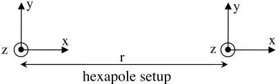
We begin by constructing the hexapole matrix and we follow the normalization assumptions of Section 2. We also assume an orientation as depicted in Fig. 1 for the transmit/receive hexapoles (2 broadside/1 endfire setup) and the hexapoles are separated by a distance r. Any arbitrary transmit/receive rotation is modeled by a unitary matrix with has no effect on the singular values of the channel matrix. This is true as well for other general scenarios.
x y z x y z r hexapole setup
Figure 1. Each end (transmit/receive) accommodates 2 collocated dual tripoles each consisting of 2 broadside and 1 endfire elements.
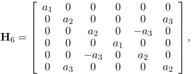
of the elements hmn denote the (x, y, z) coordinates for magnetic receive/transmit. According to Fig. 1, using (5) and (6) along with coordinate transformation and the aforementioned normalization assumptions,H6 is constructed yielding
H6=
a1 0 0 0 0 0
0 a2 0 0 0 a3
0 0 a2 0 −a3 0
0 0 0 a1 0 0
0 0 −a3 0 a2 0
0 a3 0 0 0 a2
, (7a)
where, after multiplying the field components by 4πr2 and omitting the common factors,
a1= 2
1 +ξ−1 a2=ξ+ 1 +ξ−1
a3=ξ+ 1
ξ =jk0r
. (7b)
Consequently, the singular values ofH6 are obtained from (7) yielding
σ{H6}={|a1|,|a1|,|a2+a3|,|a2+a3|,|a2−a3|,|a2−a3|}, (8)
where each singular value has a multiplicity of 2 [2].
In a similar fashion, we can extract from the generic H6 other
multi-polarization systems: • the 3×3 tripole matrixH3.
• the 4×4 tetrapole matrices H3e andH3b consisting of (1 tripole, 1 dual endfire) and (1 tripole, 1 dual broadside) polarizations, respectively.
• the 5×5 pentapole matricesH3ebandH3bbconsisting of (1 tripole, 1 dual endfire, 1 dual broadside) and (1 tripole, 2 dual broadside) polarizations, respectively.
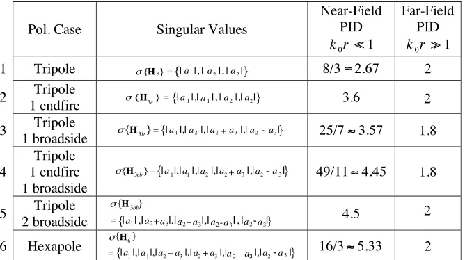
Table 1 includes the closed-form singular values as well as the near-field (a1/a2 → 2 and a3/a2 → 0) and far-field (a1/a2 → 0 and a3/a2 → 1)
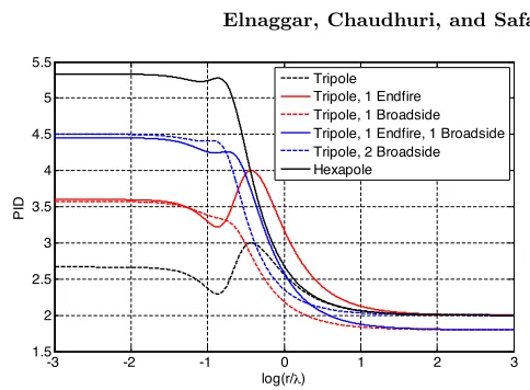
PID values. Fig. 2 depicts the distance-dependence of the PID for the multi-polarization scenarios.
The PID of case 1 and 2 in Table 1 reaches its maximum, rank (H), at one specific separation when |a1|=|a2|, which occurs at
r λ =
1 2π
5 +√37
Table 1. Summary of multi-polarization results.
Pol. Case Singular Values
Near-Field PID 0 1 k r Far-Field PID 0 1 k r
1 Tripole σ{H3 = |a|,| 2|,|a2| 8/3≈2.67 2
2 Tripole
1 endfire σ{H3e}={|a |,| 1|,|a2|,|a|} 3.6
3 Tripole
1 broadside σ{H3b}={|a |,| 2|,|a2 a3|,|a2-a3|} 25/7≈3.57 1.8
4
Tripole 1 endfire 1 broadside
{ }
3 1 2 2 3 2 3
{ eb} |a|,| |,|a |,|a a|,|a a |
σ H = - 49/11≈4.45 1.8
5 Tripole
2 broadside { } 3
1 2 3
{ }
| |,| |,| |,| |,| |
bb
a a a
σ
= +
H
4.5
6 Hexapole { }6
1 1 2 3 2 3 2 3 2 3
{ }
|a|,|a|,|a a |,| a|,|a a |,| a |
σ
= +
-H
16/3≈5.33 2
-<
< < <
2 2
2 }
} { 1 a
1 a
1
3
a a2+a3 a2-a3 a2
1 a +
+ a
a + -a
where λ is the free space wavelength. For all the other cases, the inevitable coupling between the electric and magnetic field prevents the PID from reaching rank (H) and the maximum PID occurs in the near-field region (k0r1).
In the far-field analysis, the spherical wave approaches a single traveling plane-wave (within a vicinity of some transmit/receive separation r to disregard the 1/r decay of the field). Therefore, the far-field scenario lacks any FED orthogonality since there is only one “plane-wave” component. Moreover, the absence of any field radial component reduces the vectorial orthogonality to 2. Consequently, we get the well-known horizontal and vertical polarization diversity for the hexapole system in the far-field region. From a matrix-modeling perspective, the far-field scenario approaches a matrix of rank 2, given the fact that there is a linear algebraic dependence between the transverse component of E and H. For case 3 and 4 in Table 1, the 2 channels have non-equal contributions{2|a2|,|a2|}. Therefore, from
a dimensionality perspective, case 3 and 4 dimensionality performance is less than 2.
-3 -2 -1 0 1 2 3 1.5
2 2.5 3 3.5 4 4.5 5 5.5
log(r/λ)
PI
D
Tripole Tripole, 1 Endfire Tripole, 1 Broadside Tripole, 1 Endfire, 1 Broadside Tripole, 2 Broadside Hexapole
Figure 2. PID vs r/λ (log-scale) for free-space multi-polarization scenarios.
multi-polarization. We use the plane-wave expansion of the spherical wave [8] to show that this near-field scenario, which seemingly has no multipath richness, is indeed super-rich. We assume a propagation hemisphere cross-section at z = 0 (the chosen decay direction of the evanescent components is along the positive z-axis). Comparing the field vector potential analysis to the plane-wave expansion of the field of an electrical point source, we get [8]
e−jk0r
r =
1 j2π
∞
−∞ ∞
−∞
e−jk0kˆ·r
kz
dkxdky, (10)
wherer= (x, y, z) is the position vector of the observation point with respect to the point source and ˆk = k1
0(kx, ky, kz) is a complex unit
vector (ˆk·ˆk = 1). According to our choice of the hemisphere cross-section at z = 0, kx and ky are always real (spanning the extended visible and evanescent angular domain). Accordingly, kz is either real or pure imaginary as follows:
• For kx2 +ky2 < k20, kz = +
k20−k2
x−ky2 (positive real) and ˆk is the propagation direction of the traveling plane wave component.
• For k2x + ky2 > k02, kz = −j
k2
x+k2y−k20 (negative pure
Because of the closed-form in the left-hand side of (10), we were able to exactly derive the field solution (5) and (6) in closed-form through Maxwell’s equations, and the solution includes all the evanescent waves components, which is not computationally available in the bounded electromagnetic problems. In the extended angular domain, the spectrum of (5) and (6) exhibits an ultra-wide spatial bandwidth
(traveling and evanescent). In other words, the near-field analysis of a free-space scenario resembles a super-rich multipath environment (including traveling and evanescent waves). Although each plane-wave (traveling or evanescent) has individually 2 DOF, the integration of all plane-wave components yields a higher DOF, which is against the argument of [4] concerning the strict upper limit of 2 DOF for the multi-polarization systems. Both the FED orthogonality and the existence of a radial field component (full vectorial orthogonality) contribute to this higher DOF. However, the coupling between the electric and magnetic fields does not allow the PID to reach the full-rank value of 6.
The multi-polarization near-field DOF results in this example gives an idea about theexpected DOF in a realistic multipath scenario: if a super-rich near-field environment does not achieve 6 DOF as already shown by rigorous analysis, it seems likely that most other environments may not achieve 6 DOF either. The results of the next section agree with this expectation.
4. MULTI-POLARIZATION IN A PEC CORRIDOR SCENARIO: MODAL ANALYSIS
We move now to investigate the multi-polarization DOF in a canonical indoor scenario. The environment is a rectangular open-ended corridor (waveguide) having PEC walls. Such a canonical structure is highly multipath-rich. We employ the modal field solution for this multi-polarization excitation under the PEC boundary conditions. The corridor width and height are 4 m and 3 m, respectively. The operating frequency is 2.4123 GHz, so chosen to avoid numerical complexity in the modal solution. Under these operating conditions (frequency and corridor dimensions), we have 2495 propagating modes.
L W H
Tx
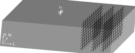
Figure 3. Multi-polarization scenarios in a corridor.
of all the evanescent modes.
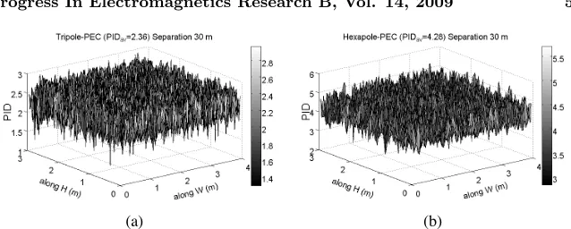
In the 3 simulated scenarios, we obtained very similar PID results. The average value for the PID for the tripoles and hexapoles systems over the grid locations is 2.35 and 4.3, respectively. An example of the PID over the grid points at 30 mL-separation is shown in Fig. 4. Very close average values were obtained as well when the transmit and grid points were re-located to other positions.
We can make several interesting observations from Fig. 4. In the hexapole case, 3 DOF or more are almost guaranteed. However, as expected earlier from the near-field free-space scenario, the full-rank 6 DOF have never been achieved in this rigorously-modeled multipath-rich environment. The reason for having less than full 6 DOF is attributed to the coupling between the electric and magnetic fields, which impacts the independence between the vectorial and functional orthogonality.
For the tripole scenario, the full-rank 3 DOF can be closely approached. Nevertheless, there are few occurrences of PID<2. In spite of the 2 DOF of each plane-wave component, their summation may accidentally yield lower dimensionality. This observation can be explained by a destructive interference that suppresses one out of the available 3 components of the electric field while there is a discrepancy in the values of the other 2 components (similar to case 3 and 4 in Table 1). In the hexapole case, such a suppression of 3 or more out of the 6 components of the electric and magnetic fields is very unlikely.
5. MULTI-POLARIZATION IN A TRANSPARENT-WALL CORRIDOR SCENARIO: IRT SIMULATION
(a) (b)
Figure 4. PID of multi-polarization MIMO system in a PEC corridor. The receive grid is located at 30 m from the transmit along L. (a) Tripole. (b) Hexapole.
thickness is 15 cm with a dielectric constant of 4 and a LT of 0.02. The ceiling and floor thicknesses are 30 cm with a dielectric constant of 6 and a LT of 0.05. We set up comparable scenarios to the PEC corridor in Section 4. The multi-polarized transmit is located at (50, 2, 2.8) along (L, W, H), respectively. The operating frequency is also 2.4123 GHz. The multi-polarized receive is moving over a grid of equidistant 20×20 points on the whole cross-section of the corridor. The simulation is repeated over 3 receive grids situated at 75, 80, 90 m along the L-axis as sketched in Fig. 3.
Such a transparent-wall corridor is a LOS environment and does not enjoy the same multipath richness as the PEC counterpart. We employ a 3D-IRT algorithm to evaluate the channel matrix at each receive grid point. The entries of H6 are constructed by applying the spherical ray expansion such that
hmn =
∞
l=1e (r)
ml
T ·D¯(rt)
l ·e
(t)
nl
exp (−jk0Rl) Rl
, (11)
where the index l represents the ray order; e(nlt) and e(mlr) are the transmit/receive farelectricfield pattern/polarization vector (effective length) at the proper ray departure/arrival direction, respectively, each
properties.
In order to readily obtain the far-field pattern/polarization (electric effective length) of a point electric current source, polarized in the ˆaξ direction, we use the following decomposition
e=−(ˆaξ·ˆaθ) ˆaθ−(ˆaξ·aˆϕ) ˆaϕ. (12) Then, to get the electric effective length of a point magnetic current
source, we apply the duality principle.
Since there is a linear algebraic dependence between the transverse components of the magnetic and electric field along each ray, the multipole PIDper ray can never exceed 2 (the vectorial orthogonality of one-field) and thus the IRT simulator needs to trace the electric field only. However, the summation (11) introduces a third vectorial DOF [1] as well as the functional orthogonality due to the pattern orthogonal weighting (pattern diversity or FED), which is modeled by
e(nlt) and e(mlr).
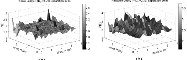
In [10], we found out that few hundred rays are sufficient to yield a convergent solution in the case of transparent walls (small LT). We employ in the simulations herein the most significant 1000 rays, which are traced from the fixed multi-polarization transmit to the moving multi-polarization receive at each grid point. Fig. 5 show the PID over the grid locations at a separation 30 m along L by using tripoles and hexapoles. The PID results are very similar in the other scenarios and the average PID is 1.9 and 2.4 for the tripole and hexapole systems, respectively. The lack of multipath-richness due to the transparent (lossy) walls has significantly reduced the DOF in comparison with the PEC corridor.
(a) (b)
6. DISCUSSION AND CONCLUSION
In this paper we investigated the DOF of a collocated multi-polarization antenna system in 3 case studies. The first 2 canonical cases, the near-field free-space and PEC corridor, represent rigorously derived multipath scenarios which are very rich. Unlike the stochastic-based simulations, the full-rank 6 DOF was never achieved through a hexapole system in the deterministic simulations herein.
Also, by applying the plane-wave (or spherical ray) expansion on the field in all the 3 studied cases, we showed that the individual 2 DOF per plane-wave component is not automatically a bottle-neck to the system DOF. The incoming plane waves at different directions result in a higher DOF of the system, which is attributed to the FED (also known as far-field pattern diversity or functional orthogonality) in addition to the obvious vectorial (polarization) orthogonality by creating one more component in the resultant field. However, it can happen that the total plane wave contribution yields less than 2 DOF as observed in the case of the tripole system in the PEC waveguide.
A rich multipath environment is needed in order to achieve an acceptable DOF performance through a multipole system. We repeated the PEC corridor simulations with the transmit multipole situated at various locations and we obtained very close average PID values for the tripole and hexapole systems as those of Fig. 4. One can argue that the open-ended PEC waveguide has only a hemi-spherical angular spread of the rays and thus it is not as multipath-rich as the optimum PEC enclosure. In order to examine this argument, we made other simulations in a PEC corridor with onlyone open end. We placed the transmit multipole and the receive grid atL = 50 and L= 75 m, respectively and a PEC wall is located at L = 100 m. Therefore, we have full angular spread over the receive spherical solid angle and the modal solution is still fast convergent (evanescent modes are suppressed). We repeated the modal analysis including the multipole source image and we obtained very similar results to Fig. 4, including the average PID values. Again, the maximum PID value of 6 has never been attained.
happen to be less than 2. On the other hand, the hexapole system almost guarantees more than 3 DOF, however, it never attains the full 6 DOF. The transparent-wall corridor, lacking multipath richness, yielded significant PID reduction and the gap between the tripole and hexapole PID average value decreases.
We conclude by summarizing the concepts and findings of this paperin the deterministic simulated scenarios:
• There are 2 types of collocated orthogonality (vectorial and functional) responsible for the diversity when using electric and magnetic multipole systems. These 2 types are inter-twined due to the inevitable coupling between the electric and magnetic field components.
• In a sufficiently multipath-rich environment, a tripole system may provide very close PID to the maximum full-rank 3 DOF. A hexapole system does not automatically double the tripole dimensionality (6 DOF were never achieved), however, the hexapole system produces, in general, higher DOF (more than 3 DOF are almost guaranteed).
• The average PID is environment-dependent (electrical proper-ties of boundaries) and seems to be independent of the deploy-ment configuration (location of the transmit/receive multipole el-ements). The gap between the hexapole and tripole PID values decreases as the multipath richness decreases.
ACKNOWLEDGMENT
This work was supported by the Natural Sciences and Engineering Research Council of Canada (NSERC) and in part by Research In Motion (RIM).
APPENDIX A. POWER INDEPENDENT DIMENSIONALITY METRIC (PID)
We treat the dimensionality as a power-independent indicator of the available parallel sub-channels of the system. Accordingly, we did not use the MIMO capacity, which is a global power-dependent metric, to evaluate the DOF. Rather, we developed a power independent dimensionality (PID) metric [11], which depends only on the singular values of the channel matrix.
A MIMO channel matrix H∈ CNR×NT, where (N
1 2 3 4 5 6 0
0.05 0.1 0.15 0.2 0.25 0.3 0.35 0.4 0.45
PID Histogram Tripole and Hexapole (Separation 30 m)
PID
Hist
ogram
Hexapole-PEC (PID
av=4.29)
Tripole-PEC (PIDav=2.36) Hexapole-lossy (PIDav=2.40) Tripole-lossy (PID
av=1.92)
(b)
1 2 3 4 5 6
0 0.05 0.1 0.15 0.2 0.25 0.3 0.35 0.4
PID Histogram Tripole and Hexapole (Separation 25 m)
PID
H
is
togram
Hexapole-PEC (PIDav=4.29) Tripole-PEC (PIDav=2.36) Hexapole-lossy (PIDav=2.31) Tripole-lossy (PID
av=1.87)
(a)
1 2 3 4 5 6
0 0.05 0.1 0.15 0.2 0.25 0.3 0.35
PID Histogram Tripole and Hexapole (Separation 40 m)
PID
Histo
g
ram
Hexapole-PEC (PIDav=4.31) Tripole-PEC (PIDav=2.36) Hexapole-lossy (PIDav=2.48) Tripole-lossy (PIDav=1.88)
(c)
channel H(eq), which has k equally contributing (out of K available) eigen channels whereas the remaining (K−k) sub-channels have zero contribution. Obviously, H(eq) hask communication dimensions and its singular values are given by
σ(ieq)=
σ0 i= 1,2, . . . , k
0 i=k+ 1, . . . , K . (A1)
Our target is to estimate an effective value forkaccording to some equivalence criteria betweenHandH(eq). Having 2 unknowns in (A1), σ0 and k, we need 2 equivalence conditions. We choose to impose p
-and q-Schatten-norm equivalence such that Hr ≡ H(eq)r, where r={p, q}. Accordingly,
k= PID∆ pq=
K
i=1
σqi
p K
i=1
σpi
qp−1q
p=q ∈ [1,∞). (A2)
The values for p and q are arbitrary. For large values of p and q, the Schatten norm tends to the spectral norm (the largest singular value). Therefore, a choice of small p and q makes the PID more sensitive to the small singular values. In this work, we chose the values p = 1 and q = 2. Thus, the PID used throughout the paper is given by
PID12=
K
i=1
σi
2 K
i=1
σ2i. (A3)
It can be shown that 1≤PIDpq(H)≤rank(H). Therefore, PIDpq(H) can be viewed as a well-defined effective rank of the matrixH.
REFERENCES
1. Andrews, M. R., P. Mitra, and R. De Carvalho, “Tripling the capacity of wireless communications using electromagnetic polarization,”Nature, Vol. 409, 316–318, Jan. 2001.
2. Svantesson, T., M. A. Jensen, and J. W. Wallace, “Analysis of electromagnetic field polarizations in multiantenna systems,”
IEEE Trans.Wireless Comm., Vol. 3, 641–646, Mar. 2004. 3. Piestun, R. and D. A. B. Miller, “Electromagnetic degrees of
4. Poon, A. S. Y., R. W. Brodersen, and D. N. C. Tse, “Degrees of freedom in multiple-antenna channels: A signal space approach,”
IEEE Trans.Information Theory, Vol. 51, 523–536, Feb. 2005. 5. Sarkar, T. K., M. Salazar-Palma, M. Wicks, and R. J. Bonneau,
Smart Antennas, John Wiley & Sons, 2003.
6. Sarkar, T. K., S. Burintramart, N. Yilmazer, S. Hwang, Y. Zhang, A. De, and M. Salazar-Palma, “A discussion about some of the principles/practices of wireless communication under a Maxwellian framework,” IEEE Trans.Antennas Propagation, Vol. 54, 3727–3745, Dec. 2006.
7. Harrington, R. F., Time-harmonic Electromagnetic Fields, McGraw-Hill, 1961.
8. Clemmow, P. C., The Plane Wave Spectrum Representation of Electromagnetic Fields, Oxford Pergamon Press, 1966.
9. Balanis, C., Antenna Theory Analysis and Design, John Wiley & Sons, 1997.
10. Elnaggar, M., S. Safavi-Naeini, and S. K. Chaudhuri, “Effect of oversimplifying the simulated indoor propagation on the deterministic MIMO capacity,” IEEE Canadian Conference on Electrical and Computer Engineering (CCECE 2004), Vol. 1, 219– 222, Niagara Falls, ON, May 2004.