Exact Box-Cox Analysis

(1)

Western University Western University

Scholarship@Western

Electronic Thesis and Dissertation Repository

4-13-2018 2:00 PM

Exact Box-Cox Analysis

Samira Soleymani

The University of Western Ontario

Supervisor

Dr. A. Ian McLeod

The University of Western Ontario

Graduate Program in Statistics and Actuarial Sciences

A thesis submitted in partial fulfillment of the requirements for the degree in Doctor of Philosophy

Follow this and additional works at: https://ir.lib.uwo.ca/etd

Recommended Citation Recommended Citation

Soleymani, Samira, "Exact Box-Cox Analysis" (2018). Electronic Thesis and Dissertation Repository. 5308.

https://ir.lib.uwo.ca/etd/5308

This Dissertation/Thesis is brought to you for free and open access by Scholarship@Western. It has been accepted for inclusion in Electronic Thesis and Dissertation Repository by an authorized administrator of

(2)

The Box-Cox method has been widely used to improve estimation accuracy in different fields, especially in econometrics and time series. In this thesis, we initially review the Box-Cox transformation [Box and Box-Cox, 1964] and other alternative parametric power transforma-tions. Following, the maximum likelihood method for the Box-Cox transformation is presented by discussing the problems of previous approaches in the literature.

This work consists of the exact analysis of Box-Cox transformation taking into account the truncation effect in the transformed domain. We introduce a new family of distributions for the Box-Cox transformation in the original and transformed data scales. A likelihood analysis of the Box-Cox distribution is presented when truncation is considered. It is shown that numerical problems may arise in prediction and simulation when the truncation effect is ignored.

A new algorithm has been developed for simulating Box-Cox transformed time series since previous methods are inefficient or unreliable. An application to sunspot data is discussed.

Box-Cox analysis is employed for random forest regression prediction using cross-validation instead of MLE to estimate the transformation. An application to Boston housing dataset demonstrates that this technique can substantially improve prediction accuracy.

Keywords: Box-Cox transformation, cross-validation, maximum likelihood, time series simulation, truncated distributions

(3)

Dedicated to my parents for their love, support and encouragement.

(4)

This thesis could not have been accomplished without the help of many people, to whom I am truly indebted for their valuable contributions. Through theses years of PhD, living in this warm family at Department of Statistical and Actuarial Sciences at Western University, I gained a big family where I can get energy to conquer all the future obstacles.

First and foremost I would like to express my sincere gratitude to my supervisor Dr. A. Ian McLeod for his invaluable guidance and generous support throughout my graduate experience at Western University. Without his encourage I would never accomplish the completion of my Ph.D journey. I am also grateful to all faculty, staff and fellow students at the Department of Statistical and Actuarial Sciences for their encouragement. Special thanks are also devoted to my examiners, Dr. Serge Provost, Dr. Sudhir Paul, Dr. Neil Klar and Dr. Jiandong Ren for their insightful comments and suggestions.

I am also indebted to my instructors at Western University, including but not limited to Dr. Wenqing He, Dr. Reg Kulperger, Dr. Hao Yu. I have the opportunity to work with, Dr. Duncan Murdoch, Dr. Hristo Sendov and Dr. Xiaoming Liu as their teaching assistant, and also Dr. David Bellhouse and Dr. Bethany White as their statistical consultant. Their encouragement and assistance are highly appreciated and will always be remembered.

Last but foremost, I would like to thank my father, Behzad, and mother, Nasrin for their perpetual and unconditional love and support through my life. I also would like to say thanks to my husband, Masoud and sister, Simin.

(5)

List of Figures

1.1 Time series plot of sunspots numbers. . . 13

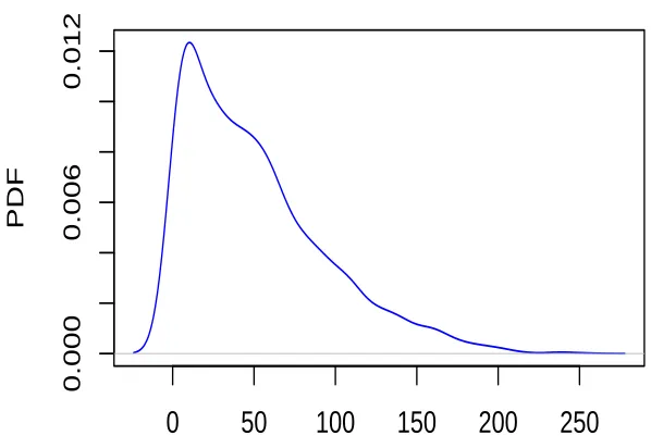
1.2 The probability density function using Gaussian kernel of sunspots. . . 13

1.3 Yeo-Johnson transformations was used. . . 14

1.4 Box-Cox transformations was used. . . 14

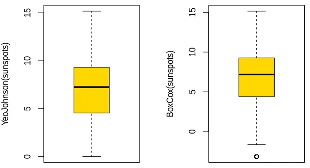
1.5 Comparison of the Yeo-Johnson transformed and Box-Cox transformed of sunspots data set. . . 15

1.6 Normal probability plot of the standardized prediction residuals of the fitted AR(9) model to original time series and Yeo-Johnson transformed time series withλ=0.318. . . 16

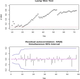
1.7 Diagnostic plots produced for AR(9) model fit to the Yeo-Johnson transforma-tion of yearly sunspot series. . . 16

1.8 Diagnostic plots produced for AR(9) model fit to the Box-Cox transformation of yearly sunspot series. . . 17

2.1 Weibull Distribution and a Box-Cox normal approximation. . . 28

2.2 Box-Cox Distributions with parametersλ = 1, µ = 0 and σ = 1. The exact Box-Cox normal distribution is a truncated normal distribution and its normal approximation distribution. The corresponding Box-Cox data distribution de-fined by the inverse Box-Cox transformation always has support on (0,∞). . . . 29

2.3 Plot of 1−κ, the probability that the inverse Box-Cox transformation is invalid when the Box-Cox approximation is used, vs. ξ, the standardized truncation limit. . . 30

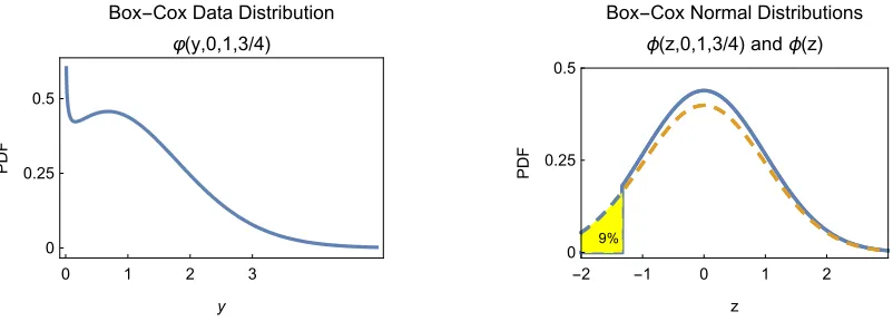
2.4 Box-Cox Data and Normal Distributions. In the right panel, the dashed curve shows the full normal distribution that is assumed in Box-Cox analysis. The yellow region corresponds to where the back-transform is invalid. . . 33

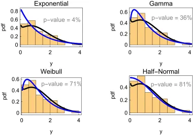
2.5 Data generated by the distributionϕ(y,0,1,3/4) is shown in the left panel and the histogram of the transformed data in the right panel. . . 34

2.6 Fitting some common Distributions to Box-Cox Data in the left panel of Figure 2.5. . . 35

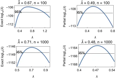
2.7 Exact and approximate likelihood analysis of simulated data from a Box-Cox data distribution with parameters µ = 0, σ = 1, λ = 0.75 for sample sizes n=100 andn=1000. . . 41

2.8 Histogram of ‘rivers’ dataset. . . 41

2.9 Exact and approximate likelihood analysis of ‘rivers’ dataset. . . 42

(8)

n=100 andn=1000. . . 43

2.11 Exact Box-Cox analysis with simulated regression with λ = 0.75 and µi = β0+βixi,i=1, . . . ,n . . . 45

2.12 Approximate Box-Cox analysis using R with simulated regression with λ = 0.75 andµi =β0+βixi,i= 1, . . . ,n . . . 45

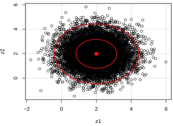
3.1 Ellipsoids of concentration corresponding to 0.95 and 0.5 probability for sim-ulated random variables from Box-Cox distribution with λ = 0.5, µ = 2 and σ=1. . . 50

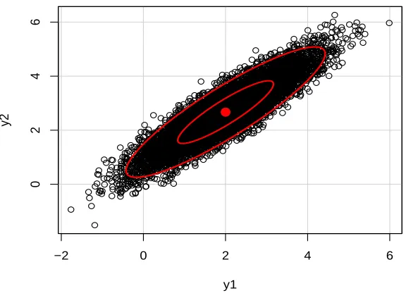
3.2 Ellipsoids of concentration corresponding to 0.95 and 0.5 probability for sim-ulated random variables from Box-Cox distribution withλ = 0.5 and ρ = 0.9 µ= 2 andσ =1. . . 51

3.3 Comparison between the simulated BoxCoxAR(1) time series with different Box-Cox transformationsλ= 0.25,0.5,0.75,1. . . 55

3.4 Comparison between the simulated BoxCoxAR(1) time series with different Box-Cox transformationsλ= −0.25,−0.5,−0.75,−1. . . 56

3.5 Simulated sunspot time series. . . 57

3.6 Yearly sunspot time series . . . 57

3.7 Theoretical and sample autocorrelations for simulated Box-Cox transformed time series. . . 57

3.8 Theoretical and sample autocorrelations for simulated back-transformed time series. . . 58

3.9 Time series plot of Ninemile time series . . . 60

3.10 Box-Cox analysis produced by BoxCox(Ninemile) for fitted AR(1). . . 61

3.11 Graph from boxcox for fitting ARp(1, 2, 6, 9) to Ninemile series. . . 61

3.12 Box-Cox transformed of Ninemile in transformed scale illustrated in first panel, and also simulation of transformed Ninemile series from fitted AR(1) model via bootstrap method as shown in the second panel. . . 62

3.13 Comparison of Box-Cox transformed Ninemile series and simulated Box-Cox transformed in the transformed data domain. . . 63

3.14 Simulate the BoxCoxARMA time series withλ=1. . . 66

3.15 Simulate the BoxCoxARMA time series withλ=0.5. . . 66

3.16 Simulate the transformed GuassianBoxCoxAR series withλ=0.5. . . 67

3.17 Simulate the GuassianBoxCoxAR time series withλ=0.5 in the original domain. 67 3.18 Simulate the transformed GuassianBoxCoxAR series withλ=1. . . 68

3.19 Simulate the GuassianBoxCoxAR time series withλ=1 in the original domain. 68 4.1 Median House Price, Training set shown. . . 70

4.2 Boxplot of the Training and Test residuals for random forest. . . 71

4.3 RMSE shown for random forest based on 100 replications. . . 71

(9)

List of Tables

1.1 Models fit to transformed yearly sunspot numbers time series. . . 17 1.2 Forecasts and their standard deviations for fitted AR(9) model to transformed

sunspot.year time series in terms of the Box-Cox and Yeo-Johnson transforma-tions. . . 18 3.1 Forecasts and their standard deviations at lead timel=1 for fitted AR(1) model

to simulated time series. . . 55 3.2 The theoretical probability of invalid back transform . . . 59 3.3 The true kappa based on 10,000 empirical simulations. . . 59 3.4 Theκand the probability of the Box-Cox normal approximation is failed shown

for Ninemile time series. . . 62 3.5 Different accuracy measures for simulated Box-Cox transformed AR(1) series

and Box-Cox transformed Ninemile. . . 63 4.1 RMSE comparison using average of 100 replications. . . 71 4.2 MAPE comparison using average of 100 replications for linear regression and

random forest. . . 72 4.3 MAPE various power transformation for random forest. . . 72 4.4 95% MOE for estimates shown in Table 4.3. . . 72

(10)

Introduction

In this chapter a review is presented regarding the parametric power transformations in regres-sion models and time series. Box and Cox [1964] proposed the Box-Cox transformation in order to improve the statistical models. It has been extensively studied on this subject with the most of the research concentrated on inferences about unknown parameters of interest [Box and Cox, 1964, Bickel and Doksum, 1981, Hinkley and Runger, 1984, Carroll and Ruppert, 1981].

In the literature, it was assumed that parametric family of distribution fromytoy(λ)withλ parameter are normally distributed with constant varianceσ2and meanµ. Therefore, the prob-ability density for inverse-transformed observations and likelihood function in original domain were obtained by multiplying the normal density distribution by the Jacobian of transforma-tion. The violation of the assumptions was sometimes ignored and statistical analysis was performed even though all assumptions were not satisfied.

In Chapter 2, we investigate the Box-Cox family distribution in the untransformed data domain by considering the truncation effect. Our next objective is to find that the optimal transformation would be changed by this assumption and how log-likelihood would be differed with respect to parameters λ, µ and σ. The exact Box-Cox distribution is shown and the comparison between an approximate and exact analysis is discussed in details. One of the controversial question would be regarding the estimation ofλ, and also it needs to explore that MLE would work under this assumption and limitation.

Chapter 2 explors the contribution of the exact Box-Cox analysis with application to rivers dataset. Initially, Chen and Lockhart [1997] obtained the conditional and unconditional infer-ences using parameter-based asymptotics for large finite sample size. Further, Chen et al. [2002] employed a large sample theory in the Box-Cox linear models and developed the goodness-of-fit test for the Box-Cox transformation. We illustrate the findings of Chapter 2 with simulated examples in a regression model, and compare them with some of the work done by previous researchers.

Finally, we revisit carefully the simulated truncated normal by Robert [1995], and we pro-pose an efficient algorithm for generating the Box-Cox transformed time series. It is presented an example of the truncation problem with Box-Cox analysis. Further, the modifications are performed for Durbin-Levinson algorithm to improve the simulation of the Box-Cox time se-ries.

This thesis reviews the transformation effect in linear regression, time series and Machine

(11)

1.1. Review of theBox-CoxTransformation 3

Learning. The simple power transformation is employed to minimize the expected prediction error.

1.1 Review of the Box-Cox Transformation

Transformation used to stabilize variance if variance changes with mean level of measurements [Bartlett, 1947]. Tukey [1957] introduced the power transformation to achieve normality of distribution or at least symmetrizing error distribution. This transformation is monotone and it preserves the order of data for λ > 0. Power transformations can be defined for positive random variable as,

Y(λ) =

      

Yλ, ifλ_,0,

log(Y), ifλ=0. (1.1)

Power transformations are often used in econometric and Kriging applications. The usual practice is to back transform data into the original data domain. Box and Tidwell [1962] con-centrated on the transformation of independent variables with no impact on homoscedasticity and normalization of error distribution. The Box-Cox transformation is a linear transformation of the power transformation but it is more suitable for mathematical treatment. For anyY > 0 andλR, the Box-Cox transformation is given by,

Y(λ) =

      

(Yλ−1)/λ, ifλ_,0,

log(Y), ifλ=0. (1.2)

Box and Cox [1964] suggested the Box-Cox transformation which can improve statistical mod-els by,

1. removing non-linearity; 2. removing heteroscedasticity;

3. removing skewness and non-normality of errors. The inverse Box-Cox transformation is obtained by,

Y =

      

(λY(λ)+₁₎1/λ, _ifλ

, 0,

exp(Y(λ)₎, _ifλ= ₀. (1.3)

Shifted power transformation was proposed to handle the negative observation [Box and Cox, 1964] as,

Y(λ) =

      

((Y+λ2)λ1 −1)/λ1, ifλ1 ,0,

log(Y+λ2), ifλ1 =0.

(12)

whereλ1 is the transformation parameter andλ2 is shifted parameter defined for Y +λ2 > 0.

This problem can be considered as non-regular case due to the restriction Y > −λ₂. The log-likelihood may not be determined by using the two parameter transformations since it approximately tends to infinity asλ2+min(Y)→ 0. Bickel and Doksum [1981] discussed the

signed power transformation such that,

Y(λ)= {sgn(Y)|Y|λ−1)}/λ, for λ >0. (1.5) which can cover the whole real number and there is no restriction on Y(λ)_{. This}

transforma-tion only can address the kurtosis rather than skewness of distributransforma-tion. The disadvantage of the signed power transformation is that it can not handle the skewed distribution. The initial assumption defined by Box and Cox [1964] restricted to positive data. Yeo and Johnson [2000] generalized the Box-Cox transformation in the case of the negative random variable.

The Yeo-Johnson transformation for a fixedλ,Y(λ):R→Ris defined by,

Y(λ)= Y(λ)(λ,Y)=

                  

(Y+1)λ−1/λ, ifY ≥ 0, λ_, 0, log(Y +1), ifY ≥ 0, λ= 0,

−(1−Y)2−λ−1/(2−λ), ifY < 0, λ_, 2,

−log(1−Y), ifY < 0, λ= 2.

(1.6)

where λ is power parameter likewise the Box-Cox transformation. This transformation can hold the properties of the log-mean standardization after the inverse-transformation sinceY(λ)

is invertible. Back-transformation is obtained by,

Y =                     

Y(λ)₍λ,_Y₎λ+₁1/λ₋₁, _if_Y(λ)₍λ,_Y₎,_≥ ₀, λ

,0, exp(Y(λ)(λ,Y))−1, ifY(λ)(λ,Y)≥0, λ= 0, 1−−Y(λ)(λ,Y)(2−λ)+11/(2−λ), ifY(λ)(λ,Y)<0, λ, 2, 1−exp−Y(λ)₍λ,_Y₎, _if_Y(λ)₍λ,_Y₎<₀, λ= ₂.

(1.7)

Lemma 1.1.1 From the Yeo-Johnson transformation, we can conclude the following results:

1. ForY ≥ 0, we haveY(λ)(λ,Y)≥ 0, and forY <0, it becomesY(λ)(λ,Y)<0; 2. Y(λ)(λ,Y) is continuous function in terms ofλandY;

3. Y(λ)(λ,Y) is convex withλ >1, and concave withλ <1.

1.2 Estimation of the Transformation Parameter

Box and Cox [1964] presented maximum likelihood and Bayesian approach for the estimation of the parameter λ. Maximum-likelihood estimates are obtained for a fixed λ by ignoring constant part as follows [Box and Cox, 1964],

logLmax(λ)=− n

2log( ˆσ

2

(13)

1.2. Estimation of theTransformationParameter 5

The robustness of the estimates of the parameters in a linear regression model have been ex-tensively studied and the truncation effect was neglected by Draper and Cox [1969], Atkinson [1973], Bickel and Doksum [1981], Carroll [1980], Hinkley and Runger [1984], Carroll and Ruppert [1981] and Taylor [1986]. Bickel and Doksum [1981] discussed the consistency of parameters via maximum likelihood estimation (MLE) and the asymptotic variance of these estimate in the regression. The ordinary likelihood function may be poorly behaved when the range of observations depends on unknown parameter or no local maximum found [Atkinson and Pericchi, 1991].

Bickel and Doksum [1981] assumed that Y(λ) = _h₍_Y, λ_{) can be defined as a monotone}

increasing transformation ofY in terms ofλin specific interval. Then,hhave partial derivation in terms ofY

J(Y, λ)=

n Y

i=1

hY(Yi, λ), (1.9)

where the Jacobian shown the mapping the (Y1, ...,Yn) → (h(Y1, λ), ...,h(Yn, λ)) and the mean

of the transformed variable can be written as,

µi(β)= p X

j=1

xi jβj, µ0i =µi(β0). (1.10)

The likelihood function is

L(Y, β, σ, λ)= 1 σn

n Y

i=1

f

      

Y_i(λ)−µi(β)

σ

     

J(λ,Y). (1.11)

The main differences between the model by Bickel and Doksum [1981] and Box and Cox [1964] is the use of arbitrary f instead of the normal distribution.

Inference discussion regarding the regression parameterβ andλwere presented in diff er-ent cases [Bickel and Doksum, 1981, Hinkley and Runger, 1984, Carroll and Ruppert, 1981]. Asymptotic calculations were presented such that the estimation of βis asymptotically more variable compare to standard linear model approach, therefore the changes of variance could be significant [Bickel and Doksum, 1981]. Carroll and Ruppert [1981] indicated that the inverse transformation used in order to make efficient inferences in original scale domain. Bickel and Doksum [1981] advocated that maximum likelihood estimates are sensitive to the distribution assumption. As a result, they concluded that it would be crucial to make the normal assumption of the response variable in linear model for inferences about regression coefficients.

The Box-Cox transformation assumes that the variable to be transformed is positive. Thus, in terms of definition, the Box-Cox transformation is intended to induce a truncated normal distribution. Poirier [1978] stated that it would be hard to determine whether the truncation effect is negligible since it depends on the unknown parameters of the distribution including the Box-Cox parameterλ. The Box-Cox transformation used in limited dependent variable (LDV) models with skewness for variables which have likely been censored or truncated [Poirier, 1978]. The estimation approach is to maximize the likelihood function of the truncated normal distribution.

(14)

nearly symmetrical distribution and it can be useful. Carroll [1980] suggested a new method to obtain robust estimator rather than likelihood method. Furthermore, approximate normality was investigated in theory and Monte-Carlo approach implemented in linear model.

Chen and Lockhart [1997] argued that the variances of parameter estimators increase based on ˆλand parameters are correlated. They derived the Fisher information matrix and its inverse for a general model involving regression as the truncation part was ignored. It was suggested that it can be considered the effect of truncation, but the analysis of likelihood function would be controversial. The models mentioned for the transformed and untransformed Box-Cox dis-tributions can be generalized by using exponential-family distribution as the error distribution. SupposeY_i(λ) are positive and independent variables with probability density functionφ(.) and cumulative distribution functionΦ(.) of standard normal. Moreover, we defineξ= −(λ−1+

µ)/σas a truncation point andY_i(λ)are the transformed variables. Let ˙Yi (λ)

and ¨Yi (λ)

be the first and second derivatives of Y_i(λ) with respect to λrespectively. The log-likelihood function in terms of the untransformed variable when truncation is negligible can be written,

logL(σ, µ, λ)= −n/2 logσ2− 1

2σ2 n X

i=1

y(_iλ)−µi

2

+(λ−1)

n X

i=1

logyi. (1.12)

In general, the Fisher information matrix for observation Yi by parameters θ = (σ, µ, β, λ)

obtained by,

1/n n X

i=1

σ2

Ii =                           

2 0 0 −2a

0 1 0 −b

0 0 Q −C

−2a −b −CT _d

                           (1.13) where

a=1/n n X

i=1

E        

(Y_i(λ)−µi) ˙Yi (λ) σ         , (1.14)

b= 1/n n X

i=1

EY˙i (λ)

, (1.15)

C =1/n n X

i=1

E[ ˙Yi (λ)

xi], (1.16)

d= 1/n n X

i=1

Eh(Y_i(λ)−µi) ¨Yi (λ)

+( ˙Yi (λ)

)2i, (1.17)

Q= 1/nXTX. (1.18)

(15)

1.2. Estimation of theTransformationParameter 7

variance of MLE ofθ. The inverse of the average information matrix is presented by,

Σ =      

1/n

n X

i=1

Ii        −1 =                                         1 2 + a2 f ab f

aCTQ−1 f

a f ab

f 1+

b2 f

bCT_Q−1

f

b f aQ−1_C

f

bQ−1_C

f Q

−1+ Q

−1_CCT_Q−1

f

Q−1_C

f a

f

b f

CTQ−1 f 1 f                                         (1.19)

whered−2a2−b2−CTQ−1C = f. It will be shown how to make inference about parameters whenλis unknown. Under regularity conditions, we can show that the distribution of ˆθcan be

approximated by, _√

n(ˆθ−θ)/σ ∼N(0,Σ). (1.20) Assumingλ= λ0is known, and let ˜β=βˆ(λ0) is independent of ˜σ=σˆ(λ0). Therefore, it would

be straightforward to make inference about parameters and it is given by

√

n( ˜β−β)/σ∼ N(0,Q−1), (n− p−1) ˜σ2∼ χ2_n₋_p₋₁, (1.21) and so we have

( ˜β−β)T_XT_X_{( ˜}β₋β₎

pσ˜2 ∼Fp,n−p−1, (1.22)

whereFp,n−p−1andχ2n−p−1are F-distribution andχ

2 _{distribution respectively.}

If we estimate λfrom data, the variance of ˆµand ˆσ can obtained from eqn. (1.19) and (1.20). It presented that the variance of both parameters, ˆµand ˆσ, can be increased as a result ofλestimation. There is the fact that usingFp,n−p−1for the unconditional inference onβis not

appropriate.

To construct a conditional inference in terms ofλ, it was discussed by Chen and Lockhart [1997] in details. Here, denote parameterθ = (σ, µ) and leth = √n( ˆλ−λ)/σ. Hence, we can compute the conditional distribution √n(ˆθ−θ)/σgivenh=h0in eqn. (1.20). It can be written,

√

n(ˆθ−θ)/σ|h=h0 ∼ N(m0,Σ0), (1.23)

and we have,

m0=          a

Q−1C

        

h0, (1.24)

and

Σ0 =         

1/2 0 0 Q−1

(16)

It seems that the covariance matrix for the conditional distribution is similar to the case λ known. In other words, F-distributionFp,n−p−1 can be used to make the conditional inferences

onβ.

Chen et al. [2002] considered limits as δ → 0, likewise Bickel and Doksum [1981] also used a limit whenδ → 0 asn → ∞. They assumed thatλandβare fixed, howeverδtends to zero asσ → 0. Probability density function in Box-Cox model can be affected by parameters as assuming fixedn. Chen et al. [2002] defined the two parameters such asθandφas follows

ˆ

θ=_β/ˆ _σ,_ˆ _φˆ ₌ _δ_{( ˆ}_λ−λ)/λ. (1.26) Consequently, it was concentrated on the asymptotic expansions of ˆφand ˆθby considering a limit and specific conditions. Draper and Cox [1969] and Taylor [1986] also mentioned to employ small parameterδfor the same expansion.

In Chapter 2, our work would provide the parameter ξ which is related to parameterδ = λσ/(1+λµ) indicated in Chen et al. [2002] and Bickel and Doksum [1981]. Bickel and Doksum provided a pretty poor approximation in asymptotic calculations ofβaround 0, this issue was criticized by several authors in application.

Yeo and Johnson [2000] assumed that transformed variables,Y(λ)(λ,Y1), ...,Y(λ)(λ,Yn) can

be considered as a normal distribution for someλ. Therefore, log-likelihood is given by,

logL(θ,Y)= −n/2 logσ2− 1

2σ2 n X

i=1

Y(λ)(λ,yi)−µ

2

+(λ−1)

n X

i=1

sgn(yi) log(|yi|+1), (1.27)

whereθ = (σ, µ, λ) andY(λ)(λ,yi) normally distributed withµandσ2. Maximizing L(θ,Y) in

terms of fixedλ, we have,

ˆ

µ(λ)= 1/n n X

i=1

Y(λ)(λ,yi), σˆ2(λ)= 1/n n X

i=1

Y(λ)(λ,yi)−µˆ(λ)

2

. (1.28)

Later, ˆλ is computed by maximizing profile log-likelihood function and so we obtain ˆθ = ( ˆσ2( ˆλ),µˆ( ˆλ),λˆ).

McLeod [2009] discussed the best symmetrizing transformation for four different distri-butions in Mathematica demonstration. The probability density function for the transformed random variable computed where λon [-2,2] and random variable with support on (0, ∞) in original domain. The specific value ofλwas shown for each of the distribution that removes the skewness of transformed random variable for all the distribution used [McLeod, 2009]. In general, the value ofλmay depend on the shape parameter in order to make symmetric distri-bution. McLeod [2009] stated that it would be possible to not find a symmetrizing transforma-tion for some distributransforma-tions including bimodal distributransforma-tion. Box-Cox power transformatransforma-tions are presented to use normal curve theory for non normal distribution of random variable [Griffith, 2013].

1.3 Transformations and Unbounded Likelihood Problem

(17)

1.3. Transformations andUnboundedLikelihoodProblem 9

[Box and Cox, 1964] to handle non-regular problems. It is assumed non-regular problem in the case that the distribution domain depends on the unknown shifted parameter. In theory, the maximum likelihood can not satisfy the regularity conditions if the range of the observations is defined by an unknown parameter. It is significant to denote the likelihood function as pro-portional of the probability functions. Montoya et al. [2009] criticized the strange behavior of profile likelihood functions which is derived by an unbounded density likelihood.

Cheng and Traylor [1995] expressed four types of non-regular problems in some situations and pointed out the unbounded likelihood as one of the special cases. Li et al. [2009] proposed EM algorithm for non-finite Fisher information if regularity conditions are failed to fulfill. In fact, unbounded behavior would lead to the problems in convergency and nonsense results for MLE. Liu et al. [2015] provided the “correct likelihood” to address the problem of unbounded likelihood by using small intervals.

Assuming a linear model for transformed valuesY(λ1, λ2) as follows,

Y(λ1, λ2)= Xβ+. (1.29)

Lety−_i(λ1, λ2) andy+i(λ1, λ2) define transformation asyi+ ∆andyi−∆used in eqn. (1.4). So,

the contribution ofyiin likelihood given by,

pi =

Φ(w+_i)−(w−_i ) 1−Φ(−xiβ/σ)

, (1.30)

wherew±_i =(Y±(λ1, λ2)−xiβ)/σandΦis standard normal distribution.

Grouped log-likelihood can be written as,

logL(λ1, λ2, β, σ)= n X

i=1

logpi−nlog(2∆). (1.31)

The correct likelihood was proposed by Liu et al. [2015] as a preliminary approach is given by,

L(θ)=

n Y

i=1

Li(θ;ti)= n Y

i=1

1 ∆i

[F(ti+ ∆i;θ)−F(ti−∆i;θ)], (1.32)

whereθis parameter and∆defined as the round-offerror. The round-offerror would present the estimated error in calculation by using rounding.

(18)

1.4 Non-Parametric Methods

Duan [1983] discussed the smearing estimate to predict the conditional mean of linear model after transformation. This model is non-parametric method used for expected response on the original domain. We have the estimation by the smearing estimate,

ˆ

E(Y0)= Z

h(x0βˆ+)dFˆn()=

1

n n X

t=1

h(x0βˆ+ˆ), (1.33)

and, if the distribution of errorF is not known, we estimate F function by empirical estimate as follows,

ˆ

Fn(e)=

1

n n X

t=1

I(ˆi ≤e), (1.34)

where ˆi = Y_i(λ)−xiβˆis the least squares residual andI(.) is defined as an indicator function.

We assume that g and h are monotone and continuous differentiable functions. Hence, it is defined by,

Y_i(λ)= g(Yi), Yi =h(Y_i(λ)).

Consistency and efficiency of estimate were investigated by Duan [1983] and then compared with a parametric method in regression model. Taylor [1986] also compared the conditional mean by smearing estimate and Taylor expansion in linear model. Gibbs Sampling can com-pute any desired expectation from posterior distribution. This approach is one of MCMC tech-nique. It was argued by Taylor [1986] that the bias of the small-θapproximation method could be reduced by using the higher order of expansion for the conditional mean, while the smearing estimator would tend to decrease variation of variance.

Breiman and Friedman [1985] provided non-parametric method to find optimal transfor-mation in multiple regression and stationary time series. The aim of this approach is the same as the Box-Cox transformation method. Alternating conditional expectation (ACE) algorithm was applied to different dataset for comparison. LetX1, ...,Xpbe mean zero stationary time

se-ries andθ,φ1, ...,φpare real valued function. Thus, the optimal transformations are computed

by minimizing the following function,

e2 = E

"

θ(Xp+1)− p P

i=1

φi(Xi)

#2

E[θ2₍_X p+1)]

. (1.35)

The procedure was initially implemented by Breiman and Friedman [1985] for simulated data when optimal transformations are given, and then it was applied to the Boston housing data of Harrison and Rubinfeld [1978].

(19)

1.5. Box-CoxTransformations andTimeSeries 11

is introduced by Foster et al. [2001] for the Box-Cox transformation without assuming normal distribution of the error term . It was illustrated by numerical simulation for the specific dataset, and also it was derived that estimators are consistent and asymptotically normal [Foster et al., 2001].

1.5 Box-Cox Transformations and Time Series

Maximum likelihood method applied to estimate the Box-Cox transformation parameterλand confidence interval forλin Box-Cox transformed family in AR model as follows,

z(tλ) =       

(zλt −1)/λ, ifλ, 0,

log(zt), ifλ= 0.

(1.36)

for time series datazt,t= 1, ...,n. Hipel and McLeod [1994] discussed this method for seasonal

and non-seasonal ARIMA model to obtain the z(tλ) series. Finally, the back-transformed time

series would be directly calculated from the ARMA or ARIMA model in the original data domain. Let log-likelihood function for an assumed valueλin AR(p) model be defined by,

logL(φ, λ)=−n

2log(S(φ)/n)− 1

2log(gn)+(1−λ)

n X

t=1

log(zt), (1.37)

and then maximizing over φ leads to L(λ) for λ. Using optimize function to maximize L(λ) function numerically which ˆλobtained. The relative likelihood function plot,R(λ)= L(λ)/L( ˆλ), illustrated a 95% confidence interval forλ. Box et al. [2008] discussed that the use of the Box-Cox transformation may improve the accuracy of the forecasts. Later, the Box-Box-Cox transfor-mation considered by Proietti and Riani [2009] for positive time series and multivariate time series. By using numerical and Monte Carlo integration, two conditional moments of season-ally adjusted time series were computed [Proietti and Riani, 2009]. Proietti and Riani [2009] developed a Taylor series expansion to determine the inverse transformation.

The optimal forecast for the seasonally adjusted series can be written as,

ˆ

zt = E(zt|Ft)=

Z +∞

−∞

(λz(tλ)+1) 1/λ

f(z(tλ)|Ft)dz(tλ), (1.38)

and, the conditional variance of the forecast error is presented by,

Var(zt|Ft)=

Z +∞

−∞

(zt−zˆt)2f(zt(λ)|Ft)dz(tλ). (1.39)

(20)

ˆ

zt =       

(1+λˆz(tλ))1/λ, ifλ, 0,

exp(ˆz(tλ)), ifλ= 0.

(1.40)

Granger and Newbold [1976] employed the Hermit polynomial expansion to compare the au-tocorrelation of data in the original data domain and transformed data domain. This method can be used by considering the Gaussian assumption of transformed time series. Consequently, they expressed that the original series is always less forecastable compare to the transformed series. Forecastability can be presented by [Granger and Newbold, 1976],

R2_h_,_z

t <R

2

h,z(_tλ), (1.41)

wherehis a lead time. Further, the autocorrelation of the transformed stationary Guassian time series can be defined ascorr(z(tλ),z

(λ)

t−k)= ρz(_tλ)(k). It was shown that,

|ρzt(k)|<|ρz(_tλ)(k)|. (1.42)

Furthermore, Granger and Newbold [1976] investigated loss function in the case of mean square error and mean absolute error. It needs to develop a numerical method for obtaining the optimal forecast for any specified loss function. The fact that the expected value of the inverse Box-Cox transformed can be considered as the minimum mean square error (MMSE) prediction, and the variance of the inverse transformed is its mean square error (MSE). Granger and Newbold [1976] discussed how their method can be extended to the homogenous non-stationary time series models which correspond to spatial models with the intrinsic non-stationary assumption.

1.6 Illustrative Application

It has been a problem to predict the sunspot numbers time series for several researchers and different forecasting methods have carried out in order to obtain the optimal forecast. In this section, the main goal is to explore the effect of two power transformations on the fitting model and forecasting.

(21)

1.6. IllustrativeApplication 13

sunspots

1750

1800

1850

1900

1950

0

50

150

250

Figure 1.1: Time series plot of sunspots numbers.

0

50

100

150

200

250

0.000

0.006

0.012

PDF

(22)

0.25 0.30 0.35 0.40

0.0

0.2

0.4

0.6

0.8

1.0

Relative Likelihood Analysis 95% Confidence Interval

λ

R(

λ

)

λ

^₌ 0.318

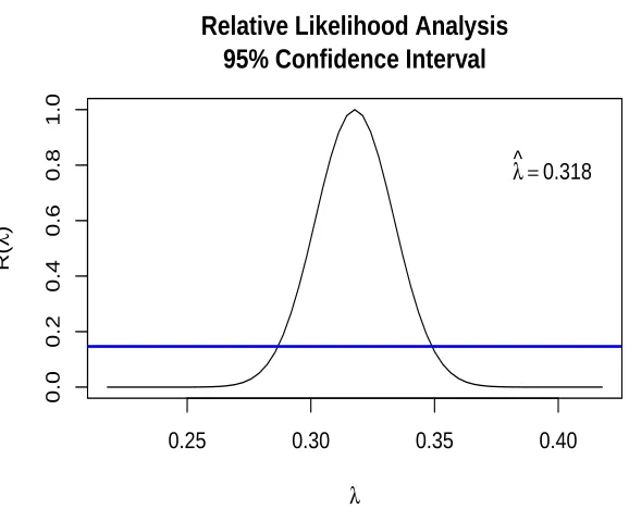
Figure 1.3: Yeo-Johnson transformations was used.

0.35 0.40 0.45 0.50

0.0

0.2

0.4

0.6

0.8

1.0

Relative Likelihood Analysis 95% Confidence Interval

λ

R(

λ

)

λ

^₌ 0.419

Figure 1.4: Box-Cox transformations was used.

(23)

variables can be derived. There is the fact that the Yeo-Johnson transformation can cover all range of (−∞,∞), hence it maybe provide more exact analysis compared to the Box-Cox transformation.

Therefore, we apply relative likelihood function to determine the optimal transformation, ˆ

λ. From Figure 1.3 and 1.4, we can conclude that ˆλbased on the Yeo-Johnson transformation is slightly smaller compared to the Box-Cox transformation for monthly sunspots time series. Furthermore, the Yoe-Johnson transformation produces slightly wider confidence interval for λwhenY > 0, and also ˆλ = 0.419 is not included in the confidence interval of the Box-Cox method. To produce Figure 1.3 and 1.4, additive shift used in both transformation. The 95% confidence interval forλcan be obtained by logL( ˆλ)−logL(λ)<1/2χ2

1,(1−α).

The boxplot shown below reveals that the Yeo-Johnson transformed data is more variable, but there is still some evidence of left skewness. The skewnesses are -0.14 and -0.20 for the Box-Cox and Yeo-Johnson transformed data respectively.

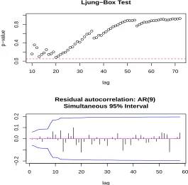
Figure 1.6 illustrates the normal probability of the residuals. The Box-Ljung portmanteau diagnostic plots produced for the Yeo-Johnson and Box-Cox transformed time series are shown in Figures 1.7 and 1.8. These diagnostic plots confirm that the AR(9) is a reasonable model for the both of the transformed data. From Figure 1.6, after transformation of the original time series, we can have an error distribution which behaves normal.

0

5

10

15

Y

eoJohnson(sunspots)

0

5

10

15

Bo

xCo

x(sunspots)

(24)

−3 −2 −1 0 1 2 3

−40

−20

0

20

40

60

Original Time Series

Theoretical Quantiles

Sample Quantiles

−3 −2 −1 0 1 2 3

−3

−2

−1

0

1

2

3

4

YeoJohnson Transformed Time Series

Theoretical Quantiles

Sample Quantiles

Figure 1.6: Normal probability plot of the standardized prediction residuals of the fitted AR(9) model to original time series and Yeo-Johnson transformed time series withλ=0.318.

10 20 30 40 50 60 70

0.0

0.2

0.4

0.6

0.8

1.0

Ljung−Box Test

lag

p−v

alue

0 10 20 30 40 50 60

−0.2

−0.1

0.0

0.1

0.2

lag

Residual autocorrelation: AR(9) Simultaneous 95% Interval

(25)

10 20 30 40 50 60 70

0.0

0.4

0.8

Ljung−Box Test

lag

p−v

alue

0 10 20 30 40 50 60

−0.2

0.0

0.1

0.2

lag

Residual autocorrelation: AR(9) Simultaneous 95% Interval

Figure 1.8: Diagnostic plots produced for AR(9) model fit to the Box-Cox transformation of yearly sunspot series.

BoxCox(sunspot.year) YeoJohnson(sunspot.year) Model AIC Portmanteau Diagnostic AIC Portmanteau Diagnostic

AR(2) 346.8 fail 120.6 fail

AR(9) 288.2 satisfactory 59.3 satisfactory

ARMA(2,1) 1168.62 borderline 942 borderline

Table 1.1: Models fit to transformed yearly sunspot numbers time series.

(26)

BoxCox(sunspot.year) YeoJohnson(sunspot.year)

Lead Forecast Standard deviation of forecast Forecast Standard deviation of forecast

1 17.271 1.583 12.419 1.065

2 17.877 2.483 12.728 1.662

3 17.129 2.925 12.283 1.948

Table 1.2: Forecasts and their standard deviations for fitted AR(9) model to transformed sunspot.year time series in terms of the Box-Cox and Yeo-Johnson transformations.

1.7 Maximum Likelihood Estimation

Fisher [1922] introduced the maximum-likelihood estimation technique following by Wald [1949] that discussed the asymptotic properties of MLE. The idea of modified likelihood method developed when the complete likelihood is difficult or impossible to calculate. Cox [1975] proposed the partial likelihood in the case it is more simpler than complete likelihood and also it only contains parameter interest rather than nuisance parameters. Conditional and marginal Likelihood methods are proposed to deal with some multiparameter problems. Sta-tistical inferences about the parameters of interest can be determined by eliminating nuisance parameters from likelihood function [Kalbfleisch and Sprott, 1970].

AssumeX1, ..., Xnbe a random variables from a population whose density depends on the

parameters θ and δ where are called a structural and incidental parameters respectively. To obtained the estimate of θ, conditional distribution was considered given minimal sufficient statistics forδ. DefineTi = T(xi) be the minimal sufficient statistic forδi and also probability

distributions of Ti be called g(ti|θ, δ). Thus, conditional distribution of X1, X2,..., Xn given T1= t1,...,Tn =tncan be written [Andersen, 1970] as,

φ(x1, ...,xn|θ,t1, ...,tn)= ∞ Y

i=1

φ(xi|θ,ti)= ∞ Y

i=1

f(Xi|θ, δi)/g(ti|θ, δ), (1.43)

whereTiis sufficient statistics forδdue to independency ofδ. The asymptotic normality of the

conditional maximum-likelihood estimation under assumptions defined as follows.

Theorem 1.7.1 The first and second derivatives oflog f(xi, θ,t)with respect toθexist for all

θin an open intervalΘ, and for allδis given by,

E ∂logφ(xi|θ,T)/∂θ= 0, (1.44)

andEh∂2logφ(xi|θ,T)/∂θ2 i

>0 and be continuous function ofδ.

(27)

1.8. EM Algorithm 19

Sprott [1970, 1973] described how conditional likelihoods may be useful in eliminating nui-sance parameters when the likelihood can be factored into two parts. There are two aspects to consider here would not be straightforward to express mathematically. First, variablesXshould include the all information required for the parameters of interest. Further, the distribution of

X is dependent on nuisance parameters. Secondly, nuisance parameters should not appear in the partial likelihood.

1.8 EM Algorithm

Statistical inference was mostly determined by MLE method as a result of its asymptotic nor-mality and efficiency properties. We propose EM algorithm which is more flexible and reliable to estimate parameters for truncated data. The EM algorithm is preferable over the numerical optimization because at each iteration the likelihood function increases and also the rate of convergency implies to stationary point. The EM process can be employed to determine the maximum likelihood estimate for censored and truncated data which come from exponential family [Dempster et al., 1977]. Lee and Scott [2012] illustrated the EM algorithm to fit mul-tivariate Gaussian mixture models on truncated and censored data. In general, if L(θ|y) has several stationary points, the convergency of EM sequence to local or global maximizers and saddle points depends on the choice of initial pointθ0 [Wu, 1983]. Cauchy distribution can be

considered as a non-regular case which its likelihood function with respect to location param-eter can be multimodal. Simulated annealing technique is performed to reach a global MLE with high probability for this special situations [Robert and Casella, 2004]. Furthermore, ge-netic optimization or Monte-Carlo Markov Chain (MCMC) would be applicable for this type of problem.

The EM procedure is very popular for computing maximum likelihood estimates from in-complete data, despite that fact that numerical optimization may be converged slowly. In the case where the likelihood function satisfies regularity conditions andL(θ|y) is unimodal unde-fined domain, the EM process convergences to unique MLE [McLachlan and Krishnan, 2007]. Dempster et al. [1977] suggested an algorithm to compute iteratively maximum likelihood es-timates for incomplete data including censored and truncated data. The EM approach contains two steps which each iteration of the expectation step (E-step) followed by the maximization step (M-step).

Suppose that observed data Yi, i = 1, ...,n have probability density function g(y|θ). Then we

can write,

g(y|θ)=

Z

f(y,z|θ)dz, (1.45)

and our main purpose is that the parameter can be obtained by,

ˆ

(28)

logL(θ|y)=log(g(y|θ)). (1.47) We assume that (Y,Z) as complete data have PDF f(y,z, θ) and log-likelihood of complete data can be written,

logLc(θ|z,y)= log(f(y,z|θ)). (1.48) The conditional density of incomplete dataZgiven observed dataY andθthen becomes,

k(z|y, θ)= f(y,z|θ)

g(y|θ) . (1.49)

So that, by taking logs

logg(y|θ)=log f(y,z|θ)−logk(z|y, θ). (1.50) We can define for givenθ0,

Eθ0logL(θ|y)=Eθ0[logL c

(θ|z,y)]−Eθ0[logk(z|y, θ)], (1.51)

where the expectation define in terms of distributionk(z|y, θ0). We only consider the first term

on the right side of eqn. (1.51) to achieve a maximizing logL(θ|y). By assuming the interchange expectation with respect toZand differentiation in terms ofθ0, let us have

∂θ0Eθ0[logk(z|y, θ)]= Eθ0∂θ0[logk(z|y, θ)]= 0. (1.52)

We consider the theory that the expectation of score function become zero [Casella and Berger, 2002]. We can conclude that∂θ0Eθ0[logk(z|y, θ)] is not depend on parameterθ, and then we can

maximizeEθ0[logL

c₍θ_|_z,_y_)].

We aim to maximize Q(θ|θ₀,y). Let us define,

Q(θ|θ₀,y)= Eθ0[logL c

(θ|z,y)]. (1.53) The iterative process begin with a given initial valueθ0 and letθj denote the value ofθafter j

cycles. The next cycle can be processed in two steps as follows,

1. E-step: compute the expected log-likelihood function of complete data,

Q(θ|θˆj,y)= Eθˆj[logL c

(θ|z,y)]. (1.54) 2. M-step: determine the parameterθj+1that maximize likelihood,

ˆ

θj+1 =argmax

θ Q(θ

(29)

1.8. EM Algorithm 21

1.8.1 General Properties of EM Algorithm

The EM process can be applied when data come from exponential family and then it is solv-able under the convexity property of log-likelihood including Jensenâ ˘A ´Zs inequality and the Kullback-Liebler discrepancy. We would present these concepts more in details and then use them in the derivation of the EM algorithm.

Theorem 1.8.1 Define f :X →R be a convex function if∀x1,x2 ∈X, and∀t∈[0,1]we have,

f tx1+(1−t)x2 ≤t f(x1)+(1−t)f(x2), (1.56)

so, it is called strictly convex if equality holds fort= 0 ort =1.

Theorem 1.8.2 Let p1, ..., pnbe Pr(Xi = x)= pi and f is a real continuous function which is convex. Then Jensen’s inequality given by,

f n X

i=1

pixi≤ n X

i=1

pif(xi). (1.57)

In general, we assume xas a random variable and f as any convex function whereE denoted expectation. Hence, it follows from Jensen’s inequality,

f E(x) _≤

E f(x).

(1.58)

Theorem 1.8.3 Jensen’s inequality is used to create the non-negativity of the Kullbach-Liebler discrepancy. Denote f(x) and g(x) be two probability density functions on R, the Kullbach-Liebler discrepancy is given by,

K(g, f)=

Z

log f(x)

g(x)f(x)dx= Ef log

f(x)

g(x). (1.59)

Proof

K(g, f)=

Z

log f(x)

g(x)

f(x)dx= − Z

log g(x)

f(x)

f(x)dx ≥ −log

Z

g(x)

f(x)

f(x)dx =0 (1.60)

We apply all theorem defined to show that likelihood increases at each step of EM algorithm. Using the sequences of ˆθj, j=0,1,2, ...given by the EM algorithm satisfy,

(30)

Equality yields in eqn. (1.61) if and only if,

Q(ˆθj+1|θˆj,y)= Q(ˆθj|θˆj,y), (1.62)

ProofBy using eqn. (1.51), it can be written as,

logL(θ|y)= Q(θ|θˆj,y)−Eθjlogk(z|y, θj). (1.63)

Hence we have,

logL(ˆθj+1|y)= Q(ˆθj+1|θˆj,y)−Eθjlogk(z|y, θj+1), (1.64)

and

logL(ˆθj|y)= Q(ˆθj|θˆj,y)−Eθjlogk(z|y, θj). (1.65)

Therefore, it was gained

(1.66) We present that by usingQ(ˆθj+1|θˆj,y)−Q(ˆθj|θˆj,y)≥0, eqn. (1.61) holds if we have,

Eθjlogk(z|y, θj+1)≤ Eθjlogk(z|y, θj). (1.67)

This can be written as,

Eθjlog

k(z|y, θj+1)

k(z|y, θj)

≥ 0. (1.68)

(31)

1.9. Appendix. InformationMatrix 23

1.9 Appendix. Information Matrix

Under regularity conditions, the MLE of ˆθis a consistent estimator ofθand also the asymptotic distribution of √n(ˆθ−θ) isN(0,Σ) whereΣcan be consistently estimated by ˆΣ =−h∂2L/∂θ∂θ´i

assessed at θ = θˆ [Cox and Hinkley, 1979]. Therefore, the information matrix is appropriate approach to estimate the approximate standard errors of the MLE estimates. For comparison with the truncated case, we first provide the result for random sampling from a complete normal distribution. It would be simpler to considerσrather thanσ2_{in finding the information matrix}

. In the normal IID case with complete data for a random sample of size n from a normal population with meanµand varianceσ2, the Fisher information matrix for (µ, σ) can be defined by,

I(µ, σ)=

             n

σ2 0

0 2n σ2              . (1.69)

In this part, we calculated expected information matrix in the more general case with consid-ering the truncation effect. Hence, denote

n X

i=1

Ii(σ, µ, β, λ)=                           

i11 i12 i13 i14

i21 i22 i23 i24

i31 i32 i33 i34

i41 i42 i43 i44                            . (1.70)

The log-likelihood,l(µ, σ, λ), can be written as follows,

logL(µ, σ, λ)=

n X

i=1

log       φ       

Y_i(λ)−µi

σ              +(λ −1) n X

i=1

log (Yi)−nlog(1−Φ(ξ)). (1.71)

Taking the first derivatives,

∂l

∂µ =

n X

i=1

(Y_i(λ)−µi)/σ2−n(1/σ)

φ(ξ)

1−Φ(ξ), (1.72)

whereΨ(ξ)=φ(ξ)/1−Φ(ξ) andξ= (T −µi)/σ.

(32)

∂2_l

∂µ2 =−

n

σ2 −(

n

σ)

∂φµ(ξ)(1−Φ(ξ))−(1−∂Φµ(ξ))φ(ξ) (1−Φ(ξ))2

!

=− n

σ2 −(

n

σ2)

ξφ(ξ)(1−Φ(ξ))−φ2(ξ) (1−Φ(ξ))2

!

=−nσ−2−nσ−2hξΨ(ξ)−Ψ2(ξ)i.

(1.73)

So, we have

i22 =−E

"∂₂

l

∂µ2 #

= nσ−21+ξE[Ψ(ξ)]−E[Ψ2(ξ)], (1.74)

and also, we can derivei13from eqn. (1.72)

∂2_l

∂µ∂λ = 1 σ2

n X

i=1

˙

Yi (λ)_.

(1.75)

Then, we obtain

i24 =−E

" ∂2_l

∂µ∂λ

#

=− 1

σ2 n X

i=1

E[ ˙Yi (λ)

]. (1.76)

To obtain the first derivative with respect toλ,

∂l ∂λ =− 1 σ2 n X

i=1

Y_i(λ)−µi ˙ Yi (λ) + n X

i=1

logYi. (1.77)

Next, differentiating with respect toλ

∂2_l

∂λ∂λ = 1 σ2

n X

i=1 h

¨

Yi (λ)

(Y_i(λ)−µi)+( ˙Yi (λ)

)2i. (1.78)

Hence, we derivei33

i44 =−E

" ∂2_l

∂λ∂λ

#

=− 1

σ2 n X

i=1

EhY¨i (λ)

(Y_i(λ)−µi)+Y˙i (λ)i

(33)

1.9. Appendix. InformationMatrix 25

Taking the second partial derivative with respect toσfrom eqn. (1.72),

∂2_l

∂µ∂σ ==−2σ

−3 n X

i=1

(Y_i(λ)−µi)+nσ −2h

Ψ(ξ)+ξ(ξΨ(ξ)+ Ψ2(ξ))i, (1.80)

so, we have

i21 =−E

" ∂2_l

∂µ∂σ

#

=−nσ−2hE[Ψ(ξ)]+ξ(ξE[Ψ(ξ)]+E[Ψ2(ξ)])i. (1.81)

To derivei11, we obtain the second partial derivative with respect toσ,

∂2_l

∂σ∂σ = nσ

−2₋₃_σ−4 n X

i=1

(Y_i(λ)−µi)2−nσ−2ξ h

−2Ψ(ξ)+ξ(ξΨ(ξ)−Ψ2(ξ))i. (1.82)

Thus, it given by

i11= −E

" ∂₂

l

∂σ∂σ

#

=2nσ−2+nσ−2ξh−2E[Ψ(ξ)]+ξ(ξE[Ψ(ξ)]−E[Ψ2(ξ)])i. (1.83)

From eqn. (1.77), we can obtain

∂2_l

∂λ∂σ =2σ

−3 n X

i=1

˙

Yi (λ)

(Y_i(λ)−µi). (1.84)

Then, we have

i14= −E

" ∂2_l

∂λ∂σ

#

=−2σ−2

n X

i=1

E[ ˙Yi (λ)

(Y_i(λ)−µi)/σ], (1.85)

and

i34 =−E

" ∂₂

l

∂λ∂β

#

= −σ−2 n X

i=1

E[ ˙Yi (λ)

xi], (1.86)

(34)

i33 =−E

" _∂₂

l

∂β∂β

#

= σ−2 n X

i=1

E[XXT]. (1.87)

The average Fisher information matrixI =σ2/n Pn

i=1Ii(σ, µ, β, λ)can be written by,

1

n n X

i=1

σ2_I i =                                      

2+ξw[−2+ξ2₋ξ_w_] ₋_w_[1+ξ2+ξ_w_] ₀ ₋₂_a

−w[1+ξ2+ξ_w_] ₁+_w₍ξ₋_w₎ ₀ ₋_b

0 0 Q −C

−2a −b −CT _d

                                      (1.88) where

w=E[Ψ(ξ)], (1.89)

a=1/n n X

i=1

E         ˙ Yi (λ)

(Y_i(λ)−µi)

σ         , (1.90)

b= 1/n n X

i=1

EhY˙i (λ)i

, (1.91)

C =1/n n X

i=1

EhY˙i (λ)

xi i

, (1.92)

d= 1/n n X

i=1

Eh(Y_i(λ)−µi) ¨Yi (λ)

+( ˙Yi (λ)

)2i, (1.93)

Q= 1/nXTX, (1.94)

whereΨ(.) = φ(.)/(1−Φ(.)) asλ > 0. In addition,Y_i(λ) assumed as the Box-Cox transformed variables where ˙Yi

(λ)

and ¨Yi (λ)

are the first and second derivatives ofY_i(λ). Therefore, the Fisher information for the exact Box-Cox likelihood can be defined using eqn. (1.88). By obtaining the Fisher information and its inverse, it can be noticed that the variance of the parameter estimators are dependent onΨ(ξ) whenλ >0. In other words, the first-order and second-order derivatives of log-likelihood in eqn. (1.71) associated with computing repeatedly these two fractions as follows. Forλ >0,

Ψ(ξ)= φ(ξ)/1−Φ(ξ), (1.95) and forλ <0,

(35)

Chapter 2 Exact Box-Cox Analysis

We will be working with various normal distributions so we introduce some convenient no-tations. Let φ(z, µ, σ) and Φ(z, µ, σ) denote the probability density function (PDF) and the cumulative density function (CDF) of a normal distribution with mean µ and standard devi-ation σ and let φ(z) = φ(z,0,1) and Φ(z) = Φ(z,0,1). The left and right truncated normal distribution functions with truncation point T are denoted respectively by φ(T,∞)(z, µ, σ) and

Φ(−∞,T)(z, µ, σ).

2.1 Introduction

Box and Cox [1964] introduced the idea for selecting a suitable power transformation by con-sidering the transformation as part of an enlarged model and showing how the transformation may be estimated by maximum likelihood (MLE). The Box-Cox transformation for random variableY is defined forY >0 by

Z = Y(λ) =

      

Yλ−1/λ, λ_,0,

log(Y), λ=0. (2.1)

With this definition the transformation is a continuous function of λ so the Jacobian of the transformationY → Zis a continuous and one-to-one.

Let Y be a positive random variable with probability density function (PDF) fY(y). Then

the PDF forZ =Y(λ)may be written,

fZ(z)=       

fY((1+zλ)1/λ)(1+zλ)1/λ−1, λ,0, λz+1> 0,

ezfY(ez), λ=0.

(2.2)

The transformation is used to improve the accuracy of the assumption of the normal distri-bution when the data exhibit skewness and other related non-normal features such outliers and monotone variance change. Often the transformation also improves the additivity assumption when used with the normal linear model. Figure 2.1 shows how the Weibull distribution can be made approximately normal with a suitable choice ofλ, viz. λ=0.416.

(36)

0 2 4 0

0.25 0.5

y

fY

(

y

)

Weilbull, shape=1.5, scale=1

-2 0 2

0 0.25 0.5

z

fZ

(

z

)

Transformed distribution,λ=0.416

Figure 2.1: Weibull Distribution and a Box-Cox normal approximation.

The inverse or back-transform,Z −→Y of the Box-Cox transformation may be written,

Y =

      

(λZ+1)1/λ, λ

,0,

exp(Z), λ=0. (2.3)

Box-Cox analysis [Box and Cox, 1964] proceeds by assuming the conditional distribution of the transformed variableY(λ)_{is normally distributed. eqn. (2.3) requires}λ_Y(λ)+₁> _{0 when}

λ _, 0. Hence we may conclude thatY(λ) has a truncated normal distribution. In the literature this truncation has been entirely ignored or assumed that it’s effect is negligible.

In this thesis we will demonstrate that this truncation may have an important effect.

2.1.1 The Box-Cox Distributions

In order to develop an exact treatment of Box-Cox analysis, we start by assuming the following data generation model (DGM). The DGM assumes there is a latent distribution in a sense similar to statistical models for censoring or missing values. In this case the latent distribution is a normal distribution that we refer to as theBox-Cox Normal Distribution. This distribution generates Z and then the observed data is generated by the inverse Box-Cox transformation, eqn. (2.3),Z → Y. The distribution ofY is referred to as theBox-Cox Data Distribution. It is a non-normal positive valued distribution which is implicitly defined by the distribution ofZ.

2.1.2 Box-Cox Normal Distribution

The PDF forZis proportional to the normal densityφ(Z, µ, σ) and the constant of proportion-ality is determined so the density integrates to 1 over the−λ−1_,_∞_{. Hence the density function}

forZ whenλ >0,

φ₍₋_λ−1_,_∞₎₍z, µ, σ)=

φ(z, µ, σ)

1−Φ(ξ). (2.4)

whereξ = −λ−1+µ.σ. Similarly, whenλ <0,

φ₍−∞,−λ−1₎₍z, µ, σ)=

φ(z, µ, σ)

(37)

2.1. Introduction 29

For the general case the Box-Cox Normal Distribution is,φ(z, µ, σ, λ), by

φ(z, µ, σ, λ)=

            

φ₍−λ−1_,_∞₎₍z, µ, σ), λ >0,

φ(z, µ, σ), λ= 0, φ₍−∞,−λ−1₎₍z, µ, σ), λ <0.

(2.6)

Standard Box-Cox analysis [Box and Cox, 1964] assumes the transformed data Z = Y(λ)

is normally distributed φ(z, µ, σ) and we will refer to this distribution as the Box-Cox nor-mal approximation. The right panel in Figure 2.2 compares the exact and Box-Cox nornor-mal approximation whenλ=1,µ=0 andσ= 1.

0 1 2 3

0 0.25 0.5

y

PDF

Box-Cox Data Distribution

φ(y,0,1,1)

16%

-2 -1 0 1 2 0

0.25 0.5

z

PDF

Box-Cox Normal Distributionϕ(z,0,1,1)

and Latent Normal Distributionϕ(z)

Figure 2.2: Box-Cox Distributions with parameters λ = 1, µ = 0 and σ = 1. The exact Box-Cox normal distribution is a truncated normal distribution and its normal approximation distribution. The corresponding Box-Cox data distribution defined by the inverse Box-Cox transformation always has support on (0,∞).

2.1.3 Kullback-Leibler Divergence

Box-Cox analysis [Box and Cox, 1964] ignores the effect of truncation and so assumes the distribution is normal,φ(z, µ, σ),−∞< z< ∞.The Kullback-Leibler (KL) divergence may be used to quantify the difference in terms of entropy between the approximate distribution and the exact true truncated distribution.

The KL divergence of the normal approximate distribution from the exact truncated normal distribution whenλ >0 is given by

K =

Z ∞

−λ−1

logφ(z, µ, σ)/(1−Φ(ξ)) φ(z, µ, σ)

! φ

(z, µ, σ) 1−Φ(ξ)dz

=−log(1−Φ(ξ))

1−Φ(ξ)

Z ∞

−λ−1

φ(z, µ, σ)dz

=−log(1−Φ(ξ)),

(38)

where

ξ=−λ −1+µ

σ . (2.8)

And similarly when λ < 0, K = −logΦ(ξ). When λ > 0, large−ξ corresponds to K 0 whereas forλ <0, large values ofξcorrespondK 0.

Letκbe the probability that the back-transform using the Box-Cox normal approximation is valid, that is,λZ+1>0. Then we have,

κ=

            

1−Φ(ξ), λ >0, 1, λ=0, Φ(ξ), λ <0.

(2.9)

Hence for the KL divergenceK, we haveκ=−eK_.

In Figure 2.2, 1− κ = Φ(−1) 16%. This means that if the Box-Cox normal approxi-mation was used to simulate data, it would fail about 16% of the time. In a simple situation involving only independent identical distributions, simply rejecting the invalid data would be an expedient solution but if 1−κwas close larger even this approach might not be feasible in more complicated models such as in regression and time series.

The exact Box-Cox Normal Distribution may also be written

φ(z, µ, σ, λ)=κ−1φ(z, µ, σ), z∈ R_λ, (2.10) whereRλ defines the feasible region forλin the transformed domain,

R_λ =             

z∈(−λ−1,∞), λ >0,

z∈(−∞,∞), λ= 0,

z∈(−∞,−λ−1), λ <0.

(2.11)

From Figure 2.3 we conclude that the accuracy improves as ξ −→ −∞ whenλ > 0 and when ξ −→ ∞when λ < 0. It is usually assumed that λ = 1 indicates no transformation is needed, but strictly speaking we need to also assume thatξ −3 so that the truncation effect can be neglected.

-3 0 3

0 1

ξ

1

-κ

λ>

0

-3 0 3

0 1

ξ

1

-κ

λ<

0

(39)

2.2. Simulation of theBox-CoxDataDistribution 31

2.1.4 Box-Cox Data Distribution

The distribution that generates the observationsy1, . . . ,ynis needed to construct the likelihood

function. The Box-Cox Normal Distribution,φ(z, µ, σ, λ), defines the distribution of the data in the transformed domain. Applying the inverse Box-Cox transformationZ →Y, the distribution of the data in the original domain is defined. This distribution is denoted by ϕ(y, µ, σ, λ) and is defined as the Box-Cox Data Distribution. Using eqn. (2.3) for the inverse transformation to substitute forzand using the Jacobian of the transformation, dyz= yλ−1, theexactBox-Cox

Data Distribution may be written,

ϕ(y, µ, σ, λ)=

            

φ₍−λ−1_,_∞₎ yλ−1

.

λ, µ, σ

yλ−1, λ >₀,

φ(log(y), µ, σ)y−1, λ=₀,

φ₍−∞,−λ−1₎ yλ−1

.

λ, µ, σ

yλ−1, λ <₀.

(2.12)

Since the Box-Cox distribution is only defined for Y > 0, the distribution ϕ(y, µ, σ, λ) has support on (0,∞) as required. To check this note that whenλ >0, (yλ−1)/λ ∈(−λ−1,_∞_{) if and}

only ify> 0. Similarly forλ <0. The special case,ϕ(y, µ, σ,0), is the log-normal distribution. Box and Cox [1964] implicitly assume for the likelihood computation the approximation that ϕ(y, µ, σ, λ) φ(y(λ))yλ−1. For data arising in applications, y > 0, so both the Box-Cox transformation and its inverse are valid. In computational statistical inference, such as the parametric bootstrap, this approximation may fail because the inverse Box-Cox transformation may be invalid when the Box-Cox approximate normal distribution is used.

2.2 Simulation of the Box-Cox Data Distribution

Simulation of data from the Box-Cox Data Distribution has important applications. In com-putational statistical inference, methods such as non-parametric bootstrapping, Monte-Carlo testing, Monte-Carlo Markov Chain and cross-validation where it is necessary to simulate data from a fitted hypothetical model. In civil engineering, synthetic or simulated data from empir-ical models are used for the engineering design. Since Box-Cox models are used in all these applications, it is essential to be able to reliably simulate data from fitted models.

The naive simulation method is simply to generate data from the complete normal distribu-tion and then use the inverse Box-Cox transformadistribu-tion to simulate the data in the untransformed domain. But as we have shown, there is a non-zero probability, 1−κthat inverse transformation may be undefined.

In general, the inverse CDF method may be used to generate data from theBox-Cox Normal Distribution. Then the Box-Cox transformation is employed to generate the random variates from the Box-Cox Data Distribution. This two-step method is usually necessary because the inverse CDF method can not usually be applied directly to theBox-Cox Data Distribution.

Whenλ > 0, the distribution ofZ, φ(−λ−1_,_∞₎(z, µ, σ) is a left-truncated normal with

param-etersµ, σ and truncation point,−λ−1. Our objective is to provide an algorithm to simulateZ

Exact Box-Cox Analysis

Scholarship@Western

Scholarship@Western

Exact Box-Cox Analysis

Exact Box-Cox Analysis

Dedicated to my parents for their love, support and encouragement.

Contents

List of Figures

List of Tables

Introduction

1.1

Review of the Box-Cox Transformation

1.2

Estimation of the Transformation Parameter

1.3

Transformations and Unbounded Likelihood Problem

1.4

Non-Parametric Methods

1.5

Box-Cox Transformations and Time Series

1.6

Illustrative Application

1750

1800

1850

1900

1950

0

50

100

150

200

250

1.7

Maximum Likelihood Estimation

1.8

EM Algorithm

1.8.1

General Properties of EM Algorithm

1.9

Appendix. Information Matrix

Chapter 2

Exact Box-Cox Analysis

2.1

Introduction

2.1.1

The Box-Cox Distributions

2.1.2

Box-Cox Normal Distribution

2.1.3

Kullback-Leibler Divergence

λ>

0

λ<

0

2.1.4

Box-Cox Data Distribution

2.2

Simulation of the Box-Cox Data Distribution