Small Linearization: Memory Friendly Solving of
Non-Linear Equations over Finite Fields
Christopher Wolf & Enrico Thomae Horst Görtz Institute for IT-security
Faculty of Mathematics
Ruhr-University of Bochum, 44780 Bochum, Germany {christopher.wolf,enrico.thomae}@ruhr-uni-bochum.de,
First Version: 2011-12-14
Abstract
Solving non-linear and in particular Multivariate Quadratic equations over nite elds is an important cryptanalytic problem. Apart from needing exponential time in general, we also need very large amounts of memory, namely≈N n2 fornvariables, solving degreeD, andN≈nD. Exploiting systematic structures in the linearization matrix, we show how we can reduce this amount of memory byn2to≈N. For practical problems, this is a signicant improvement and allows to t the overall
algorithm in the RAM of one machine, even for larger values ofn. Hence we call our technique Small Linearization (s`).
We achieve this by introducing a probabilistic version of the F5 criterion. It allows us to replace
(sparse) Gaussian Elimination by black box methods for solving the underlying linear algebra prob-lem. Therefore, we achive a drastic reduction in the algorithm's memory requirements. In addition, Small Linearization allows for far easier parallelization than algorithms using structured Gauss. Keywords: MultivariateQuadratic systems of equations, Finite Fields, F5, XL, HybridF5, Gröbner
Basis, XL, eXtended Linearization, Algebraic Cryptanalysis
1 Introduction
Solving systems of non-linear equations is a subject of intensive study for more than hundred years. In cryptanalysis, these systems proved particularly useful not only in the case of stream ciphers [Cou02, FM07], but also for block ciphers [MR02b, BPW06] and hash functions [SKPI07]. Similarly, it was possible using algebraic techniques to break asymmetric schemes such as variants of McEliece [FOPT10], MQ-schemes such as Hidden Field Equations [FJ03], or the Isomorphism of Polynomials identication scheme [Per05]. They are all subsumed under the term algebraic cryptanalysis.
A main drawback of algebraic cryptanalysis is the huge memory consumption, which is even the case for advanced methods such as HybridF5 [BFP09]. In this article we concentrate on the class of a
Gröbner Bases algorithms like F4, F5 and XL (eXtended Linearization) to solve equations of degree 2.
We call these equationsMultivariateQuadratic (MQ). Note that it is sucient to concentrate on them asMQis alreadyN P-complete [GJ79]. In addition, any systems of degree higher than 2 can be reduced eciently toMQ. In particular we show how to fuse F5 and XL into a variant that uses substantially
less memory than any other known solver of Multivariate Quadratic equations. Even for theoretical running times of above280, the amount of memory needed still ts into the RAM of a normal computer
(≈4 GB, cf. Sect. 4.4).
1.1 Related Work
For Gröbner basis algorithms, we compute the Gröbner basis of the ideal associated to the system P(x)by the mean of so-called S-Polynomials. This yields at least one univariate equation which we can
then solve. Main step forward in this area was the F4 algorithm [Fau99] as it computed S-Polynomials
blockwise rather than pairwise and thereby omitted many unnecessary steps in Buchberger's initial algorithm. It was later improved to the so-called F5 algorithm [Fau02b] which removed trivial syzygies
by keeping track of its computation through so-called signatures. For example, this algorithm was used to break HFE challenge 1 [Fau02a] in under 96 hours. To the knowledge of the authors, the fastest general purpose realization of F5 is the so-called hybrid strategy which was used to break many symmetric
and asymmetric challenges [BFP09]. However, there are also special instances of F5 for cryptographic
purposes [JV11]. We summarize the last three algorithms under the heading F-class.
In the case of XL algorithms, nding solutions for P(x) is reduced to linear algebra from the start
and a univariate equation over the ground eldFis obtained by producing a matrix in row echelon form.
As for the previous class, we can then solve the overall system, cf. Sect. 2 for more details. A rened version of this idea was given in [CKPS00]. In particular, linear dependencies were removed after each intermediate step. While there have been rumours that AES can be broken this way, they have later been discarded [MR02a]. However, this has seriously damaged the reputation of XL in the cryptographic community. Still, there was progress made in three areas. First, it was discovered that XL becomes more ecient by guessing r variables for some small value r ∈ N. This can be seen as a time-time
tradeo between O(qr)and the running time of XL for (n−r)variables. Second, Faugère and Joux
showed that a careful implementation of the linear algebra step can drastically reduce memory [FJ03, Sect. 5.2&5.3]. In fact, the idea sketched there is elaborated in Sect. 4.1. In addition, they provide a randomized version of the algorithm presented in Sect. 4 neglecting systematic linear dependencies between matrix rows. Third, XL was used in connection to sparse equation solvers such as Wiedemann. This way, the inherent problem of memory consumption was mitigated [YCBC07, ADK+10]. However,
the fact that the linear algebra to be solved was signicantly larger than for the F-class remained. Forth, the so-called Mutant strategy was invented to make use of values, which were previously discarded. As a result, XL was sped up by one order of magnitude [SAD+08] as the size of the matrix was signicantly
reduced. It is the most ecient representative of the XL class known to the authors.
During the last few years, both XL and F5 were treated as two rather dierent algorithms. In
addition, there was a heated discussion, which algorithm is better. In particular, Ars et al. [AFI+04]
showed that XL is a redundant version of F4, i.e. it produces more equations than necessary. As F5 is
always more ecient than F4, this was a devastating blow for the XL family. Moreover, in 2011 Albrecht
et al. [ACFP11] showed that even MutantXL is a redundant version of F4. A unifying attempt is due
to Albrecht who introduced the Matrix-F5 algorithm in [Alb10, Ch. 5]. This is an F5 version of the XL
algorithm. However, it is not competitive with F5in terms of speed or memory. In particular, the whole
matrix needs to be stored to compute the Gröbner basis. All in all, these results suggest that F4/F5 is
always faster than the XL-family. Still, their main problem is memory consumption. We overcome this problem with our algorithm Small Linearization (s`).
1.2 Organization and Achievement
Our main aim is to minimize memory for F5 while keeping a comparable speed. To this aim, we
provide a careful analysis of the linear dependencies occuring in the linear algebra step of XL (Sect. 3). Thus we address the open problem if we can remove trivial syzygies and fully preserve the sparse structure of the underlying matrix at the same time. We achieve this by introducing a probabilistic F5 criterion
in Sect. 3. In a nutshell, it works without checking the condition of weak semi-regular sequences but leaving this to a random shue of the rows in the linear matrix step.
On the up-side, we do not need to store the full matrix but can evaluate it in a black box fashion. As black box algorithms are among the fastest to solve matrix vector equations, we do not pay a penalty in terms of speed for this strategy. However, we save on storing the matrix. This is explained in more detail in Sect. 4. In addition, we do not need to keep track of the signature of each row but leave this to randomness. As we see in Sect. 3, the odds are pretty good that this will actually destroy all trivial syzygies this way. Consequently, we do not need to compute an iterative Gröbner basis like F5, as we do
not perform reductions.
the way we can organize computations and data ow.
In order to make optimal use of black box evaluation, we introduce a new transfer algorithm to move the solution of the matrix step back to the original problem space (cf. 4.2). As a consequence, this algorithm allows to reduce the solving degreeD for many instances and hence can work with a smaller
matrix then other black box XL algorithms.
So in contrast to F5, we need far less memory but loose on eciency. In contrast to black box XL
implementations like [YCBC07, ADK+10], we also save a factor ofn2on memory. In addition, we avoid
linear dependencies and hence gain on eciency. In a sense, we have fused ideas from both areas to obtain a memory ecientMQ-solver.
Taking another point of view, we have started with Matrix-F5 and removed both the incremental
computation of the Gröbner basis as the need for Gaussian elimination after such each step. So on the up-side, we can use black box methods instead of Gaussian (less memory). On the down-side, Matrix-F5 starts at XL and has hence a bigger matrix. In terms of algorithmics, the rst noticeable dierence
between our algorithm and Matrix-F5is that the latter proceeds step-by-step and thus produce a Gröbner
Basis. We only use the last step, what is ne as long as we only want to nd one solution of the system P. Nevertheless we could easily adapt our algorithm to proceed step-by-step, by using all the techniques of Matrix-F5such as signatures.
In this context, probabilistic means that we produce all possible equations without any reduction to zero. Due to random dependencies between the coecients ofP, this can be done with suciently high probability. Note that in practice our algorithm is still useful, even if a few reductions to zero occur. As we see in App. B, the probability that there is at least one such reduction is very small for valuesq
occuring in cryptography.
In the other parts of this paper, some basic denitions onMultivariateQuadratic systems and some basic facts about simultaneous equation solving are given in Sect. 2. Moreover, App. A deals with working degreeD= 3, and App. B explores the running time for Small Linearization.
2 Some Basics about Solving
M
ultivariate
Q
uadratic Equations
In this section we x some notation and repeat the basic facts about solving non-linear systems of equations over a nite eldFq withqelements. To ease the analysis we restrict to homogeneous systems,
i.e. no linear and constant terms. Note that we can reformulate any inhomogeneous system in(n−1)
variables x1, . . . , xn−1 as a homogeneous system by adding the variable xn and the implicit equation
xn = 1. Hence, solving the homogeneous case for n variables and solving the inhomogeneous case
for (n−1) variables are equivalent. Now a MQ-system of m equations and n variables is dened by
interpretingmpolynomialsp(1), . . . , p(m)as equationsp(i)= 0with coecientsγ(k)
ij Fand
p(k)(x1, . . . , xn) :=
X
1≤i≤j≤n
γij(k)xixj. (1)
Further, we need the set of all monomials of a certain degreeD.
Definition 2.1 LetP :={p(k)|1≤k≤m}be the set of homogeneous quadratic polynomials dened in (1). We dene the set of all monomials of degree D by
Mon0:={1}, MonD:={ab:a∈MonD−1, b∈ {x1, . . . , xn}}.
Multiplying P by all monomials of degreeD is described by the set
BlowD:={ab | a∈MonD andb∈ P}.
Note that we also reduce BlowD by the eld equationsxqi −xi= 0 as we are only interested in solutions
over the ground eld and not the algebraic closure.
LetD˜ :=D+ 2. To solve P by linearizing BlowD, we need the following denition.
Definition 2.2 Let M := |MonD˜|. We call π ∈ MonMD˜ a semantic of MonD˜ if ∀i 6= j : πi 6= πj. Let
N :=|BlowD|andA∈FN×M be the coecient matrix of BlowD. Then each polynomialb∈BlowD with
b=PM
Throughout the paper, the semantic πwill be in lexicographical ordering. We use it for simplicity,
al-though other orderings are possible, too, and do in particular not aect the proofs. The only requirement is that the lastD+ 2entries ofπdepend only on the variablesxn−1, xn. If|M onD˜| −rankA≤D˜, we call
˜
D the saturation degree for A. Working with a matrix A instead of the get BlowD is the linearization
step. In addition, we call the matrixAthe XL matrix if it was derived in the XL algorithm and s`matrix
in the case of s`. Last but not least, we use number of linear independent equations for the number of
linear independent rows in the matrixA.
Algorithm 1 High-Level view of the linearization algorithm
Require: LetP be a homogeneous, degree 2 system of polynomials innvariables andmequations. Let D∈Nbe a solving degree, andπbe a semantic for MonD˜
Ensure: A solutionx∈Fn forP(x) = 0
1: Blow :={piµ:pi ∈ P, µ∈MonD},N := |Blow |,M := |MonD˜|,
2: A := ZeroMatrix(FN×M),i←1
3: for allp∈BlowDdo
4: Assign coecients ofpto ith row ofA, according to semanticπ
5: i←i+ 1
6: end for
7: SolveAx˜= 0 forx˜∈FM
8: Derive univariate equation fromx˜, resubstitute intoAx˜, compute fullx
9: return x
The idea of eXtended Linearization (XL) [Laz79, CKPS00] is quite simple. Basically we multiply every polynomials fromP by every monomial of a certain degreeD, i.e. we produce BlowD. Obviously
this preserves the original solution. For some degree D the corresponding vector space spanned by
{Ai|1 ≤ i ≤ N} is large enough, i.e. we obtain roughly as many linearly independent equations as
monomials and thus we can solve the system by linearization, cf. also Alg. 1. Note that for inhomogeneous equations XL would proceed step-wise and multiply by all monomials of degree ≤D. However this is
equivalent to just use BlowDfor the homogenised system.
As previously mentioned, there is another unifying view on the question XL vs. F5called Matrix-F5
[Alb10]. It is an F5version of the XL algorithm. For F5, the role of the saturation degreeD˜ is taken by
the degree of regularity (dreg)another way of phrasing this is to say that F5 solves as soon as degree
dreg is reached. In a nutshell, Matrix-F5 is not competitive with F5 as its saturation degree is almost
always larger than the degree of regularity dreg in F5 if we take the same number of variables. To
keep track for each row in the coecient matrixAby which polynomial and monomial it was produced,
Matrix-F5uses signatures. The main dierence of both algorithms is the application of the F5criterion.
This criterion enables F5 and Matrix-F5 to remove all redundant calculations caused by so called trivial
syzygies. Essientially, the F5 criterion consists of applying the denition of weak semi-regular sequences
to its input.
Definition 2.3 (weak semi-regular sequence) The sequence (p(1), . . . , p(m)) of m homogeneous
polynomials is called weak semi-regular if for all i= 1, . . . , m andg such that gp(i)∈
p(1), . . . , p(i−1)
and deg(gp(i))< dreg theng∈
p(1), . . . , p(i−1)also holds.
To apply this criterion, we have to represent the ideal
p(1), . . . , p(i−1) in a way that allows an easy
membership test ofgpi. So to use Def. 2.3, Matrix-F5has to produce the set BlowDequation by equation
alternated by Gaussian Eliminations. Consequently, the sparsity of the equations decreases, as well as does the eciency of Matrix-F5.
The crucial question to analyse the complexity of XL is, how many of A's equations are linearly
independent. Obviously this can become very hard, as soon as P contains some structure. Therefore, we restrict our analysis to generic MQ-systems. A rst attempt to describe such systems was due to Macaulay [Mac16], who dened regular sequences for m=n. Bardet et al. extended this denition to
weak semi-regular sequences for m≥n in their complexity analysis of F5 [BFS04]. Moh [Moh01] and
Lemma 2.4 If a homogeneousMQ-systemP is a weak semi-regular sequence over Fq andD < q˜ , then
the number of linearly independent equations produced forD= 2k+b andb∈ {0,1} by BlowD is
ID:= k
X
i=0
(−1)i
m
i+ 1
n+ 2(k−i) +b−1
2(k−i) +b
(2)
Unfortunately it is not proven yet that generic sequences are weak semi-regular. However, we have experimentially veried for values up toD= 8that the conjecture holds, cf. Sect. 4.3.
3 Systematic Dependencies
By denition a weak semi-regular sequences can be viewed as a sequence without any special internal structure. So the only relations are trivial ones. We therefore call them trivial syzygies; the case of F5,
they are called principal syzygies. Our overall goal is to relax the F5criterion in a way that we still can
identify trivial syzygies but without checking for ideal membership according to Def. 2.3. As we will see in the remainder of this section, this is possible by carefully mixing random choices with educated guesses on the monomials used in the generation of the set BlowD and nally leads to the formulation
of Alg. 2.
Let us denote two quadratic polynomials by f :=Pσ
i=1αiai andg:=P τ
i=1βibi for αi, βj ∈Fq and
monomialsai, bi∈Mon2 then a trivial syzygy is given by
gf= τ
X
i=1
βibif = τ
X
i=1
βibi σ
X
i=1
αiai= σ
X
i=1
αiai τ
X
i=1
βibi= σ
X
i=1
αiaig=f g. (3)
According to Lem. 2.4 the number of linearly independent equations produced by Blow2ism n+12
−
m
2
, i.e. all dependencies are due to the m
2
possible trivial syzygies. The question we want to answer is, which of the equations we have to remove from Blow2 to derive a set Blow02of exactlym
n+1 2
− m2 linearly independent equations. Let
πM(f, g) :=
X
bif∈M
βibif −
X
aig∈M
αiaig
withf, gas above andM a set of monomials. (3) can now be written asπM(f, g) = 0.
3.1 Solving Degree
D
= 2
Example 3.1 Letm=n= 3andP be dened by homogeneous quadratic equationsp(1), p(2) andp(3).
Obviously Mi ={ap(i)|a ∈ Mon2} contains no linear dependencies for i = 1,2,3. Due to (3) there is
each a syzygy over the setsM1∪M2andM1∪M3. Thus we have to choosec, d∈Mon2and removecp(2)
from M2 and dp(3) from M3. Note c =d is possible but not necessary. Denote αp
(1)
c the coecient of
the monomialcinp(1). Then the following hold.
πM1∪M2(p
(1), p(2)) = αp(1)
c cp
(2)
πM1∪M3(p
(1), p(3)) = αp(1)
d dp
(3) (4)
πM2∪M3(p
(2), p(3)) = αp(2)
d dp
(3)−αp(3)
c cp(2). (5)
And thus M1∪M2∪M3 still contains one linear dependency. We have to choose e∈Mon2 with e6=d
and removeep(3) fromM
3to destroy this last dependency by changing equation (4) and (5). This leads
to the following equations:
πM1∪M2(p
(1), p(2)) = αp(1)
c cp
(2) (6)
πM1∪M3(p
(1), p(3)) = αp(1)
d dp
(3)+αp(1)
e ep
(3) (7)
πM2∪M3(p
(2), p(3)) = αp(2)
d dp
(3)+αp(2)
e ep
(3)−αp(3)
c cp
Changing our point of view, investigate when
αp(1)
c 0 0
0 αpd(1) αp(1) e
0 αpd(2) αpe(2)
(9)
is regular overFq. Consequently (68) are now linearly independent with probability
1−1
q
(q2−1)(q2−q)
q4
q→∞
−→ 1. (10)
So with high probability we produced the maximal number of linearly independent equations. See App. B for a more detailed analysis.
The strategy of example 3.1 can easily be extended to more than 3 equations, which leads to Alg. 5, cf. App. B. Note that we can choose c = d in example 3.1. We use this to simplify the algorithm
accordingly. In App. B we will see that this choice also increases the probability of (9) to be regular to q
−1
q
m−1 .
The extension to degreeD= 3is given in App. A. To deduce a general algorithm it is more important
to understand the caseD= 4shown in the next section.
3.2 Solving Degree
D
= 4
The number of linear independent equations produced by Blow4 is
m
n+ 3 4 − m 2
n+ 1 2 + m 3 . (11)
Let us consider the following three quadratic polynomials f := Pσ
i=1αiai, g := P τ
j=1βjbj and h :=
Pυ
k=1γkck forαi, βj, γk ∈Fq and monomialsai, bj, ck∈Mon2. Besides the dependencyf g=gf we have
new dependencies throughghf =f hg=f gh.
τ
X
j=1
βjbj υ
X
k=1
γkckf = σ
X
i=1
αiai υ
X
k=1
γkckg= σ
X
i=1
αiai τ
X
j=1
βjbjh . (12)
Dene
πkM(f, g) := X bickf∈M
βibickf−
X
ajckg∈M
αjajckg
withf, gas above andck∈Mon2xed. Let us explain the algorithm at the following example.
Example 3.2 Let m =n = 3 and P be given by homogeneous quadratic equations p(1), p(2) and p(3).
Obviously Mi = {ap(i)|a ∈ Mon4} contains no linear dependency for i = 1,2,3. Due to ck(p(i)p(j)−
p(j)p(i)) = 0 the setsM
1∪M2 andM1∪M3 are linear dependent for everyck ∈Mon2. To destroy these
dependencies we have to choosec∈Mon2and remove alldp(2) fromM2 ford∈Mon4andc|d. Analogous
we choosee∈Mon2 and remove all `p(3) fromM3 with`∈Mon4 ande|`. Then the following holds.
πkM 1∪M2(p
(1), p(2)) = αp(1)
c ckcp(2)
πkM1∪M3(p(1), p(3)) = αpe(1)ckep(3)
πkM 2∪M3(p
(2), p(3)) = αp(2)
e ckep(3)−αp
(3)
c ckcp(2) (13)
Thus M1∪M2∪M3 is still linearly dependent. We have to choose additionally u∈ Mon2 with u6= e
and remove all vp(3) fromM
3 with v∈Mon4 andu|v. This leads to the same situation as for degree 3.
If v =` we have to choose a new monomial e0 ∈Mon2 and destroy all linear dependencies obtained by
producing monomials twice by removing`0p(3) with `0∈Mon
Counting the number of produced equations at this stage give us a value greater than m n+34 −
m
2
n+1 2
+ m3. The reason is that we did not use f h g = gh f =gf h until now. This additional
systematic dependency tells us that destroying the systematic dependency betweenf andg also destroys
the systematic dependency betweengandh. This holds for everyckg we remove fromM2. Thus we have
to remove less equations from M3 as some dependencies are already destroyed.
Now we are able to handle arbitrary solving degreesDwith Alg. 2. The step from even to odd degree
is analogous to the step fromD= 2to D= 3 and the step from odd to even degree is analogous to the
step fromD= 3toD= 4.
Algorithm 2 Generating linear independent equations(D= 2k+bwithb∈ {0,1})
1: eqn← {}; 2: list←MonD−2;
3: forµ∈MonD do
4: eqn←eqn∪ {µp(1)}; 5: end for
6: µ∈RMon2; miniList←Mon2\{µ}; bigList←MonD;
7: fori:= 2tomdo
8: count←0;
9: bound← n+DD−−23 ;
10: forp:= 1to min{i−2, k−1} do 11: bound←bound+ (−1)p n+D−3−2p
D−2−2p
i−2
p
; 12: end for
13: repeat 14: j←0;
15: repeat 16: j←j+ 1;
17: if list[j]·µ∈bigList then 18: bigList←bigList\{list[j]·µ}; 19: count←count+ 1;
20: end if
21: untilj= n+DD−−23orcount=bound
22: if j= n+DD−−23then
23: µ∈RminiList; miniList←miniList\{µ};
24: end if
25: untilcount=bound
26: forη∈bigList do 27: eqn←eqn∪ {ηp(i)};
28: if |eqn|=T−D−2 then
29: Stop; 30: end if 31: end for 32: end for
3.3 General Case
Lemma 3.3 The number of equations produced by Alg. 2 equals the number of linearly independent equations given by Lem. 2.4.
Proof. Let us restrict toD= 2k, as the caseD= 2k+ 1is analogous. We have to show that algorithm
Pm−1
i=1 si of all block sizes have to be
k
X
i=1
(−1)i+1
m
i+ 1
n+ 2(k−i)−1
2(k−i)
| {z }
:=σi
.
To show this we make us of the following equality
m−1
X
i=1
si= m−1
X
i=1
s1i+
k−1
X
j=1
m−1
X
i=j+1
(m−i)τij.
FirstmP−1
i=1
s1i=s1
m−1
P
i=1
i=s1 m2
=σ1holds. We nish the proof by showing that
σj= m−1
X
i=j
(m−i)τi(j−1)
holds forj∈ {2, . . . , k}.
m−1
X
i=j
(m−i)τi(j−1) = (−1)j−1
n+D−3−2(j−1)
D−2−2(j−1)
m−1 X
i=j
(m−i)
i−1
j−1
∗
= (−1)j+1
n+D−2j−1
D−2j
m
j+ 1
= σj
Equality∗ used that we can rearrange the order of the terms of the sum and get
m−1
X
i=j
(m−i)
i−1
j−1
= m−j
X
i=1
i
m−i−1
j−1
= m−1
X i=1 i 1
m−i−1
j−1
=
m j+ 1
.
The last equality is due to the well known equality Pn
m=0
m j
n−m k−j
= nk+1+1.
4 Implementation Issues
Until now we have explored the structure of the matrix A from a mathematical point of view. In
particular, we do not generate linearly dependent rows in our approach. In this section, we deal with implementation issues, in particular connected to memory consumption and sparse equation solving.
As the authors of [YCBC07], we have chosen to use Wiedemann's algorithm here [Wie86], in particular to its easier structure and fewer requirements on the matrix given. In a nutshell, Wiedemann allows us to solve matrix equations of the form
Ax= 0
for a matrix A ∈ FN×M, and an unknown vector x ∈
FM. The key point for our memory friendly
approach is that we do not need access to the matrixAitself to solve this equation. Instead, a function fA(x)which computes the matrix-vector productAx(black box access) is sucient. This means that we
havefA(x) =Ax∀x∈FM, without the need to write down the matrixA explicitly.
In general, all solutions toAx= 0form a kernel. We denote this space by kern(A). ForN ≥M and R:=Rank(A), we haver=M−R as corresponding nullity.
ForN ≈M, Wiedemann's algorithm has a running time ofO(N2)and a memory requirement of5N
4.1 Implicit Evaluation
We have N :=#rows and M := #columns of the s` matrix A. Moreover, for a given semantic π we
dene an access function Π(µ) : MonD˜ → N : µ 7→ i such that πi =µ. So ∀1 ≤ i ≤ M : Π(πi) = i.
Analogous, we deneΠ2(a) :Mon2→N:a7→k.
We now discuss evaluating functionfAfor a given s`matrix. To this aim, we exploit its regular block
structure. Denote with A(2) ∈
Fm×|M on2| the coecient matrix of the initial system P. From a high
level view, we choose some monomial µ∈MonD and interpret the initial systemP as a block µP. For
this block we compute the monomials MonP,µ :={aµ: a∈Mon2}, assign each variable ν ∈ F|M on2| its
corresponding valueνΠ2(a):= ˜xΠ(aµ), and then evaluate this blockPµbyA
(2)ν.
This works as each column in A is associated to one particular monomial. Consequently, we can
identify each column in A(2) with exactly one column in A and hence one monomial aµ. Hence, each
coecient in this column will be multiplied by the same eld element x˜Π(µ) for some xed monomial
from MonD˜. Note that the denition of MonP,µ is independent of the coecients of the initial systemP.
So each block µP is associated with |µMon2| = |Mon2| =n(n+ 1)/2 xed monomials, and always the
same coecients, namely these of the system P. So we do not need to store the coecients of BlowD
for each individual blockµP, but only once for all blocks.
The algorithm sketched above is actually a memory ecient implementation of the original lineariza-tion algorithm (Alg. 1). To take care of the linear dependencies from sect. 3, we also need to delete some rows in the corresponding computation. To transfer Alg. 2 into a memory friendly version, we need to make a few changes. See alg. 34 for the result. In particular, we only compute one block at a time and hence store only n2/2 intermediate eld elements. Note that we can haveM > N. As the system
is overdetermined in this case, we cut o the remaining rows here (lines 1012 in Alg. 4) for eciency reasons.
Algorithm 3 Precomputation for a given s`matrix A
Require: D∈Nbe a solving degree,n, mbe the number of variables and equations ofP
Ensure: Random permutationΓfrom MonD, start-values in start
1: Γ←(), perm2 = Permute(Mon2),k← bD/2c, binStop← n+DD−−23, bound←0
2: for allα∈Rperm2 do
3: for allβ∈MonD−2 do
4: if αβ /∈ρthen
5: Γ.append(αβ)
6: end if 7: end for 8: end for
9: starts←(∞, . . . ,∞), spares←(0, . . . ,0){m+ 1values each}
10: fori←0to m-1 do
11: forp←1to k−1 do
12: spares[p]← i−1
p
if
i≤1 +pelse 0
13: end for
14: forp←1to kdo
15: bound←bound +(−1)p∗ n+D−3−2∗p D−2−2∗p
∗spares[p]
16: end for
17: starts[i] = bound if bound≥0 else 0 18: bound←bound + n+DD−−23
19: end for
20: return Γ, starts
Discussion. There are two subtilities in Alg. 4 worth mentioning: First, the monomialsα∈R perm2
are chosen in random order while the monomials fromβ∈MonD−2are chosen in any order, as explained
in Sect. 3 and in more detail in Ex. A.1: Here, we need to destroy dependencies of degree 2. On an empirical level, we have tried all other possible choices of αβ here, namely: Choosingαin a systematic
Algorithm 4 Fast Evaluation offA forA∈FN×M an s`matrix
Require: x˜ ∈FN a vector,Γ a random permutation of MonD, Π an access function to the semanticπ
of MonD˜, andm+ 1 starts values from Alg. 3.
Ensure: y˜←Ax˜
1: y˜= (), e= 1
2: forj =0to |MonD| −1do
3: for allη∈Mon2do
4: µ=ηΓ[j],ν[i] = ˜xΠ(µ)
5: end for
6: while starts[e]≤j do
7: e←e+ 1
8: end while
9: fori←0toe−1do
10: if |y˜| ≥M then
11: return y˜
12: end if
13: y˜.append(p(i)(ν))
14: end for 15: end for 16: return y˜
surprisingly, for all three algorithms linear dependencies became more likely than in the setting of this algorithm.
Second, in Alg. 4 the end markereis used to determine the last polynomialpe which is used in the
construction of the s` matrix A. By the choice of the start values, this destroys all systematic linear
dependencies (cf. Sect. 3).
Speed. To evaluate the cost for one matrix-vector-multiplication or function evaluationfA(x)is a bit
problematic. When only counting operations inF, we have the same speed as any other sparse evaluation
function for the s` matrixA, namelyn2/2 operations per row. In terms of memory access to the long
vectorx˜, we are better, as each block only needs to accessn2/2elements in comparison ton2/2elements
in the case of unstructured sparse matrices. However, we need to compute all monomials from Mon[P, µ],
which results in n2/2 monomial multiplications. To derive a realistic comparison, we need to know if
costs for a given computer are dominated by computations or (more likely) memory access.
Memory Considerations. We see that our procedure needs to store2N ≈nD˜ eld elements fory,˜ x˜.
All other values such as themstart values or theD|MonD| ≈nD eld elements we need to store for the
permutationΓ are negligible in comparison. Hence, the overall memory consumption is not dominated
by the storage requirements of the implicit matrix Abut by the memory requirement of Wiedemann's
algorithm. Taking into account the 3N elements of the Berlekamp-Massey sub-routine, this number
becomes5N ≈5nD˜ =O(nD˜).
In any case, we can use the whole tool-kit of dierent Wiedemann implementations such as paral-lelization, block-Wiedemann algorithm to speed up our solution nding algorithm, cf. [Tho02, ADK+10].
Moreover, Alg. 4 is easily paralleliszable: We distribute the small matrix A(2) to k computers, as the
permutationΓ, and can then evaluate the functionfA(x)in parallel.
In addition, for n ≤ 25 n2/2 is bounded from above by ≈ 300. This ts easily into the cache of
a modern micro-processor, so we gain an additional speed-up to linear solvers which do not exploit a similar structure.
4.2 Computing Solutions of Kernels
In the orginal XL algorithm, the matrixAwas reduced to upper triangular form and all rows containing
corresponds to rows which only contain monomials of the formxixn for somei: 1≤i < n. Substituting
xn= 1, leads to
βD˜x ˜
D
i +. . .+β1xi+α= 0
for some coecientsα, βk∈Fand1≤k≤D˜, which can now be eciently solved over the nite eldF.
In case of black box solving, the situation is dierent. For simplicity, we assume a 1-dimensional kernel space, i.e. a∈ FM, a6= 0 with Aa= 0 is the only kernel vector (up to a scalar factors ∈F∗).
Then we can compute the values ofx∈Fn using
xDi˜−saΠ(xD˜
i )
= 0, . . . , xi−saΠ(x
ix
˜
D−1
n )
= 0,1−saΠ(xD˜
n)= 0 (14)
for1≤i < n,a= (a1, . . . , aM). By the construction of the s`matrixA, (14) yields a consistent solution
forx= (x1, . . . , xn−1,1).
However, in general we haveD˜ ≥N−M ≥1 and the nullity ofA becomesr:=N−M. Here, the
situation is a little more cumbersome. In particular, it seems we are dealing with(qr−1) parasiteric
solutions here. However, we know that these solutions need to be consistent with a solution x∈Fn of
the original system. LetK∈Fr×M be the base vectors of kern(A), written as a matrix. We know that
the correct solution must be expressible as linear combination of rows ofK. Denote the corresponding
vectorη∈Fr. We generalize (14) to
xDi˜ − η1k1,Π(xD˜
i)
−. . .−ηrkr,Π(xD˜
i )
= 0,
... (15)
xi − η1k1,Π(x ix
˜
D−1
n )−. . .−ηrkr,Π(xix
˜
D−1
n )= 0,
1 − η1k1,Π(xD˜
n)−. . .−ηrkr,Π(x
˜
D n)= 0
for1 ≤i < nandki,j ∈F the coecients of the kernel matrix K. Each block in one xi can be solved
individually by eliminating all rvariables η1, . . . , ηr. As the degee of these variables is one, we obtain
one univariate equation in xi of degree at most D˜. Note that we haver≤D˜, i.e. we can eliminate all
variablesη1, . . . , ηr. AsAx˜has a solution, at least one blockxi will yield a vectorη∈Fr, so we can now
solve all other blocks and recover the full solutionx∈Fn. Empirically, we have found a solution to (15)
already for the rst choice ofiin most cases.
To our knowledge, this solving algorithm has not been described so far in the open literature. In particular [YCBC07, ADK+10, Abd11] neglected this question and hence required N−M = 1, which
also implies the existence of only one solution. For cryptographic systems, this is usually ne. Still, in practice this strategy leads to a signicant loss of performance as we need a higher solving degreeD as
we have replaced the condition|MonD| −ID≤D˜ by|MonD| −ID≤1.
4.3 Implementation and Verication
We have implemented Small Linearization in SAGE [S+10], using a total of 2000 lines of code (including
comments). However, most of the code is verifying the correctness of intermediate values, so the actual code contains only a few 100 lines. While SAGE is a good tool to investigate mathematical problems, it has some serious performance issues. Hence, we were only able to investigate systems up ton= 7and
m= 8. All in all, our implementation is a prototype of Small Linearization and was used to verify the
agreement between theory and practice. In particular, we have worked with random systems as they are the hardest case forMQ-systems. With random we mean to choose the coecientsγk
ij ∈RFuniformly
at random for the polynomials in theMQ-systemP.
To obtain a fair comparison between F5 and s`, we need a high speed implementation, for example
in C++. Hence, we had to use the theory from Sect. 3 and the open literature to derive the values of tables 12.
In addition, we did extensive empirical verication of Lem. 2.4 by computer simulation written in [MAG], giving more than 10,000 data points. Parameters were running for various tuples (n, m, D)in
the range3≤n≤15, 3≤m≤50,1≤D≤8. All data points were in line with theory and are hence
4.4 Comparison with Other Algorithms
Random Systems In this section, we compare the eciency of our approach with previously known algorithms. Throughout this section, we use as eld GF(256) and the most dicult case n = m for
benchmarking, cf. Table 1. In particular, our set of competitors includes the best known attack against Multivariate Quadratic schemes, namly HybridF5 [BFP09]. In addition to use F5, they brute force r
variables and balance the workload ofqr against the running time of F
5for(n−r)variables andm=n
equations. This has proved very ecient for XL and s`, too. To keep the comparison fair, we have hence
included guessingrvariables for all algorithms, i.e. the xing strategy in the notation of XL.
Table 1: HybridF5 (H5) from [BFP09], plain XL (Alg. 1), XL with Wiedemann solver (Wied), and
Small Linearization (s`) regarding running time (T) and memory consumption (M).dreg the degree of
regularity for F5, andD˜ the solving degree for XL, WiedemannXL, and s`. In all cases, we have guessr
variables overF= GF(28) and use a system withn=mvariables, and equations. For each set parameter
set inm, minimal values in T and M are marked in bold.
Parameters T(H5) T(XL/Wied) T(s`) Parameters
m H5 [log2] [log2] M(Wied) [log2] M(s`) XL/Wied/s`
10 r= 1, dreg= 6 37.75 40.55 179 kB 39.10 15 kB r= 2,D˜ = 6
10 r= 2, dreg= 5 41.90 44.46 35 kB 43.26 4 kB r= 3,D˜ = 5
12 r= 1, dreg= 7 43.66 46.27 2 MB 44.49 95 kB r= 2,D˜ = 7
12 r= 2, dreg= 6 47.75 50.13 381 kB 48.58 24 kB r= 3,D˜ = 6
14 r= 1, dreg= 8 49.50 51.98 19 MB 49.89 615 kB r= 2,D˜ = 8
14 r= 2, dreg= 6 50.81 52.44 1 MB 51.19 60 kB r= 3,D˜ = 6
16 r= 1, dreg= 9 55.28 57.65 183 MB 55.28 4 MB r= 2,D˜ = 9
16 r= 2, dreg= 7 56.48 58.13 12 MB 56.48 379 kB r= 3,D˜ = 7
18 r= 1, dreg= 10 61.02 63.32 2 GB 60.68 25 MB r= 2,D˜ = 10
18 r= 2, dreg= 8 62.15 63.80 109 MB 61.81 2 MB r= 3,D˜ = 8
20 r= 1, dreg= 11 66.73 68.96 15 GB 66.09 165 MB r= 2,D˜ = 11
20 r= 2, dreg= 9 67.79 69.45 987 MB 67.15 15 MB r= 3,D˜ = 9
22 r= 1, dreg= 12 72.42 74.60 126 GB 71.50 1 GB r= 2,D˜ = 12
22 r= 2, dreg= 10 73.43 75.08 8 GB 72.51 96 MB r= 3,D˜ = 10
24 r= 1, dreg= 13 78.09 80.23 1 TB 76.92 7 GB r= 2,D˜ = 13
24 r= 2, dreg= 11 79.06 80.71 72 GB 77.89 615 MB r= 3,D˜ = 11
26 r= 1, dreg= 14 83.74 85.84 9 TB 82.34 45 GB r= 2,D˜ = 14
26 r= 2, dreg= 12 84.67 86.33 604 GB 83.27 4 GB r= 3,D˜ = 12
28 r= 1, dreg= 15 89.38 91.45 71 TB 87.77 295 GB r= 2,D˜ = 15
28 r= 2, dreg= 13 90.28 91.94 5 TB 88.67 25 GB r= 3,D˜ = 13
30 r= 1, dreg= 16 95.01 97.06 573 TB 93.20 2 TB r= 2,D˜ = 16
30 r= 2, dreg= 14 95.89 97.54 39 TB 94.07 164 GB r= 3,D˜ = 14
To compute this table, we have determined the minimal workload (rst line for each parameter m),
individually for HybridF5 (H5) and XL with xing. Note that H5on the one hand and the XL family on
the other hand dier in the number of variables they need to guess for an optimal workload. The workload for Wied and s`was computed by (#columns)ω forω= 2, and #columns implied by the corresponding
saturation degreeD˜. The corresponding degree of regularitydreg (F5) is given in the left-most column,
the saturation degreeD˜ (for XL/Wied/sl) in the right-most column. We see that HybridF5consistently
needs to guess one variable less than the XL family. The reason is that the saturation degreeD˜ is larger
than the degree of regularity dreg for the same number of variables guessed in Table 1. To account for
this disadvantage, XL needs to invest more time in the precomputation step.
First we see that the memory consumption of s` is far less than that of Wied. Even for an overall
workload close to280 (m= 24) we can t the whole algorithm in memory (7 GB and 615 MB,
Table 2: Comparison between Small Linearization (s`) and HybridF5(H5)from [BFP09]. In all cases, we
have guessrvariables overF= GF(28). Fields with?were not given in [BFP09]. Particularly relevant
values are bold.
HybridF5 Small Linearization
m r Time Memory Time Memory
[log2] [log2]
UOV (n= 30) 10 1 37.75 2 MB 40.99 451 kB
2 41.90 ? 39.10 15 kB
UOV (n= 60) enTTS
(n= 28) 20
1 66.73 139 GB 80.01 321 GB
2 67.79 12 GB 66.09 165 MB
3 71.62 ? 67.15 15 MB
Rainbow (n= 48)
amTTS (n= 34) 24
1 78.09 10 TB 95.75 73 TB
2 79.06 816 GB 76.92 7 GB
3 ? ? 77.89 615 MB
the randomly dependent rows of the XL matrix. In any case, the running times forr and(r+ 1)(rst
and second line for each valuem) gives a running time not more than a factor of 4 apart. On the other
hand, the memory reduction is quite drastic, so it may be sensible in practice to choose the higher of the two values. For HybridF5, we are unfortunately not aware of a closed formula to compute its memory
consumption. We hence refer to Table 2 for a pointwise comparison and see that s`needs far less memory
than H5.
Second, s`seems to outperform HybridF5 for all valuesm≥18in Table 1. This is in clear violation
of the theorems from [AFI+04]. As they show that XL is a redundant version of F
4, this basically implies
that our upper bound for the number of computations in s`is tighter than the corresponding bound for
H5. However, we want to stress that for the same number of guessed variables (r), we haddreg<D˜ in
Table 1, so F5is faster than s` according to the corresponding bounds.
However, inspecting the formulæ for T(H5) and T(s`) closer, we see that both use (#rows)ω with
ω= 2. This choice is justied in both cases as they deal with very sparse equations. Now, the term for
#rows is
#rowsF5(n, m, dreg) =m
n+d reg−1
dreg
and#rowsSL(n, m,D˜) =
n+ ˜D−1
˜
D
(16)
Apparently, forD˜ =dreg we have#rowsSL(n, m,D˜)≤#rowsF5(n, m, dreg)∀(n, m)∈N2
:m≥n. So
for large valuesdreg, and small eld sizes|F|, Hybrid-s`can outperform H5according to this expression.
However, as we know that XL is a redundant version of F5, this basically implies that#rowsF5(n, m, dreg)
is too pessimistic and needs to be corrected.
Cryptographic Challenges. We now compare HybridF5 with Small Linearization in the case of
three MQ-schemes, cf. Table 2. As before, we see for m= 20,24 a lower running time for s` than for
H5, see previous section for an explanation. However, we want to stress that s`needs far less memory
consumption than H5. For example, we have 15 MB form= 20, r= 3for s`and 12 GB form= 20, r= 2
for H5. Similarly, we see that 816 GB of memory (m= 24, r = 2) for H5 is reduced to only 615 MB
(m= 24, r= 3) for s`.
5 Conclusions
We have demonstrated that eXtended Linearization (XL) and F5can be fused into a combined algorithm
that uses the best from both worlds: Taking a matrix view, we can use black box methods while taking a symbolic view, we get rid of trivial syzygies.
Using this formula, we have estimated the running time for s` in hybrid strategy, that is by xing
some variables. This showed that s`for practical parameters is of comparable speed to HybridF5. More
Table 3: Asymptotic Running time for F5and Small Linearization (s`) for givennvariables,mequations,
degree of regularitydreg (F5), and solving degreeD˜, respectively.
F5 O
m n+dreg−1
dreg
ω
s` O n+ ˜DD˜−1
ω
namely the original XL algorithm, even when executed with the Wiedemann solver, cf. Table 1 and HybridF5, cf. tables 2. For example, the UOV-challenge withm= 20equations requires 12 GB for H5,
but only 15 MB (!) for s`.
An interesting open question is the integration of the Mutant strategy into Small Linearization. On the one hand, Mutants are alien to the central idea of s`: For the latter, we have exploited the very
regular structure of the s` matrixA while the former are slightly random by denition. On the other
hand, there are only very few mutants compared to the overall number of rows in the matrixA. Hence, it
might be possible to reduce the saturation degreeD˜ by one in some situations of practical relevance and
hence speed up hybrid s`without jeopardizing the small memory consumption. However, more research
is needed to answer this questions.
References
[Abd11] Wael Said Abdelmageed Mohamed. Improvements for the XL Algorithm with Applications to Algebraic Cryptanalysis. PhD thesis, TU Darmstadt, Germany, Juni 2011. http:// tuprints.ulb.tu-darmstadt.de/2621/, 121+xii pages.
[ACFP11] Martin Albrecht, Carlos Cid, Jean-Charles Faugère, and Ludovic Perret. On the relation between the mutant strategy and the normal selection strategy in Gröbner Basis algorithms. Cryptology ePrint Archive, Report 2011/164, 2011. http://eprint.iacr.org/2011/164/. [ACr04] Pil Joong Lee, editor. Advances in Cryptology ASIACRYPT 2004, volume 3329 of Lecture
Notes in Computer Science. Springer, 2004. ISBN 3-540-23975-8.
[ADK+10] Wael Said Abdelmageed Mohamed, Jintai Ding, Thorsten Kleinjung, Stanislav Bulygin, and
Johannes Buchmann. PWXL: A parallel wiedemann-XL algorithm for solving polynomial equations over GF(2). In Carlos Cid and Jean-Charles Faugere, editors, Proceedings of the 2nd International Conference on Symbolic Computation and Cryptography (SCC 2010), pages 89100, Jun 2010.
[AFI+04] Gwénolé Ars, Jean-Charles Faugère, Hideki Imai, Mitsuru Kawazoe, and Makoto Sugita.
Comparison between XL and Gröbner Basis algorithms. In ACr [ACr04], pages 338353. [Alb10] Martin Albrecht. Algorithmic algebraic techniques and their application to block
ci-pher cryptanalysis. PhD thesis, Royal Holloway, University of London, 2010. http: //martinralbrecht.files.wordpress.com/2010/10/phd.pdf, 176 pages.
[BFP09] Luk Bettale, Jean-Charles Faugère, and Ludovic Perret. Hybrid approach for solving multi-variate systems over nite elds. In Journal of Mathematical Cryptology, 3:177197, 2009. [BFS04] M. Bardet, J.-C. Faugère, and B. Salvy. On the complexity of Gröbner Basis
computa-tion of semi-regular overdetermined algebraic equacomputa-tions. In Proceedings of the Internacomputa-tional Conference on Polynomial System Solving, pages 7174, 2004.
[BPW06] Johannes Buchmann, Andrei Pyshkin, and Ralf-Philipp Weinmann. Block ciphers sensitive to Gröbner Basis attacks. In CT-RSA, volume 3860 of Lecture Notes in Computer Science, pages 313331. David Pointcheval, editor, Springer, 2006. ISBN 3-540-31033-9.
[CKPS00] Nicolas T. Courtois, Alexander Klimov, Jacques Patarin, and Adi Shamir. Ecient al-gorithms for solving overdened systems of multivariate polynomial equations. In Ad-vances in Cryptology EUROCRYPT 2000, volume 1807 of Lecture Notes in Computer Science, pages 392407. Bart Preneel, editor, Springer, 2000. Extended Version: http: //www.minrank.org/xlfull.pdf.
[Cou02] Nicolas Courtois. Higher order correlation attacks, XL algorithm and cryptanalysis of Toy-ocrypt. In ICISC, volume 2587 of Lecture Notes in Computer Science, pages 182199. Pil Joong Lee and Chae Hoon Lim, editors, Springer, 2002.
[Die04] Claus Diem. The XL-algorithm and a conjecture from commutative algebra. In ACr [ACr04]. ISBN 3-540-23975-8.
[Fau99] Jean-Charles Faugère. A new ecient algorithm for computing Gröbner bases (F4). Journal
of Pure anNational Institute of Standards and Technologyd Applied Algebra, 139:6188, June 1999.
[Fau02a] Jean-Charles Faugère. HFE challenge 1 broken in 96 hours. Announcement that appeared in news://sci.crypt, 19th of April 2002.
[Fau02b] Jean-Charles Faugère. A new ecient algorithm for computing Gröbner bases without re-duction to zero (F5). In International Symposium on Symbolic and Algebraic Computation
ISSAC 2002, pages 7583. ACM Press, July 2002.
[FJ03] Jean-Charles Faugère and Antoine Joux. Algebraic cryptanalysis of Hidden Field Equations (HFE) using Gröbner Bases. In Advances in Cryptology CRYPTO 2003, volume 2729 of Lecture Notes in Computer Science, pages 4460. Dan Boneh, editor, Springer, 2003. [FM07] Simon Fischer and Willi Meier. Algebraic immunity of S-boxes and augmented functions. In
FSE [FSE07], pages 366381. ISBN 978-3-540-74617-1.
[FOPT10] Jean-Charles Faugère, Ayoub Otmani, Ludovic Perret, and Jean-Pierre Tillich. Algebraic cryptanalysis of McEliece variants with compact keys. In EUROCRYPT, volume 6110 of Lecture Notes in Computer Science, pages 279298. Henri Gilbert, editor, Springer, 2010. ISBN 978-3-642-13189-9.
[FSE07] Alex Biryukov, editor. Fast Software Encryption FSE 2007, volume 4593 of Lecture Notes in Computer Science. Springer, 2007. ISBN 978-3-540-74617-1.
[GJ79] Michael R. Garey and David S. Johnson. Computers and Intractability A Guide to the Theory of NP-Completeness. W.H. Freeman and Company, 1979. ISBN 0-7167-1044-7 or 0-7167-1045-5.
[JV11] Antoine Joux and Vanessa Vitse. A variant of the F4 algorithm. In CT-RSA, volume 6558 of Lecture Notes in Computer Science, pages 356375. Aggelos Kiayias, editor, Springer, 2011. ISBN 978-3-642-19073-5.
[KS99] Aviad Kipnis and Adi Shamir. Cryptanalysis of the HFE public key cryptosystem. In Ad-vances in Cryptology CRYPTO 1999, volume 1666 of Lecture Notes in Computer Science, pages 1930. Michael Wiener, editor, Springer, 1999. http://www.minrank.org/hfesubreg. ps or http://citeseer.nj.nec.com/kipnis99cryptanalysis.html.
[Laz79] Daniel Lazard. Systems of algebraic equations. In Edward W. Ng, editor, EUROSAM, volume 72 of Lecture Notes in Computer Science, pages 8894. Springer, 1979. ISBN 3-540-09519-5.
[Mac16] F. S. Macaulay. Algebraic theory of modular systems, volume 19 of Cambridge Tracts. Cam-bridge Univ., 1916.
[Moh01] T. Moh. On the method of "XL" and its ineciency to TTM. Cryptology ePrint Archive, Report 2001/047, 2001. http://eprint.iacr.org/2001/047.
[MR02a] S. Murphy and M.J.B. Robshaw. Comments on the security of the AES and the XSL technique. Report for [NES], Document NES/DOC/RHU/WP5/026/1, 2002. https: //www.cosic.esat.kuleuven.be/nessie/reports/phase2/Xslbes8_Ness.pdf, 7 pages. [MR02b] Sean Murphy and Matthew J.B. Robshaw. Essential algebraic structure within the AES.
In Advances in Cryptology CRYPTO 2002, volume 2442 of Lecture Notes in Computer Science, pages 116. Moti Yung, editor, Springer, 2002.
[NES] NESSIE: New European Schemes for Signatures, Integrity, and Encryption. Information Society Technologies programme of the European commission (IST-1999-12324). http: //www.cryptonessie.org/.
[Per05] Ludovic Perret. A fast cryptanalysis of the isomorphism of polynomials with one secret problem. In Advances in Cryptology EUROCRYPT 2005, Lecture Notes in Computer Science, pages 354370. Ronald Cramer, editor, Springer, 2005.
[S+10] W. A. Stein et al. Sage Mathematics Software (Version 4.6). The Sage Development Team,
2010. http://www.sagemath.org.
[SAD+08] Mohamed Saied, Wael Said Abdelmageed Mohamed, Jintai Ding, Johannes Buchmann,
Ste-fan Tohaneanu, Ralf-Philipp Weinmann, Daniel Carbarcas, and Dieter Schmidt. Mutantxl and mutant Gröbner Basis algorithm. In SCC '08: Proceedings of the 1st International Conference on Symbolic Computation and Cryptography, pages 1622, 2008.
[SKPI07] Makoto Sugita, Mitsuru Kawazoe, Ludovic Perret, and Hideki Imai. Algebraic cryptanalysis of 58-round SHA-1. In FSE [FSE07], pages 349365. ISBN 978-3-540-74617-1.
[Tho02] Emmanuel Thomé. Subquadratic computation of vector generating polynomials and improve-ment of the block wiedemann algorithm. J. Symb. Comput., 33(5):757775, 2002.
[Wie86] Douglas H. Wiedemann. Solving sparse linear equations over nite elds. IEEE Transactions on Information Theory, 32(1):5462, January 1986.
[YC04] Bo-Yin Yang and Jiun-Ming Chen. All in the XL family: Theory and practice. In ICISC 2004, pages 6786. Springer, 2004.
Appendix
A SolvingDegree
D
= 3
Using degree 3 monomials do not introduce new linear dependencies described by equation (3). But all existing dependencies will be multiplied byx1 to xn. Intuitively it is clear that the number of linearly
independent equations ism n+23 − m2
n, i.e. we have to cut out m2
nequations. But algorithmically it
is not as clear at all. For example if we cut outx1x1f andx1x2f in the degree 2 step and we multiply
the monomialsx1x1 andx1x2by all variablesxi we produce the monomialx1x1x2 twice. Let us explain
the solution to this problem at the following example.
Example A.1 Letm=n= 3 andP be dened by homogeneous quadratic equationsp(1), p(2) andp(3).
ObviouslyMi ={ap(i)|a∈Mon3} is linearly independent fori= 1,2,3. Due to following equations
p(1)xkp(2)=p(2)xkp(1) andp(1)xkp(3)=p(3)xkp(1) (17)
M1∪M2 andM1∪M3 are linearly dependent for every xk. If we want to destroy this dependency we
have to choose c ∈Mon2 and remove all dp(2) from M2 with d∈Mon3 and d containsc. Analogous we
choosee∈Mon2 and remove all `p(3) fromM3 with`∈Mon3 and` containse. Let dene
πMk (f, g) := X bixkf∈M
βibixkf−
X
ajxkg∈M
αjajxkg
withf, g as in section 3. Equation (17) can now be formulated byπk
M(f, g) = 0for everyxk. Let denote
αpc(1) the coecient of the monomial cin p(1). Then the following hold.
πkM1∪M2(p(1), p(2)) = αpc(1)xkcp(2)
πkM 1∪M3(p
(1), p(3)) = αp(1)
e xkep(3)
πkM2∪M3(p(2), p(3)) = αpe(2)xkep(3)−αp
(3)
c xkcp(2) (18)
Thus M1∪M2∪M3 is still linearly dependent. We have to choose u∈Mon2 with u6=eand remove all
vp(3) with v∈Mon3 andv contains ufrom M3. This leads to the same situation as in equation (6)-(8)
for degree 2.
πkM1∪M2(p(1), p(2)) = αpc(1)xkcp(2)
πkM1∪M3(p
(1)
, p(3)) = αpe(1)xkep(3)+αp
(1)
u xkup(3)
πkM2∪M3(p(2), p(3)) = αpe(2)xkep(3)+αp
(2)
u xkup(3)−αp
(3)
c xkcp(2) (19)
But what happens, if v=`? For example if we choosee=x1x1 andu=x1x2 than x2 x1x1=x1 x1x2
holds. In this case `p(3) is already removed. So if we choose xk such that ` =xke = v the equations
system (18) still holds and thus M1∪M2∪M3 is still linearly dependent. So we have to choose a
new monomial e0∈Mon2 and destroy all linear dependencies obtained by producing monomials twice by
removing`0p(3) with`0 ∈Mon3 and`0 containse0.
B Success probability
B.1 Solving Degree
D
= 2
Let us rst consider the degree 2 case. The formula (q2−1)(q2−q)
q4 given by (10) treats the casem=n= 3.
This could be generalized for arbitrarym. In table 4 we sketch the block structure of matrix (9) in the
general case. The rst line denote the unknowns for some c, d, e, f, g, h ∈ Mon2, empty entries denote
zero and∗denotes some coecientsαpi(j).
Table 4: Structure of the systematic dependencies
cp(2) dp(3) ep(3) f p(4) gp(4) hp(4) · · ·
πM1∪M2 ∗
πM1∪M3 ∗ ∗ πM2∪M3 ∗ ∗ ∗
πM1∪M4 ∗ ∗ ∗
πM2∪M4 ∗ ∗ ∗ ∗
πM3∪M4 ∗ ∗ ∗ ∗ ∗ ∗
... ...
Let M by the matrix given by the body of table 4. Obviously M is regular i all block matrices on the diagonal are regular. As long asc 6=d6=e=6 f 6=g 6=hthis matrices are uniformly random, as we
assume theMQ-system to be uniformly random. The probability of an arbitrary(m×m)matrix to be
regular overFq is given by
m−1
Q
i=0
(qm−qi)
qm2 .
Thus the degree 2 algorithm succeed for somem >1with probability
m−1
Q
i=1
i−1
Q
j=0
(qi−qj)
m−1
Q
i=1
qi2
. (20)
The general analysis in equation (20) diers from Alg. 5 in one important point we chose c=d
for simplicity and thus the coecients in the matrix are no longer independent. More precisely every block-matrix on the diagonal is a submatrix of the left upper corner of the next bigger block (see gure 1). Thus the probability of our algorithm to succeed simplies to
q−1
q
m−1
. (21)
This is always larger than equation (20). See table 5 for comparison with experimental data. Noteq= 5
is the smallest eld size for which the algorithm of degree2 is valid as otherwiseD+ 2< q do not hold
and thus equation (2) is not proper any longer.
Table 5: Probability of success form=n. We run 10000 experiments each time to get an experimental
result for the probability of success.
equation (20) equation (21) experimental
q\m 5 6 7 5 6 7 5 6 7
11 0.665 0.599 0.540 0.683 0.621 0.564 0.680 0.620 0.574
29 0.866 0.835 0.805 0.869 0.839 0.810 0.868 0.839 0.808
B.2 Solving Degree
D >
2
Determining the exact probability of success becomes messy for D > 2 as it depends on the special
selection of monomials of Mon2 that we use to destroy the systematic dependencies. As our algorithm
choose this monomials by random, it becomes hard to analyze the probability of success. See examples B.1 and B.2 for illustration. First let dene again
πMk (f, g) := X bixkf∈M
βibixkf−
X
ajxkg∈M
αjajxkg
with f :=Pσ
i=1αiai andg :=
Pτ
i=1βibi for αi, βj ∈ Fq and monomialsai, bj ∈Mon2. After removing
some elements from BlowD we destroyed the systematic dependencies, i.e. πMxk(f, g)6= 0for allf, g∈ P.
With some probability over the random choice of the coecients off andg there are still dependencies
among the destroyed systematic dependencies. Examples B.1 and B.2 will now show that the choice of Mon2monomials in algorithm 2 aects the exact probability. This monomials are chosen randomly in our
algorithm and so it seems infeasible to give a general and exact formula for the probability of success. To ease notation we denoteαpc(i)xkcp(j)withc=xaxb byabi·xkc(j). To keep the examples small we set
n=m=D= 3.
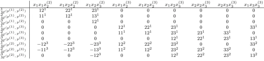
Example B.1 Letc=x1x2,d=x2x3 ande=x3x3 be the monomials we removed (see Sect. 3). Note,
asx3x1x2=x1x2x3we need a third monomialx3x3to remove the correct number of (linearly dependent)
equations. Obviously1216= 0is a necessary conditions for table 6 to be regular. Thus the rst 3 rows are
Table 6: Matrix of destroyed systematic dependencies.
x1x1x (2)
2 x1x2x (2)
2 x1x2x (2)
3 x1x1x (3)
2 x1x2x (3)
2 x1x2x (3)
3 x2x2x (3)
3 x2x3x (3)
3 x1x3x (3) 3
πM1 (p(1), p(2) ) 121 221 231 0 0 0 0 0 0 π2
M(p(1), p(2) ) 111 121 131 0 0 0 0 0 0
π3
M(p(1), p(2) ) 0 0 121 0 0 0 0 0 0
π1
M(p(1), p(3) ) 0 0 0 12
1 221 231 0 0 331
π2
M(p(1), p(3) ) 0 0 0 111 121 231 231 331 0
π3
M(p(1), p(3) ) 0 0 0 0 0 121 221 231 131
π1
M(p(2), p(3) ) −123 −223 −233 122 222 232 0 0 332
π2
M(p(2), p(3) ) −11
3 −123 −133 112 122 232 232 332 0
π3
M(p(2), p(3) ) 0 0 −123 0 0 122 222 232 132
linearly independent with probability 1−1
q
2
. After Gaussian Elimination the remaining lower right
(3×3)-submatrix do not contain systematic zeros or dependencies and thus the overall probability of 6
to be regular is
2
Q
i=0
(q3−qi)
q9
1−1
q
2
. (22)
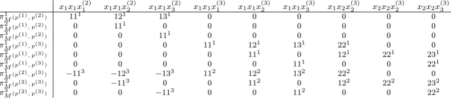
Example B.2 Letc=x1x1andd=x2x2 be the monomials we remove (see Sect. 3). Obviously1116= 0
and (221∨222) 6= 0 are necessary conditions for table 7 to be regular. This holds with probability
1−1
q 1−
1
q2
. The rst six lines are now linearly independent and after Gaussian Elimination the lower right3×3submatrix is of the following shape, where white stand for zero, gray for some entry and
xfor the same entry:
x x
The probability of this matrix to be regular is 1−1
q
2
and thus the overall probability is
1−1
q
3
1− 1
q2
Table 7: Matrix of destroyed systematic dependencies.
x1x1x(2)1 x1x1x(2)2 x1x1x(2)3 x1x1x(3)1 x1x1x(3)2 x1x1x(3)3 x1x2x(3)2 x2x2x(3)2 x2x2x(3)3
πM1 (p(1), p(2) ) 111 121 131 0 0 0 0 0 0 π2
M(p(1), p(2) ) 0 111 0 0 0 0 0 0 0
π3
M(p(1), p(2) ) 0 0 111 0 0 0 0 0 0
π1
M(p(1), p(3) ) 0 0 0 111 121 131 221 0 0
πM2 (p(1), p(3) ) 0 0 0 0 111 0 121 221 231 π3
M(p(1), p(3) ) 0 0 0 0 0 111 0 0 221
π1
M(p(2), p(3) ) −113 −123 −133 112 122 132 222 0 0
π2
M(p(2), p(3) ) 0 −113 0 0 112 0 122 222 232
πM3 (p(2), p(3) ) 0 0 −113 0 0 112 0 0 222
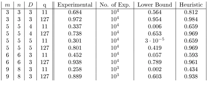
To study the behavior of our algorithm we rst give a lower bound on the probability of success. This bound is bad in some cases (cf. table 8) and thus we secondly give a expected probability of success by using a heuristic.
As in equation (19) our algorithm destroy all systematic dependencies. For D > 2 we derive the
same matrix as in (4), but with blocks of a larger size si. Due to our algorithm the i-th block still is
a submatrix of the upper left part of the block i+ 1(see gure 1). If block iis regular we can remove
Figure 1: Blockwise dependence of regularity.
i i
i+ 1
the rstscolumns in the rstsrows of blocki+ 1by Gaussian elimination. Thus block i+ 1is regular
i the obtained block of size (si+1×si+1) is regular (see gure 1). Unfortunately we cannot assume
the elements of a single block to be uniformly random. Depending on the choice of monomials of Mon2
there could be strong dependencies among the elements, especially for blocks with smalli(see App. B.1,
Tab. 6 for examples). We can derive the sizesi directly from algorithm 2 and formulate the following
corrolary.
Corollary B.3 LetD= 2k+b withb∈ {0,1} be the solving degree of XL and
zi:=
n+D −3
D−2
+
min{i−1,k−1}
X
j=1
(−1)j
n+D
−3−2j D−2−2j
i −1
j
| {z }
:=τij
. (24)
The size si of thei-th block of matrix M with 1≤i≤m−1is given by
si=si−1+zi withs1:=z1=
n+D −3
D−2
.
In order to determine the behavior of our algorithm we give a lower bound of the probability of success.
Lemma B.4 Let m, n > 1 be the number of equations respectively variables of an uniformly random
MQ-system, D the solving degree of XL and zi as dened in corollary B.3. A lower bound for the
probability of success of algorithm 2 is given by
1−1
q
Pmi=1−1zi
Algorithm 5 Generating linearly independent equations(D= 2)
1: eqn← {}; miniList←Mon2;
2: fori:= 1tomdo
3: forµ∈miniList do 4: eqn←eqn∪ {µp(i)};
5: if |eqn|=T−D−2 then
6: Stop;
7: end if 8: end for 9: η∈RminiList;
10: miniList←miniList\{η}; 11: end for
Proof. Let M be the matrix given the rowsπk M(p
(i), p(j))with a xed setAof elements that are zero
and a xed set B of the remaining elements, i.e. |A|+|B|=z2 withs
1 (see corollary B.3) the size of
the rst block in M. All the elements of B are chosen uniformly random. We observe the probability
space of all matrices M such that the probability of being regular is not zero. Note that matrix M has no systematic dependencies between the rows, i.e. for some choice of elements it has to be regular. The worst case structure of a matrix M regarding the probability of being regular, is an upper (or lower) triangular matrix. The probability of such a (s1×s1)matrix to be regular is the probability of
every diagonal element to be dierent from zero, i.e. 1−1
q
s1
. Obviously this probability gets better if we introduce dependencies between variables. If for example x1 =x2 then the probability raise to
1−1
q
s1−1
. It can be easily shown by induction that the probability of success also increase if we increase the number of elements inB, i.e. if we destroy the triangular structure. As we havem−1such
matrices of sizezi for1≤i≤m−1to be regular, equation (25) is a lower bound for the probability of
success.
Table 8: Comparison experimental success probability, lower bound and heuristic.
m n D q Experimental No. of Exp. Lower Bound Heuristic
3 3 3 11 0.684 104 0.564 0.812
3 3 3 127 0.972 104 0.954 0.984
5 5 4 11 0.337 104 0.006 0.659
5 5 4 127 0.738 104 0.653 0.969
5 5 5 11 0.301 104 3·10−5 0.659
5 5 5 127 0.801 104 0.419 0.969
6 6 3 11 0.452 104 0.057 0.593
6 6 3 127 0.938 104 0.789 0.961
9 8 3 11 0.258 103 0.002 0.434
9 8 3 127 0.889 103 0.603 0.938
Table 8 shows that (25) is a quite bad bound in some case. The proof of lemma B.4 suggests that for largen,mandDthei-th block of matrix M, precisely the lower right(zi×zi)submatrix after Gaussian
Elimination, is a random matrix and not, as for the lower bound assumed, a triangular matrix. This leads to the following heuristic.
Heuristic. For largen,mandD the probability of success of algorithm 2 is close to
m−1
Y
i=1
zi−1 Y
j=0
For real worldMQ-systems, such as UOV withm= 26, n= 24, q= 256andD= 12the lower bound
is almost0. The heuristic tells us that our algorithm should succeed with probability 0.901. Clearly it
![Table 1: HybridF5variables overset inregularity for FSmall Linearization ( (H5) from [BFP09], plain XL (Alg](https://thumb-us.123doks.com/thumbv2/123dok_us/1875514.1244196/12.595.129.466.263.571/table-hybridf-variables-overset-inregularity-fsmall-linearization-plain.webp)
![Table 2: Comparison between Small Linearization (shave guessℓ) and HybridF5 (H5)from [BFP09]](https://thumb-us.123doks.com/thumbv2/123dok_us/1875514.1244196/13.595.132.464.124.247/table-comparison-small-linearization-shave-guess-hybridf-bfp.webp)