$HB^N$: An HB-like protocol secure against man-in-the-middle attacks

HB

N

: An

HB-like protocol secure against man-in-the-middle attacks

Carl Bosley

Kristiyan Haralambiev

Antonio Nicolosi

August 5, 2011

Abstract

We construct a simple authentication protocol whose security is based solely on the problem of Learning Parity with Noise (LPN) that is secure against Man-in-the-Middle attacks. Our protocol is suitable for RFID devices, whose limited circuit size and power constraints rule out the use of more heavyweight operations such as modular exponentiation. The protocol is extremely simple: both parties compute a noisy bilinear function of their inputs. The proof, however, is quite technical, and we believe that some of our technical tools may be of independent interest.

1

Introduction

Motivation. Many cryptographic tasks originate from the necessity to reproduce in cyber space security properties that exist in the physical world. Examples in point include digital signatures (non-repudiation) or public-key encryption (drop-boxes). Among the basic cryptographic goals, authentication has the potential to straddle the physical and cyber world, and enable authentication cryptographically strong authentication of physical things.

For moderately powerful devices like smartphones, or even battery-operated sensors, existing authentication protocols often suffice. Computationally weak devices such as RFID devices and batteryless contactless smartcards, however, require more lightweight, dedicated solutions.

RFID devices are quickly becoming popular in many applications. They are used throughout the supply chain for inventory management. RFID can be used to replace physical keys for access control. Banking and financial institutions have also started to embrace them for account management. Mass transit authorities in several metropolitan areas have taken to used them to replace tokens; similarly, RFID-mediated access to toll roads is the norm all over the world.

RFID devices can do all this, silently. Unfortunately, this silence leaves them vulnerable to stealth queries from malicious entities. This introduces an array of security risks, including unauthorized access, fraudulent account usage, as well as privacy risks, such as stealth tracking.

Learning parity with noise. TheLPNproblem was introduced in the machine learning community by Angluin and Laird [AL87]. It soon became notorious for having no efficient noise-tolerant algorithm. It was proven by Kearns [Kea93] that the class of noisy parity concepts (LPN) is not learn-able within the statistical query model. Work onLPN-based protocols began with theHB protocol of Hopper and Blum [HB01], which was later proven to be secure againstPassive

attacks assuming the hardness ofLPN.

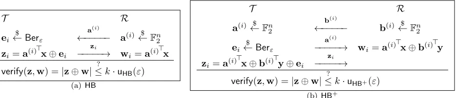
HB-type protocols. The original motivation for theHBprotocol was to enable unaided human authentication: the goal was for the protocol to be simple enough to be carried out without the help of a computational device. Subsequent work has found that the key sizes and error rates required to ensure security may be too large for humans to employ with ease comparable to, say, password-based authentication. Nevertheless, as noted by Juels and Weis [JW05], HB-type protocols are lightweight enough to be potentially applicable in the RFID setting. Indeed, constraints on power consumption and circuit size (1,000–4,000 transistors) for RFID devices makes it problematic to deploy conventional cryptographic algorithms like AES or modular exponentiation on these devices;HB-type protocols, on the other hand, have very simple circuit representations. For example, the interaction between the prover, or tag T, and the verifier, or readerR, in the

HB protocol consists of two messages: first,R sends a random challengea∈F2n. Next, T samples e∈ F2 according to

the Bernoulli distributionBerε (i.e. Pr[e= 1] =ε). T sendsz=a>x+e toR, wherex∈Fn2 is a key shared between T

and R. Raccepts ifz=a>x. The basic protocol has soundness 1₂ and completeness 1−ε, but this can be improved via sequential or parallel composition (cf. Section 2.3).

∗_{Dept. of Computer Science, Stevens Institute.[email protected].} †_{Dept. of Computer Science, New York University.}

[email protected]. ‡_{Dept. of Computer Science, Stevens Institute.}

In [JW05], Juels and Weis also introduced HB+, which was shown to be secure in a slightly stronger security model (known as Activesecurity) than the original HBprotocol. Gilbert, Robshaw, and Seurin ([GRS05]) showed thatHB+ is vulnerable to a man-in-the-middle attack. A number of variants of HB+ _{were proposed to remedy this defect, including} HB++ [BCD06], HB∗ [DK08], HB-MP [MP07], HB-MP’ [LMM08], and Trusted-HB [BC08]. However, all of these were proven insecure. Gilbert, Robshaw, and Seurin ([GRS08a]) extended their attack onHB+ _{to breakHB}++_,HB∗

,HB-MP,

HB-MP’, and Frumkin and Shamir [FS09] showed that Trusted-HBis insecure.

Gilbert, Robshaw, and Seurin [GRS08b] introduced HB#_{, which was secure against the same attack that succeeded}

againstHB+. However, Oaufi et al [OOV08] presented anMan-in-the-Middleattack onHB#.

Katz, Shin, and Smith [KSS10] provided the first proof of security forHBandHB+ _{for any error rateε <1/2, via black}

box reductions. However, forHB+ the reduction used rewinding, so that it achieved active security √ε assumingLPNis hard for noise rateε.

Pietrzak then introduced Subspace LWE [Pie10], a more flexible formulation ofLPNthat is nevertheless equivalent to

LPN. In a major advance, Kiltz et al. [KPC+11] built on Subspace LWE [Pie10] to construct a two-round Active-secure protocol, as well as two secure MACs, which imply two-roundMan-in-the-Middle-secure protocols. However, both Man-in-the-Middle-secure constructions require the use of an (almost) Pairwise Independent Permutation on approximatelyO(n2) bits. Furthermore, the first MAC’s security reduction is loose, achieving security √ε, while the second construction is much more complicated and requires a longer key.

1.1

Our Contribution

Our protocol, like the originalHBprotocol, is extremely simple: instead of computing a noisy linear functiona>x+e, the parties compute a noisybilinearfunctiona>Xb+eof their joint inputsa,b. As described in Section 3, this can be done in either 2 or 3 rounds.

However, the Man-in-the-Middlesecurity proof is quite technically involved, particularly in the understanding of the noise distributions. We develop some technical tools, including theLSN(Learning Subspaces with Noise) problem, which we believe will be of independent interest.

Another new technique that may be useful elsewhere is the probabilistic scheme for the Verifier, which was not present in earlier protocols. Our Verifier simply adds noise mirroring the noise from the Tag. This eliminates a major difficulty in earlier protocols, for which deterministic verification was often exploited to design attacks.

Interestingly, although its simplicity was obscured by notation, a similar bilinear protocol was proposed in Section 5.2 of [KPC+11] and proven to beMan-in-the-Middle-secure. However, [KPC+11] used more heavyweight tools such as Waters’ technique for converting a selectively secureMACto a fully secureMAC.

1.2

Outline

We describeLPN,HBandHB+_{, and thePassive,Active, andMan-in-the-Middlesecurity models in Section 2. In Section 3,}

we describe the HBN protocol family. In order to analyze the security of HBN, we first need to develop new tools for precisely manipulating error distributions, including theLSN(Learning Subspaces with Noise) problem, which we present in Section 4. Finally, in Section 5, we prove thatHBN_{is secure againstMan-in-the-Middleattacks.}

2

Preliminaries

2.1

Notation

We writex←$ X to denote the process of assigning a value sampled from the distributionX to the variablex. IfS is a finite set, we write s←$ S to denote assignment tos of a value sampled from the uniform distribution onS. We use [n] to denote the set {1,2, . . . , n}. Vice versa, we will abuse set-notation to identify a distributionX with its support; for example, we writex∈X to denote thatxis in the support ofX. IfAis a probabilistic algorithm, we letA(x) denote the output distribution of Aon inputx, and writey← A$ (x) to denote the process of running algorithm Aon inputxand assigning its output toy. We write:

Pr[x1 $ ←X1, x2

$

←X2(x1), . . . , xn $

←Xn(x1, . . . , xn−1) :φ(x1, . . . , xn)]

to denote the probability that the predicateφ(x1, . . . , xn) is true, when for all i∈[n],xi is drawn from distributionXi,

possibly depending on the values drawn forx1, . . . , xi−1. Whenn= 1, ˆx∈X1, andφ(x1) is of the form “x1 = ˆx1”, we use

the shorthand Pr[ˆx1 $

←X] to denote Pr[x1 $

←X1 :x1 = ˆx1]. For two probability distributionsX1, X2, we writeX1≡X2

if and only if∀ˆx∈X1∪X2,Pr[ˆx $

LetFqrepresent the finite field withqelements. We denote the uniform distribution overFn2 byUn×n, and the Bernoulli

distribution with biasεbyBerε. (Recall thatBerεis the distribution overF2 with Pr[1 $

←Berε] =ε, Pr[0 $

←Berε] = 1−ε.)

We use the binary operator ⊕:F2×F2 →F2 to represent finite field addition, and forb∈ F2, we let b= 1⊕b be the

complement ofb. For an eventS,S represents its complement, the event thatS does not occur.

We denote column vectors by lower-case bold letters such asx, and matrices by upper-case bold letters such asX. We denote the transpose ofXbyX>. For a matrixA∈F2m×n,rank(A) denotes the rank ofA. ker(A) ={x:Ax= 0}denotes

the kernel ofX, the set of all vectors orthogonal toA, andIm(A) ={y:∃xs.t.Ax=y}denotes the image ofA, the set of all linear combinations of columns ofA. Indenotes then×nidentity matrix.

We will often consider column vectorsx,y∈F`2as matrices inF`

×1

2 . Consideringx,y as matrices allows us to extend

operations on matrices to vectors. For example, we can form the outer product xy>∈F`2×`, and form the kernel ker(x).

The dot product of two column vectors x,y can be written as the matrix multiplicationx>y. For a vectorx, we denote the scalari-th element ofxbyxi. 0ndenotes the all-zero column vector of lengthn. e(i,`)∈F`2 denotes thei-th vector of

the canonical basis, for whiche(i)_i = 1, ande(i)_j = 0 forj6=i. In practice, when the dimension can be determined from context, we drop it, lettinge(i)_=e(i,`)_{. For a vectorx, let|x|denote the number of nonzero entries ofx.}

We denote an arbitrary polynomial function of n bypoly(n). We write f = negl to mean that f is negligible as a function ofn, that is,f=o(n−c_{) for any constantc >0.}

2.2

Learning Parity with Noise (

LPN

)

Roughly speaking, the problem of Learning Parity with Noise amounts to distinguishing two distributions over Fn2 ×F2:

the uniform distribution and theLPN distribution. For a random secret vector x∈ Fn2, theLPN distribution is in turn

defined in terms of its sampling algorithm LPNxε, shown in Algorithm 2.2. AlgorithmLPNxε is initialized with a uniform

secret vector x ←$ Fn2. Thereafter, whenever an LPN sample is requested, the algorithm chooses random a $

← Fn2 and

e←$ Berεand outputs (a, b), whereb=a>x⊕e. Forε=1₂,LPNbecomes the uniform distribution.

1: functionLPNx ε

2: a←$ Fn2

3: e←$ Berε

4: b=a>x+e 5: return(a, b)

Algorithm 1: LPN

We will use the decisional version of theLPNhardness assumption, which is defined using an indistinguishability game. It has been shown [KSS10] that hardness of the decisional version is equivalent (up to polynomial factors) to hardness of recovering the entire key. The decisional variant ofLPN is hard if it is difficult to distinguish between an oracle with distribution LPNx

ε versus an oracle with a random distribution Un×U1, which (by Corollary 8) can be represented as LPNx1/2. More formally, the advantage of an algorithmAagainstLPNfor a given (ε, n) is defined using a game in which

the adversary attempts to guess which oracle was selected:

Definition 1. The decisionalLPNassumption states that for all efficient adversariesA,AdvLPNA (ε, n)≤εLPN=negl, where

AdvLPN

A (ε, n) is defined as

AdvLPNA (ε, n) =

Pr 

   

x←$ Fn2, b $ ←F2, Ob=

LPNx1/2 if b= 0 LPNxε, if b= 1

,

ˆ

a← A$ Ob₍₁n₎

: ˆa=b 

   

−1

2

(1)

2.3

HB

and

HB

_protocols

TheHB,HB+_{protocols consist ofk=poly(n) iterations of what is known as a “basic authentication step”. The protocols}

are executed by two parties: the tagT, who wishes to authenticate, and the readerR, who verifies the tag. 1 The key for

HBis a vectorxof lengthn, wherenis the security parameter. ForHB+_{, the key consists of two vectorsx,yof lengthn.}

to the tag, and the tag replies withzi=a(i)

>

x⊕ei, whereei $

←Berε. HB+ adds a second secretyand a third round, as

shown in Figure 1(b).

In bothHBandHB+_{, at the end ofkrounds,Rchecks to see what fraction of answersz}

i were correct. If more than

k·u(ε) are correct, for u(ε) some function ofε, thenverify(z,w) returns true, and the reader accepts. Otherwise, the reader rejects. kandu(ε) should be set high enough to allow the honest tag to authenticate w.h.p., but low enough that a malicious third party should not be able to authenticate by randomly guessing. In particular, as noted in [KSS10], for both

HBand HB+_{,u(ε) = (1 +δ)ε suffices to achieve completeness error negligible in the security parameter, for any positive}

constantδ.

T R

ei

$

←Berε

a(i)

←−−−−− a(i)_←$

Fn2

zi=a(i)

>

x⊕ei

zi

−−−−−→ wi=a(i)

>

x

verify(z,w) =|z⊕w|≤? k·uHB(ε) (a) HB

T R

a(i)_←$

Fn2

b(i)

←−−−−− b(i)_←$

Fn2

ei

$

←Berε

a(i)

−−−−−→ wi=a(i)

>

x⊕b(i)>_y

zi=a(i)

>

x⊕b(i)>y⊕ei

zi −−−−−→

verify(z,w) =|z⊕w|≤? k·uHB+(ε) (b)HB+

2.4

Security Models

In this subsection we present several natural security models that have been used for authentication and for HB-type protocols in particular. The more general models arePassive,Active, andMan-in-the-Middle. Additionally, several works have used an intermediate model, GRS-MIM, which is stronger than Active yet weaker than the full Man-in-the-Middle

model.

Passive Model: In Phase I, the attacker can only observe the interactions betweenT andR.

ActiveModel: In Phase I, as shown in Figure 1, the tag interacts with the attacker, who is free to choose non-random a. However,bremains randomly chosen. Note that the attacker does not have access to a reader, and thus is unaware of the results of the reader’s verification step.

T A

b(i)

−−−−−→

a(i)

←−−−−−

zi −−−−−→

(c) Three Rounds

T A

a(i)

←−−−−−

b(i),zi −−−−−→

(d) Two Rounds

Figure 1: Active

T A R

b(i)

−−−−−→ b

0(i) −−−−−→

a0(i)

←−−−−− a

(i) ←−−−−−

zi −−−−−→

z0_i

−−−−−→ wi =. . .

verify(z,w) =|z⊕w|≤? k·u(ε)

(a) Three Rounds

T A R

a0(i)

←−−−−− a

(i) ←−−−−−

b(i),zi −−−−−→

b0(i),z0_i

−−−−−→ wi=. . .

verify(z,w) =|z⊕w|≤? k·u(ε)

(b) Two Rounds

Figure 2: Man-in-the-Middle

GRS-MIM Model: TheGRS-MIMmodel of Gilbert, Robshaw, and Seurin [GRS08b] is a variant of the Man-in-the-Middle model, in which the adversary is not allowed to modify zi. That is, ∀i,zi = z0i. GRS-MIM includes the attack

onHB+_{, so thatHB}+ _{is not secure in theGRS-MIM model. The restrictionz}

i =z0i is unrealistic in practice, but GRS-MIM was used by a number of recent works in an attempt to improve on HB+, due to the difficulty of proving security in the fullMan-in-the-Middlemodel. However,GRS-MIM-security does not implyMan-in-the-Middle-security, and indeed,

GRS-MIM-secure protocols have been successfully attacked in the full model [OOV08].

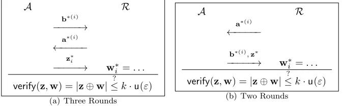
Phase II. In all three models, the goal of the attackerA is to authenticate successfully to the readerRinkrounds of Phase II, as shown in Figure 3. A is successful iffverify(z) returnstrueandb∗6=0in allkrounds.

A R

b∗(i)

−−−−−→

a∗(i)

←−−−−−

z∗_i

−−−−−→ w_i∗=. . .

verify(z,w) =|z⊕w|≤? k·u(ε)

(a) Three Rounds

A R

a∗(i)

←−−−−−

b∗(i)_,z∗

−−−−−→ w_i∗=. . .

verify(z,w) =|z⊕w|≤? k·u(ε)

(b) Two Rounds

Figure 3: Phase II (All Models)

3

Our protocol

We present theHBN _{protocol, in 2-round and 3-round variants. Our secret key will be a matrixX ∈}

Fn2×n. As before,

a(i),b(i)∈Fn2 are column vectors used in the execution. The protocol consists of the key generation stepKeyGenand the

authentication stepAuth.

KeyGen. KeyGen(1n_{) produces a matrixX} $ ←Fn2×n.

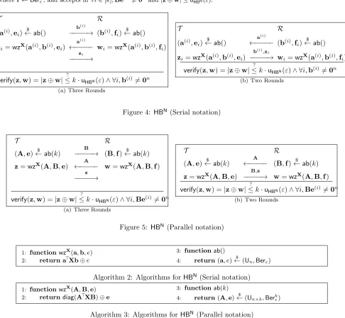
Auth. HBN_{can be run in serial or in parallel. We describe the serial version first, and then modify the notation for the} parallel version. The tag TX

ε = (Tb(),TzX(·,·,·)) authenticates to the readerRXε = (Ra(),RwX(·,·,·)) by performing k

rounds of the protocol, as shown in Figure 4. LetRa() =Tb() =ab(), andRw(·,·,·) =Tz(·,·,·) =wz(·,·,·), as shown in Algorithm 2.

In each of k rounds, which can be executed in serial or in parallel, Tε(X) draws (b(i),fi) $

← Tb(), while R draws (a(i),ei)

$

←Ra().T sendsb(i)toR, whileRsendsa(i)toT. This can be done in either order: ifT sends first, the protocol becomes 3 rounds, while ifRsends first, the protocol becomes 2 rounds. Finally,Tε(X) computeszi=TzX(a(i),b(i),fi)

and sends toRX

what fraction of responses were correct. Ralso tests to ensure that ∀i∈[k],b(i) 6=0n. If allb(i) are nonzero and more thank·uHBN(ε) =k(1 +δ)(ε⊕ε) for some completeness parameterδ, the reader accepts. 2

Parallel version. We can use matrix notation to simplify working with HBN _{in parallel, as shown in Figure 5 and} Algorithm 3. Let A,B∈ F2n×k be matrices for which∀i∈[k],Ae

(i)

=a(i),Be(i) =b(i). That is, the columns ofA,B respectively are the vectors a(i)_,b(i) _{respectively. Then in the two-round version, for example, R sends the challenge}

A←$ Fn2×k. T replies with B $

←Fn2×k andz=diag(A

>

XB)⊕e, wheree←$ Bern

ε. Rcomputes w=diag(A

>

XB)⊕f, wheref ←$ Bernε, and accepts iff∀i∈[k],Be(i)6=0nand|z⊕w| ≤uHBN(ε).

T R

(a(i)_,e

i)

$

←ab()

b(i)

−−−−−→ (b(i)_,f

i)

$

←ab()

zi=wzX(a(i),b(i),ei)

a(i)

←−−−−− wi=wzX(a(i),b(i),fi)

zi −−−−−→

verify(z,w) =|z⊕w|≤? k·uHBN(ε)∧ ∀i,b(i)6=0n

(a) Three Rounds

T R

(a(i)_,e

i)

$

←ab()

a(i)

←−−−−− (b(i)_,f

i)

$

←ab()

zi=wzX(a(i),b(i),ei)

b(i)_,z i

−−−−−→ wi=wzX(a(i),b(i),fi) verify(z,w) =|z⊕w|≤? k·uHBN(ε)∧ ∀i,b(i)6=0n

(b) Two Rounds

Figure 4: HBN _{(Serial notation)}

T R

(A,e)←$ ab(k)

B

−−−−−→ (B,f)←$ ab(k)

z=wzX_{(A,B,e) ←−−−−−}A _w=wzX_(A,B,f) z

−−−−−→

verify(z,w) =|z⊕w|≤? k·uHBN(ε)∧ ∀i,Be(i)6=0n

(a) Three Rounds

T R

(A,e)←$ ab(k)

A

←−−−−− (B,f)←$ ab(k)

z=wzX_{(A,B,e) −−−−−→}B,z _w=wzX_(A,B,f)

verify(z,w) =|z⊕w|≤? k·uHBN(ε)∧ ∀i,Be(i)6=0n

(b) Two Rounds

Figure 5: HBN_{(Parallel notation)}

1: functionwzX(a,b, e) 2: return a>Xb⊕e

3: functionab()

4: return(a, e)←$ (Un,Berε) Algorithm 2: Algorithms forHBN(Serial notation)

1: functionwzX(A,B,e) 2: returndiag(A>XB)⊕e

3: functionab(k)

4: return(A,e)←$ (Un×k,Berkε) Algorithm 3: Algorithms forHBN (Parallel notation)

4

Learning Subspaces with Noise (

LSN

)

Outline. In this section, we present a new conceptual tool in for analyzing HB-like protocol, theLSN(Learning Subspaces with Noise) problem, as shown in Algorithm 4.3. The security ofLSNis equivalent to that ofLPN. First, in Section 4.1, we introduce a new (to our knowledge) compact notation for precisely working with sums of random variables overF2, in

order to simplify working withLPN andLSN. Next, in Section 4.2, we establish several fundamental properties of LPN. We work withLSNitself in Section 4.3.

4.1

Working with probability distributions of additive variables over

_F

We will need to analyze sums of noise distributions. Our task will be made easier by the use of a compact and flexible notation describing our distributions. At the most basic level, we need to understand the sum of two different Bernoulli distributions,Berδ⊕Berγ. Intuitively, noise is additive, and bounded above byδ+γ. However, it is also possible for errors

to cancel. Indeed,

Pr[1←Berδ⊕Berγ] = Pr[1←Berδ∧0←Berγ] + Pr[0←Berδ∧1←Berγ]

=δ(1−γ) +γ(1−δ) =δ+γ−2γδ (2)

We would like to define an operator that adds these distributions, in the same sense that ⊕is the additive operator overF2. We can describe each distributionX by a single scalar,δX = Pr[X= 1], withδXan element of the closed interval

[0,1]. So, given⊕:F2×F2→F2, we define an induced operator⊕∗: [0,1]×[0,1]→[0,1] which adds distributions: Berγ⊕∗_δ=Ber_γ⊕Ber_δ

It follows from Equation 2 that for all γ, δ∈ [0,1], ⊕∗ must satisfy γ⊕∗δ =δ+γ−2γδ. This is sufficient to uniquely define the operator. ⊕∗

acts similarly to the familiar binary operator⊕: it is associative, commutative, and obeys the equalities 0⊕∗x=xand 1⊕∗x= 1−xfor allx∈[0,1]. For this reason, we drop the∗and simply refer to our operator as⊕. We also observe that we can extend the complement operator·to all of [0,1], so that for allδ∈[0,1],δ= 1⊕δ. In summary, we have defined⊕,·so that

∀δ∈[0,1], δ= 1. ⊕δ= 1−δ

∀γ, δ∈[0,1], γ⊕δ=. δ·γ+δ·γ= (1−δ)γ+ (1−γ)δ=γ+δ−2γ·δ (3)

Other useful facts about⊕over [0,1] that we will use in the following are: Fact 2. ∀ε∈[0,1],1

2⊕ε= 1 2.

Fact 3. ∀ˆ_b∈F2,Pr[e $

←Berε:e= ˆb] = ˆb⊕ε=

(

ε ifˆb= 1

1−ε ifˆb= 0 .

The presence of the complement operator is due to the convention of parameterizing the Bernoulli distribution by Pr[Berε= 1] =ε. If Pr[Berε= 0] was used instead, we would obtain the simpler expression ˆb⊕ε. For this reason, we have

chosen to complement the error termεrather than the desired bit ˆb.

Fact 4. Letε⊕n=

n

z }| {

ε⊕ε⊕. . .⊕ε. Thenε⊕n= 1−(1−₂2ε)n.

Fact 4 tells us that noise behaves multiplicatively rather than additively. The reason it appears additive for small noise rates corresponds to the approximation exp(x)≈1 +xfor small x. More precisely, the scaled distance from 1

2 behaves

multiplicatively:

Fact 5. For allδ, τ∈[0,1], 1₂(1−δ)⊕1

2(1−τ) = 1

2(1−δτ).

4.2

Learning Parity with Noise (

LPN

)

Next we establish a characterization of theLPNdistribution in Lemma 6 and examine its consequences.

Lemma 6. ∀(ˆa,ˆb)∈Fn2 ×F2,Pr[(ˆa,ˆb)←LPNxε] = (ˆa>x⊕ˆb⊕ε)2−n=

(

ε2−n ifaˆ>x6= ˆb (1−ε)2−n ifaˆ>x= ˆb.

Proof. Sincea, eare chosen independently, we have:

Pr[(ˆa,ˆb)←LPNxε] = Pr[(a, b)←LPN x

ε :a= ˆa]·Pr[e←Berε:e= ˆa

> x⊕ˆb]

= Pr[ˆa←$ Fn2]·Pr[e←Berε:e= ˆa

> x⊕ˆ_b]

= 2−n(ˆa>x⊕ˆb⊕ε) (4)

Equation 4 follows from Fact 3.

Summing over all ˆa∈Fn2 yields the following corollary:

Corollary 7. ∀x6=0n, Pr[(a, b)←LPNxε :b= 0] = 1₂.

Settingε=1

Corollary 8. Pr[(ˆa,ˆb)←LPNx1/2] = 2

−n−1

. Equivalently,LPNx1/2 ≡Un×U1.

Finally, a useful consequence of the random self-reducibility properties of the LPN problem is that, given anyLPN

distribution for any fixed keyx, we can produce anLPNdistribution with a random key and the sameε:

Corollary 9. For any ε ∈ [0,1] and x,y ∈Fn2, the distribution LPNxε⊕y can be efficiently sampled given y and oracle

access toLPNx ε.

Proof. Consider the “translated” distribution Tr-LPNxε defined as follows: draw a sample (a, b) from LPNxε, and return

(a, b⊕a>y). Then:

Pr[(ˆa,ˆb)←Tr-LPNxε] = Pr[(ˆa,ˆb⊕ˆa

>

y)←LPNxε]

= 2−n(ˆa>x⊕aˆ>y⊕ˆb⊕ε) = Pr[(ˆa,ˆb)←LPNxε⊕y]

Corollary 9 says that we can “duplicate” anLPN distributionLPNx

ε: we can use some of its samples as is, from the

original distribution, and at the same time use the remaining samples as if they came from an entirely different LPN

distribution with the sameε(even for unknownε). Furthermore, if the “translation” vector yis uniformly random, then the originalLPNdistributionLPNxε and its “translate”LPNxε⊕yare independent.

Lemma 10. Given a challenge oracleOb= (

LPNr1/2 if b= 0 LPNrε, if b= 1

, we can construct`separate challenge oracles,(O(1)b , . . . ,O (`) b ) =







(LPNz1/2(1), . . . ,LPN z(`)

1/2) if b= 0

(LPNzε(1),LPN z(`)

ε ) if b= 1

Proof of Lemma 10. Lety(i) $

←Fn2,∀i∈[`]. Repeated applications of Corollary 9 yield new oracles (LPNz (1)

ρ , . . . ,LPNz (`) ρ ),

where z(i)=y(i)⊕r. Since thez(i) are independently and uniformly distributed for alli∈[`], and sinceρ=1₂ forb= 0 andρ=εforb= 1, this establishes the lemma.

4.3

Learning Subspaces with Noise (

LSN

)

Next, we introduceLSNxρ,ε, which usesLPNxε to produce a biased halfspace distribution: ais chosen randomly subject to the

condition thata>xis distributed according toBerρ⊕Berε. In particular, forLSNx0,ε,a

>

x≡Berε. We derive an expression

for the distribution of (a, b)←$ LSNxρ,εin Lemma 12 intermediate results. We consider the caseε=12 in Corollary 13. Next

we consider the conditional distribution of b given a>x = ˆa in Corollary 15. Finally, we establish a connection between hardness ofLSNx

ρ,ε andLPNxε.

1: functionLSNxρ,ε

2: returnLSNρ(LPNxε)

3: functionLSNρ(Samp)

4: i= 0 5: ˆb←$ Berρ

6: repeat

7: (a(i), bi) $

←Samp() 8: i←i+ 1

9: untilbi= ˆb

10: return(a(i), bi)

Algorithm 4: LSN

The algorithmLSNx

ρ,ε, shown in Algorithm 4.3, is constructed from the oracleLPNxε. LSNxρ,εfirst uses its own

random-ness to draw ˆb←$ Berρ. Next, fori≥0 it repeatedly obtains (a(i), bi) $

←LPNxε. The algorithm waits untilbi= ˆb, and then

outputs (a(i)_{, b}

i). The algorithm runs in expected polynomial time.

The distribution of (ˆa,b)ˆ ←$ LSNxρ,εcan be computed fromρand the distribution of (ˆa,b)ˆ $

Lemma 11. Pr[(ˆa,ˆb)←$ LSNxρ,ε] = 2 Pr[ˆb $

←Berρ]·Pr[(ˆa,ˆb) $ ←LPNxε].

Proof of Lemma 11. The algorithmLSNxρ,εprogresses through a series of rounds. In each round,LSNρ,εsamples (a(i), bi) $ ← LPNx

ε. The algorithm terminates by returning (a(i), bi) when it findsbi= ˆb. To model its distribution, we define a series

of events. Let Rˆb be the event that ˆb=bi. LetS (i)

be the event that, given that the algorithm is active during roundi,

the algorithm terminates by returning (a(i)_{, b}

i) in roundi, fori≥0. Finally, letT (i)

(ˆa,ˆb) be the event that (ˆa,

ˆ

b)←$ LPNx ε in

roundi. It follows that

Pr[(ˆa,ˆb)←$ LSNxρ,ε] =

∞

X

i=0

Pr[S(i)]Y

j<i

Pr[S(j)_]

!

Pr[Rˆb]·Pr[T (i) (ˆa,ˆb)]

(5)

= ∞

X

i=0

1 2

i

Pr[ˆb←$ Berρ]·Pr[T (i) (ˆa,ˆb)]

(6)

= (ˆb⊕ρ) ∞

X

i=0

1 2

i

Pr[T(i)

(ˆa,ˆb)]

(7)

= 2(ˆb⊕ρ)·Pr[T(0)

(ˆa,ˆb)] (8)

Equation 5 follows from summing over alli≥0 and all bits ˆb∈F2 the probability that LSNxρ,ε terminates in round

i with output (ˆa,ˆb). Equation 6 follows from Corollary 7 and from the definition ofLSN in Algorithm 4.3. Equation 7 follows from Fact 3. Equation 8 follows from the geometric series formula and from∀i,Pr[T(i)

(ˆa,ˆb)] = Pr[T (0) (ˆa,ˆb)].

Next, we apply Lemma 6 to derive the probability distribution ofLSN.

Lemma 12. For allaˆ∈Fn2,aˆ∈F2,ˆb∈F2,

(a) Prh(ˆa,ˆb)←LSNx ρ,ε

i

= (ˆb⊕ρ)(ˆb⊕ˆa>x⊕ε)2−n+1

(b) Pr

(a, b)←LSNxρ,ε: ˆa=a

= (ˆa>x⊕ρ⊕ε)2−n+1

(c) ∀x6=0n_,Prh_{(a, b)←LSN}x ρ,ε: (a

>

x, b) = (ˆa,ˆb)i= (ˆb⊕ρ)(ˆb⊕aˆ>x⊕ε)

(d) ∀x6=0n_,Pr

(a, b)←LSNx ρ,ε:a

> x= ˆa

= (ˆa⊕ρ⊕ε)

Proof of Lemma 12. Lemma 12(a) follows immediately from Lemma 6 applied to Lemma 11. Lemma 12(b) follows from Equation 3 applied to δ = ˆb⊕ρ, γ = ˆb⊕ˆa>x⊕ε. Lemma 12(c) and Lemma 12(d) follow from Lemma 12(a) and Lemma 12(b), respectively, from summing over all ˆasuch that ˆa>x= ˆaand noting that|ker(x)|=|Fn2\ker(x)|= 2n

−1_.

Since∀x, x⊕1 2 =

1

2, we obtain the following corollary of Lemma 12(a).

Corollary 13. Forx6= 0,∀(ˆa,ˆb),Prh(ˆa,ˆb)←$ LSNx ρ,1

2

i

= (ˆb⊕ρ)2−n_.

Corollary 14. na>x: (a, b)←$ LSNxρ,ε

o

≡Berρ⊕ε.

Proof. The corollary follows from combining Lemma 12(d) and Fact 3 and noting thatρ⊕ε=ρ⊕ε.

Combining Lemma 12(c) and Lemma 12(d), we can obtain the conditional probability of obtaining (a,ˆb) givena>x= ˆa.

Corollary 15. Letpρ,ε_ˆ

b|aˆ =_a>Pr_x=ˆa[(a, b)

$

←LSNxρ,ε:b= ˆb]be the conditional probability of obtainingˆbfromLSNxρ,ε subject

to the conditiona>x= ˆa. Then∀(ˆb,ˆa),p_ˆρ,ε

b|ˆa=

(ˆb⊕ρ)(ˆb⊕ˆa⊕ε) ˆ

a⊕ρ⊕ε .

Proof of Corollary 15.

Pr

a>_x=ˆa[(a, b)

$

←LSNxρ,ε:b= ˆb] =

Pr[(a, b)←$ LSNxρ,ε:a

>

x= ˆa∧ˆb=b] Pr[(a, b)←$ LSNxρ,ε:a>x= ˆa]

(9)

= (ˆb⊕ρ)(ˆb⊕ˆa⊕ε) ˆ

a⊕ρ⊕ε (10)

In particular, forε=ρand ˆa= 1, n

b: (a, b)←$ LSNxρ,ε∧a

> x= 1

o

≡Ber1

2, which will makeLSNuseful in the security

proof.

Corollary 16. For all bitsˆb∈F2,pε,εˆ_b|1= 1 2.

Proof.

pε,ε_ˆ

b|1 =

(ˆb⊕ε)(ˆb⊕ε)

ρ⊕ε (11)

= ε(1−ε) 2ε−2ε2

=1 2

Equation 11 follows from Corollary 15.

Hardness ofLSN. Hardness ofLSNcan be defined using an indistinguishability game. More formally, the advantage of an algorithmAis defined using a game in which the adversary attempts to guess whether the oracle isLSNxρ,εorUn×Berρ,

which is perfectly equivalent, by Corollary 13, toLSNx_ρ,1 2

.

AdvLSNA (ρ, ε, n) =

Pr      

x←$ KG, b←$ F2, Ob=

(

LSNx_ρ,1

2 ifb= 0 LSNxρ,ε, ifb= 1

,

ˆ_b $ ← AOb₍₎

: ˆb=b       −1 2 (12)

For given bitlengthnand noise rateε, and for arbitraryρ, hardness ofLSNand ofLPNare directly related:

Lemma 17. For anyρ, ε, if there exists a probabilistic polynomial time adversaryAachievingAdvLSNA (ρ, ε, n)≥δ, then there exists a probabilistic polynomial time adversaryB for whichAdvLPNB (ε, n)≥δ.

Proof of Lemma 17. LetBO=ALSNρ(O)_{. That is,BrunsAand givesAaccess to an oracleLSN}

ρapplied toB’s oracleO.

SinceLSNρ(LPNxε)≡LSNxρ,εandLSNρ(LPNx1/2)≡Un×Berρby Corollary 8,AdvLPNB (ε, n) can be expressed as

AdvLPNB (ε, n) =

Pr      

x←$ KG, b←$ F2, Ob=

(

LSNx_ρ,1

2 ifb= 0 LSNxρ,ε, ifb= 1

,

ˆ_b $ ← BOb₍₎

: ˆb=b       −1 2

=AdvLSNA (ρ, ε, n).

We will not need the reverse direction, but it is possible to show thatLSNfor ann-bit secret is at least as hard asLPN

with a secret of length n−1 using Subspace LWE [Pie10]. Thus,LSNand LPN are essentially equivalent up to a 1 bit change in secret length.

5

Proof of

Man-in-the-Middle

-security

Let SΓ be the event that the Reader accepts in the challenge phase of Game Γ. For any efficient adversary Aand any

game Γ, we define the advantage AdvΓA = Pr[SΓ]. More generally, a game Γ in our sequence consists of the adversary’s

interactions with a tagT =TX

Γ and a Phase I readerR=R X

Γ using secretX, and a Phase II readerR

∗X0_=R∗ Γ

X0 _using

secretX0, which will not necessarily equalX. We define the advantage of an adversary against (TX,RX,R∗X0), for the

two-round prtocol, as follows:

Adv(ATX,RX,R∗X0)=

Pr        

X←$ KeyGen_HBN,

s← A$ TX,RX

1 (1 n_),

A∗← R$ ∗

1,

(z∗,B∗)← A2$ (s,A∗) w∗← R$ ∗

2X0(B∗)

: ∀i∈[k],B ∗

e(i)6=0n,

|z∗⊕w∗| ≤k·uHBN(ε)

For the 3-round protocol,A2 must outputB∗beforeA3receivesA∗. Note that we have split the Phase II Reader into two partsR∗

1, andR

∗

2. The former does not require the keyX0, while the latter does. LetSHBNbe the event that the Reader

accepts in the challenge phaseHBN_{. For any efficient adversaryA, we define the adversary’s advantage,Adv}HBN

A = Pr[SHBN],

Our main result will be the following.

Theorem 18. For any efficient adversaryA,

AdvHBAN≤2m·εLPN+negl

Outline. Theorem 18 will follow from Theorem 19 combined with the Hoeffding-Chernoff bound. In Section 5.1, we state Theorem 19 and Corollaries 20–22, which describe the sequence of games used for proving Theorem 19. We prove Corollary 20 in Section 5.2 via interpolating games. We prove Corollary 21, which allows us to replace keys by nearby keys, in Section 5.3. In Section 5.4, we state and prove Theorem 27, a technical result on randomness of bilinear functions. We apply Theorem 27 in Section 5.5 to prove Corollary 22. Finally, in Section 5.6, we complete the proof of Theorem 19 and calculate explicit soundness and completeness parameters in order to prove Theorem 18.

5.1

Sequence of Games

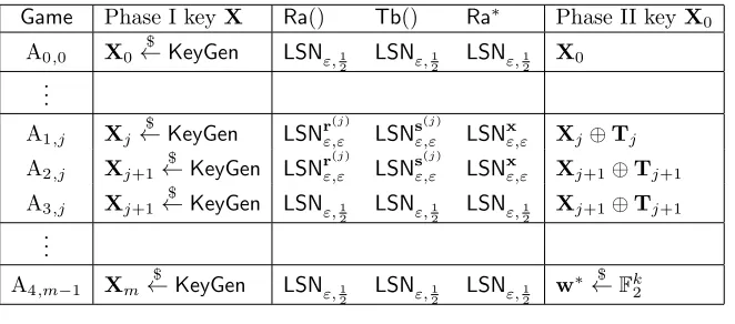
Theorem 19 uses a sequence of games A0,0 (in which the simulator runs theHBNprotocol) through A4,m−1 to show that |AdvHBAN−Adv

A4,m−1

A | ≤2m·εLPN.

Theorem 19. For all efficientAand form=n+ω(logn),k=n−ω(logn),k=ω(logn),

|AdvA0,0

A −Adv

A4,m−1

A | ≤2m·εLPN+ 2k −n

+k2−m= 2m·εLPN+negl

Game Definitions. For almost all games,zi $

←TzX_(·,·,e i),wi

$

←RwX_(·,·,f i),w∗i

$

←Rw∗X0_(·,·,f∗

i) remain the same,

although the random inputs ei,fi,fi∗may vary. The single exception is A4,m−1, in whichw∗ $

←F2 is computed without

the use of any key.

Thus, all the initial games can be completely described by (X,X0,Ra(),Tb(),Ra∗()), the Phase I and II keys and

the sampling algorithms for (a, f),(b, e),(a∗, f∗) respectively. For all games, Figure 6 lists changes between games. x is the secret used by the oracle O = LPNxε that interacts with the simulator. Every game in the sequence generates

s(j),r(j),t(j),Tj in the same way: ∀j∈[m],s(j),t(j) $

←Fn2,r(j)=t(j)⊕x,Tj=Pj_i=0−1r(i)s(i)

> .

Game Phase I keyX Ra() Tb() Ra∗ Phase II keyX0

A0,0 X0 $

←KeyGen LSN_ε,1

2 LSNε,12 LSNε,12 X0 ..

.

A1,j Xj

$

←KeyGen LSNr_ε,ε(j) LSN_ε,εs(j) LSNx_ε,ε Xj⊕Tj

A2,j Xj+1 $

←KeyGen LSNr_ε,ε(j) LSNs_ε,ε(j) LSNx_ε,ε Xj+1⊕Tj+1

A3,j Xj+1 $

←KeyGen LSN_ε,1 2

LSN_ε,1 2

LSN_ε,1 2

Xj+1⊕Tj+1

.. .

A4,m−1 Xm

$

←KeyGen LSN_ε,1 2

LSN_ε,1 2

LSN_ε,1 2

w∗←$ Fk2

Figure 6: Summary of Games

Transitions between games. The proof of Theorem 19 is built from a sequence of games with several types of transitions, which are proven in Corollaries 20–22.

Changing Sampling of b(i),a(i),a∗(i). The first transition type, Corollary 20, hinges upon the computational hardness of LSN(and hence ofLPNby Lemma 17). The transitions between Games A0,0-A1,0 change howb(i),a(i),a∗(i)

are sampled using LSN, and the transitions to and from A3,j change howb(i),a(i) are sampled using LSN. Corollary 20

will follow from the construction of interpolating games.

Switching the key from Xj to Xj+1. In Games A1,j-A2,j, we use Corollary 21 to replace the Phase I and Phase

II keys with nearby keys.

Corollary 21. A1,j andA2,j are equivalent: |Pr[SA1,j]−Pr[SA2,j]|= 0

The proof of Corollary 21 requires Lemma 23, a technical result related toLSN. Lemma 23 uses theLSNdistribution to annihilate the adversary’s contribution s>b0 to w corresponding to rs>. Corollary 21 will then follow from several applications of Lemma 23. This key lemma is actually the raison d’ˆetre ofLSN, although we envision it being useful in other applications as well.

A sufficiently random Phase II key yields w∗ _{indistinguishable from random. For the final step,} Corollary 22 establishes that for sufficiently largem, no adversary can achieve advantage non-negligibly greater than the advantage of the adversary which simply choosesz∗at random.

Corollary 22. |AdvA4,m−1

A −Adv

A3,m−1

A | ≤k2

−m_{+ 2}k−n_{, which is negligible fork < n−ω(logn), m=ω(logn).}

5.2

Interpolating Games: Proof of Corollary 20

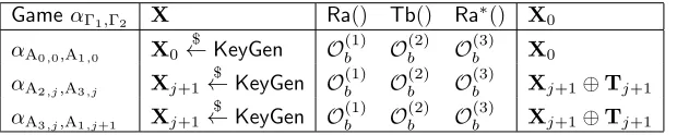
We define interpolating games as shown in Figure 7.

GameαΓ1,Γ2 X Ra() Tb() Ra

∗_{() X}

0

αA0,0,A1,0 X0

$

←KeyGen O_b(1) O(2)_b O(3)_b X0

αA2,j,A3,j Xj+1

$

←KeyGen O_b(1) O(2)_b O(3)_b Xj+1⊕Tj+1

αA3,j,A1,j+1 Xj+1

$

←KeyGen O_b(1) O(2)_b O(3)_b Xj+1⊕Tj+1

Figure 7: Interpolating Games

Proof of Corollary 20. For any adversary A, consider the adversary BO

which constructs game αΓ1,Γ2 from its LSNε,δ

oracle (where δ = 1

2 when b= 0, and δ =ε, otherwise) as follows. B

O

usesO(i)b from Lemma 10 with`= 3. B

O then

constructs a game usingXj $

←KeyGenas both the Phase I and Phase II secret, generatingRa() fromO(1)b andTb() from Ob(2), andRa

∗

fromOb(3). It then runsA, returning 1 ifAis accepted (i.e. |z

∗

⊕w∗| ≤k·u_HBN(ε)), and 0 otherwise. Then

it follows by construction and Lemma 17 that∀(Γ1,Γ2)∈ {(A0,0,A1,0),(A2,j,A3,j),(A3,j,A1,j+1)}and∀A,

|AdvΓ1

A −Adv

Γ2

A|=Adv LSN B

≤εLPN

5.3

Key Switch: the Technical Details

Next, we prove Corollary 21. Corollary 21 is in some sense the core of the security proof: it allows us to change the Phase I and Phase II keys so that they differ by a rank 1 matrix, while the protocol remains indistinguishable from the real protocol. Its proof is based on the following technical lemma.

Lemma 23. Given any(Y0,x,y)∈Fn2×n×F n

2×Fn2,letY1=Y0⊕xy>. For anyb0∈Fn2, and for(a, e)sampled according

toLSNxε,ε, the random variablesW0=. wzY0(a,b0, e)andW1=. wzY1(a,b0, e)induced by(a, e)are identically distributed.

Proof. Define the random variablesGˆawith distributionBerpε,ε

1|ˆa. Recall from Corollary 15 thatGˆadescribes the marginal

wzY1_(a,b0_{, e) =a}>_X 1b

0

⊕e

≡a>X0b0⊕a>xy>b0⊕Ga>_x (13) =a>X0b0⊕

(

G0 ifa

> x= 0

y>b0⊕G1 ifa

> x= 1

≡a>X0b

0

⊕

(

G0 ifa>x= 0

y>b0⊕Ber1 2 ifa

>

x= 1 (14)

≡a>X0b

0

⊕

(

G0 ifa

> x= 0

Ber1 2 ifa

>

x= 1 (15)

≡a>X0b0⊕

(

G0 ifa

> x= 0

G1 ifa>x= 1

(16)

=a>X0b

0

⊕G_a>_x

≡wzY0_(a,b0_{, e)}

Equation 13 follows from conditioning on a>x. Equations 14 and 16 follow from Corollary 16. Equation 15 follows from Fact 2.

Next, we apply the lemma to Phase I and Phase II.

Corollary 24. WhenRa=LSNrε,ε(j),Tb=LSNs (j)

ε,ε,Ra∗=LSNxε,ε, andr(j)=t(j)⊕x, the games constructed from Phase

I and II key pairs(X,Y) and(X⊕r(j)_s(j)>_,Y⊕xs(j)>_{)are indistinguishable.}

Proof of Corollary 24. The proof follows from three applications of Lemma 23: two forRwandTzin Phase I, and one for

Rw∗in Phase II.

RwX(a(i),b0(i),fi)≡wzX(a(i),b

0(i)

,fi)

≡wzX⊕r(j)s(j)

>

(a(i),b0(i),fi) (17)

TzX(a0(i),b(i),ei)≡wzX

>

(b(i),a0(i),ei) ≡wzX>⊕s(j)r(j)

>

(b(i),a0(i),ei) (18)

≡wzX⊕r(j)s(j)

>

(a0(i),b(i),ei) (19)

Rw∗Y(a(i),b0(i),fi)≡wzY(a(i),b

0(i)

,fi)

≡wzY⊕xs(j)

>

(a(i),b0(i),fi) (20)

Equation 17 follows from Lemma 23 applied to (X,r(j)_,s(j)_{). Equation 18 follows from Lemma 23 applied to (X}>

,s(j)_,r(j)_).

Equation 19 follows from the bilinearity ofTz(). Equation 20 follows from Lemma 23 applied to (Y,x,s(j)).

Finally, we need a result that the joint distribution obtained from Equations 17, 19, and 20 is equivalent to the distribution in A2,j.

Corollary 25. With notation as in Figure 6

(Xj+1,Xj+1⊕Tj+1)≡(Xj⊕r(j)s(j)

>

,Xj⊕Tj⊕xs(j)

> )

Corollary 25 will follow from the following technical lemma.

Lemma 26. Let(X1,X2) $

←D, and choose X←$ Un×n independently of (X1,X2). Then the following distributions are

equivalent:

(X⊕X1,X⊕X2)≡(X,X⊕X1⊕X2).

Proof of Lemma 26.

Pr[( ˆX1,Xˆ2) = (X⊕X1,X⊕X2)] = Pr[X=X1⊕Xˆ1∧X=X2⊕Xˆ2)]

= 2−n2Pr[X1⊕Xˆ1=X2⊕Xˆ2] (21)

= 2−n2Pr[X1⊕Xˆ1⊕X2= ˆX2]

= Pr[ ˆX1=X∧Xˆ2=X⊕X1⊕X2] (22)

= Pr[( ˆX1,Xˆ2) = (X,X⊕X1⊕X2)]

Equation 21 and Equation 22 follow from independence ofXfromX1,X2 respectively.

Proof of Corollary 25.

(Xj⊕r(j)s(j)

>

,Xj⊕Tj⊕xs(j)

>

) = (Xj⊕(x⊕t(j))s(j)

>

,Xj⊕Tj⊕xs(j)

>

) (23)

≡(Xj,Xj⊕Tj⊕t(j)s(j)

>

) (24)

= (Xj,Xj⊕Tj+1) (25)

= (Xj+1,Xj+1⊕Tj+1) (26)

Equation 23 follows from the definition of r(j)_{. Equation 24 follows from Lemma 26 applied to D =}n_r(j)_s(j)>_,xs(j)>o_.

Equation 25 follows from the definition ofTj. Equation 26 follows from a simple relabeling.

Proof of Corollary 21. Corollary 21 now follows immediately from Corollary 24 applied to (Xj,Xj⊕Tj) and from Corollary 25.

5.4

A Theorem for Products of Random Matrices

For a randomn×kmatrixA, letSA be the event thatrank(A)< k. For a givenn×kmatrix ˆB(with no zero columns)

and a randomn×mmatrix S, letTBˆ>_S be the event that some row of ˆB>Sis all zero, i.e. ∃isuch thatS>Beˆ (i) =0m. The main result of this section is the following theorem.

Theorem 27. Let A←$ Fn2×k andR,S $

←Fn2×m, for m≥k. Given any Bˆ ∈F n×k

2 such that ∀i∈[k],Beˆ

(i) ₆₌₀n_{, we}

have:

(a) Pr[SA]≤2k−n,Pr[TBˆ>_S]≤k2−m (b) ∀ˆz∈Fk2,Pr[diag(A

>

RS>B) = ˆˆ z|SA, TBˆ>_S] = 2−k

Roughly speaking, Theorem 27 states thatAand ˆB>Sare “degenerate” only with negligible probability, and ifA,Bˆ>S are nondegenerate, thendiag(A>RS>B) is uniformly distributed.ˆ

Proof of Theorem 27(a). First considerSA. We find that

Pr[rank(A)< k] = Pr[∃x∈Fk2\

n

0ko:Ax=0n] (27)

≤ X

x∈_Fk 2\{0k}

Pr[Ax=0n] (28)

= X

x∈Fk2\{0k}

Y

i∈[n]

Pr[(e(i)>A)x= 0] (29)

= (2k−1)· Y i∈[n]

2k−1

2k (30)

≤2k−n

Equation 27 and Equation 30 both follows from rank(M) +rank(ker(M)) =k, for M=A,x respectively. Equation 28 follows from the union bound. Equation 29 follows from independence of the rowse(i)>_AofA.

Pr[∃i∈[k],S>Beˆ (i)=0m]≤ X i∈[k]

Pr[S>Beˆ (i)=0m] (31)

= X

i∈[k]

Y

j∈[m]

Pr[e(j)>SBeˆ (i)= 0] (32)

= X

i∈[k]

Y

j∈[m]

1 2

=k2−m

Equation 31 follows from the union bound. Equation 32 follows from independence of the rowse(j)>_SofS.

We move on to Theorem 27(b). We will need the following two lemmata.

Lemma 28. LetR←$ Fn2×m. Then∀Aˆ ∈F n×k

2 withrank( ˆA) =k≤n,∀Yˆ ∈F k×m 2 , Pr[ ˆA

>

R= ˆY] = 2−km_.

Proof. Each column ˆYe(i) = ˆA>(Re(i)) is an independently random element ofIm( ˆA>). Since ˆAhas full rank, Im( ˆA>) contains all ofFk2, so that each column is a uniformly randomk-bit vector.

Lemma 29. LetY←$ Fk2×m,S $

←Fn2×m. Given anyˆz∈F k

2 andBˆ ∈Fn

×k

2 so that∀i∈[k],S

>_ˆ

Be(i)₆₌₀n_,

Pr[diag(YS>B) = ˆˆ z] = 2−k

Proof. For alli∈[k], lety(i)_=Y>

e(i) _andx(i)_=S>_ˆ

Be(i)_.Then

Pr[diag(YS>B) = ˆˆ z] =

k

Y

i=1

Pr[y(i)>x(i)= ˆzi] (33)

=

k

Y

i=1

n

y(i):y(i)>x(i)= ˆzi

o

|Fn2|

(34)

=

k

Y

i=1

2n−1

2n (35)

= 2−k

Equation 33 follows from expressing the diagonal of the product YS>Bˆ in terms ofY andS>B. Equation 34 followsˆ from independence of they(i). Equation 35 follows from|ker(x(i))|= 2n−1=|Fn2 \ker(x(i))|forx(i)6=0k.

Theorem 27(b) now follows immediately from Lemma 28 and Lemma 29.

5.5

Proof of Corollary 22

We use Theorem 27 to prove Corollary 22, which states that the adversary in A3,m−1cannot do non-negligibly better than

randomly guessing.

Proof Corollary 22. Let R,S be the matrices formed by taking r(j),s(j) as columns respectively: ∀j ∈ [m],Re(j) = r(j)_,Se(j)_=s(j)_{. Then}

m

X

j=1

r(j)s(j)>=

m

X

j=1

(Re(j))(Se(j))>

=R

m

X

j=1

e(j)e(j)> !

S>

=RImS

>

=RS>

AdvA4,m−1 A = Pr              Xm $

←KeyGen(1n), s← A$ T1Xm,RXm(1

n

), ˆ

A←$ Fn2×k,

(z∗,B)ˆ ← A2$ (s,A)ˆ , R,S←$ Fn2×m,

f←$ Bernε,

w∗=diag( ˆA>XmB)ˆ ⊕diag( ˆA>RS>B)ˆ ⊕f

: ∀i∈[k],Beˆ

(i)₆

=0n,

|z∗⊕w∗| ≤k·u_HBN(ε)

             (36)

For any vector ˆz∈Fk2of guesses made by the adversary, it follows from Theorem 27(a) that Pr[SA∨T_Bˆ>_S]≤2k−n+k2−m. It follows from Theorem 27(b) that conditioned onSA∧TBˆ>_S, the distribution ofw∗in A3,m−1 obeys

w∗=diag( ˆA>XmB)ˆ ⊕diag( ˆARS

>_ˆ B)⊕f =diag( ˆA>XmB)ˆ ⊕Berk1

2 ⊕f

=Berk1 2

(37)

Equation 37 follows from Fact 2. SinceBerk1

2 is the distribution ofw

∗

in A4,m−1, Corollary 22 follows immediately

from Equation 37 and Theorem 27(a).

5.6

Soundness and Completeness

We now have all the ingredients required to prove Theorem 19 and Theorem 18, and to determine appropriate parameters to optimize soundness and completeness.

Proof of Theorem 19.

|AdvA0,0

A −Adv

A4,m−1

A | ≤ |Adv

A0,0

A −Adv

A1,0

A |+

m−2

X

i=0

+|AdvA3,i

A −Adv

A1,i+1

A |

+

m−1

X

i=0

|AdvA1,i

A −Adv

A2,i

A |+|Adv

A2,i

A −Adv

A3,i

A |

+|AdvA4,m−1

A −Adv

A3,m−1

A | (38)

≤2m·εLPN+ 2

k−n

+k2−m (39)

Equation 38 follows from the triangle inequality, and Equation 39 follows from Corollaries 20–22.

In A4,m−1, sincew∗ $

←Fk2, for any distribution ofz∗, the distributionz∗⊕w∗is uniformly random. Therefore

Pr[|z∗⊕w∗| ≤k·uHBN(ε)] = Pr[|w ∗

| ≤k·uHBN(ε)]

≤2−k((12−(1+δ))(ε⊕ε)) 2

(40)

Equation 40 follows from the well-known Hoeffding-Chernoff bound, Pr[X ≤(1−µ)·X]≤e−µ2k, forX =Pk i=1Xk

withXi∈[0,1] for alli∈[k]. Recall that withuHBN(ε) = (1 +δ)(ε⊕ε),HBNachieves completenesse−δ 2_k

, i.e. an honest

T fails with probability at moste−δ2k. If we setδ so thatuHBN(ε) = (ε⊕ε)(1 +δ) =1₂(1−δ), we obtain the same bound

ofe−δ2k_{for both soundness and completeness. (ε⊕ε)(1 +δ) =} 1

2(1−δ) results inδ= 1 2−(ε⊕ε) 1 2+(ε⊕ε)

= 1−4ε+4ε2

1+4ε−4ε2. As a result,

we obtain

Pr[|z⊕w| ≤k·uHBN(ε)]≤2 −kδ2

= 2−k

1−4ε+4ε2 1+4ε−4ε2

2

(41)

Proof of Theorem 18.

AdvHBAN≤ |Adv

A4,m−1

A −Adv

A0,0

A |+Adv

A4,m−1

A (42)

≤2k−n+k2−m+ 2m·εLPN+Adv

A4,m−1

A (43)

≤ 2k−n+k2−m+ 2−k

1−4ε+4ε2 1+4ε−4ε2

2!

+ 2m·εLPN (44)

=negl (45)

Equation 42 follows from the triangle inequality. Equation 43 follows from Theorem 19. Equation 44 follows from Equation 41. Equation 45 follows from theLPNassumption and from settingm=ω(logn),k=ω(logn),k=n−ω(logn), andε=θ(1).

6

Conclusion

We have introducedHBN_{, a bilinear version ofHB, and proven its security in theMan-in-the-Middlemodel. Along the way,} we have introduced a new notation the simplifies working with random variables over F2, assembled a useful collection

of lemmas for working with LPN, and introduced the LSNproblem. Additionally, we have designed a new probabilistic verification procedure which is in this case symmetric to the probabilistic prover procedure. We hope that these technical tools will be useful for future work.

We are grateful to Eike Kiltz and David Cash for pointing out a gap in the proof of the version of Corollary 22 in a previous version of this work. We would also like to thank Krzysztof Pietrzak for useful discussions about LPN, and Miaomiao Zhang for helpful remarks on earlier drafts of this work.

References

[AL87] Dana Angluin and Philip D Laird. Learning from Noisy Examples.Machine Learning, 2(4):343–370, 1987.

[BC08] Julien Bringer and Herve Chabanne. Trusted-HB: a low-cost version of HB secure against man-in-the-middle attacks. arXiv, 2008.

[BCD06] Julien Bringer, Herv´e Chabanne, and Emmanuelle Dottax. HB++: a lightweight authentication protocol secure against some attacks. InSecond International Workshop on Security, Privacy and Trust in Pervasive and Ubiquitous Computing (SecPerU 2006), pages 28–33. IEEE Computer Society, 2006.

[DK08] D Duc and Kwangjo Kim. Securing HB against GRS man-in-the-middle attack. caislab.icu.ac.kr, 2008.

[FS09] Dmitry Frumkin and Adi Shamir. Un-Trusted-HB: Security vulnerabilities of Trusted-HB.EPrint, 2009.

[GRS05] Henri Gilbert, Matthew Robshaw, and Herve Sibert. Active attack against HB+_{: a provably secure lightweight}

authentication protocol. Electronics Letters, 2005.

[GRS08a] Henri Gilbert, Matthew Robshaw, and Yannick Seurin. Good variants of HB+ are hard to find. In Proc. Financial Cryptography and Data Security, pages 156–170, 2008.

[GRS08b] Henri Gilbert, Matthew Robshaw, and Yannick Seurin. HB#: Increasing the security and efficiency of HB. In Proc. EUROCRYPT, volume 4965, pages 361–378, 2008.

[HB01] Nicholas Hopper and Manuel Blum. Secure human identification protocols. InProc. ASIACRYPT, 2001.

[JW05] Ari Juels and Stephen Weis. Authenticating pervasive devices with human protocols. InProc. CRYPTO, pages 293–308, 2005.

[Kea93] M. Kearns. Efficient noise-tolerant learning from statistical queries. InProceedings of the 25th ACM Symposium on Theory of Computing, pages 392–401. ACM, 1993.

[KPC+11] Eike Kiltz, Krzystof Pietrzak, David Cash, Abhishek Jain, and Daniele Venturi. Efficient Authentication from Hard Learning Problems. InProc. Eurocrypt, pages 7–26, 2011.

[KSS10] Jonathan Katz, Ji Sun Shin, and Adam Smith. Parallel and concurrent security of the HB and HB+ protocols. Journal of Cryptology, 23(3):402–421, 2010.

[LMM08] X Leng, K Mayes, and K Markantonakis. HB-MP+ protocol: An improvement on the HB-MP protocol. 2008 IEEE International Conference on RFID, 2008.

[OOV08] Khaled Ouafi, Raphael Overbeck, and Serge Vaudenay. On the security of HB# against a man-in-the-middle attack. Proc. ASIACRYPT, 2008.

[Pie10] Krzystof Pietrzak. Subspace LWE, 2010. Manuscript available at _{http://homepages.cwi.nl/~pietrzak/} publications/SLWE.pdf.

A

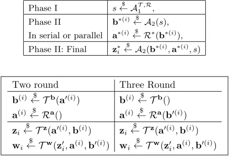
Modeling the Active Security Game

The adversaryAcan be defined as two algorithmsA= (A1,A2). In Phase I,A1 has access to the Phase I oraclesT,R, and outputs its statesfor input toA2.A2submitsb∗(i) _{to the Phase II challengerR}∗

(either in parallel or in serial) and receivesa∗(i)in exchange, as shown in Figure 8. From the model, we see that the reasonHBNcan be used in either two or three rounds is precisely because the computation ofb(i) _{does not depend ona}0(i)_{, anda}(i)_{does not depend onb}0(i)_.

Phase I s← A$ T1,R,

Phase II b∗(i)← A2$ (s), In serial or parallel a∗(i)← R$ ∗

(b∗(i)), Phase II: Final z∗i

$

← A2(b∗(i)_,a∗(i)_{, s)}

Two round Three Round b(i)_{← T}$ b_(a0(i)_{) b}(i)_{← T}$ b₍₎

a(i)_{← R}$ a_{() a}(i)_{← R}$ a_(b0(i)₎

zi

$

← Tz_(a0(i)_,b(i)_{) z}

i

$

← Tz_(a0(i)_,b(i)₎

wi

$

← Tw_(z0

i,a(i),b0(i)) wi

$

← Tw_(z0

i,a(i),b0(i))