A PROJECTIVE APPROACH TO ELECTROMAGNETIC PROPAGATION IN COMPLEX ENVIRONMENTS
E. Di Giampaolo and F. Bardati
Dipartimento di Informatica, Sistemi e Produzione Universita’ di Roma Tor Vergata
via del Politecnico 1, Roma 00133, Italy
Abstract—High frequency methods resort to numerical ray tracing for application to complex environments. A new method based on the geometrical projection performed by a ray-congruence has been developed as a preconditioning of the ray tracing procedure. It builds a visibility tree, i.e., a database, storing information on all possible ray paths inside a scenario. The method gives a solution to a class of open problems of ray tracing techniques: ray missing, double (multiple) counting, termination criterion, calculation upgrade. Other features of the method are the multipath map and the multipath classification that allow the user to know the relevance of multipath at any point of the scenario in advance, before ray-tracing calculation.
The method can be systematically applied to scenarios pertaining to different applications provided that the objects belong to the class of polyhedrons. Reflected and diffracted contributions in a scene are modelled as secondary sources which are handled with an off-line electromagnetic field calculation.
Numerical analysis is provided showing the efficiency of the method.
1. INTRODUCTION
Deterministic models based on Geometrical Optics (GO) and Uniform Theory of Diffraction (UTD) [1] are widely used for high-frequency electromagnetic propagation in large and complex environments such as urban, indoor and terrain scenarios, where multipath prediction is suitable for high bit-rate digital communication. Electromagnetic analysis of automotive, ship, and satellite platforms
also can take advantage of GO/UTD modeling for on-board antenna characterization, coupling, electromagnetic compatibility as well as radar cross section [2–5]. In general, GO/UTD models are advantageous in comparison with other numerical techniques every time constraints on wavelength and scatterer size are satisfied without restriction to a specific application.
Deterministic models require detailed geometrical and morpho-logical information on the propagation environment. Exploiting GO and/or UTD equations, the electromagnetic field is calculated for given positions of source and observer after the ray paths joining the source to the observation point have been determined. Ray-tracing algorithms are used to single out the possible paths between. Ray propagation is affected by multiple interactions with scatterers, so ray tracers are quite laborious requiring a large amount of computational resources. Moreover, they may lose important field contributions and are trou-bled by the handling of complex geometries, the managing of large interaction orders, and the modeling of higher-order diffraction.
A feature common to all ray tracers is that an increased complexity of the propagation environment requires increasing efforts to determine the whole set of possible ray paths. Therefore the ray propagation models, which have been proposed in the literature, are generally designed for the particular scenario that is analyzed. A number of papers has been published on this subject and a comprehensive review is presented in [6]. Both 2-D and 3-D [7–16], ray tracers have been proposed in the case of urban propagation, similarly for indoor propagation [17–21]. Moreover, to overcome the lack of diffuse radiation due to the roughness of the surfaces ray tracing techniques have been recently improved resorting to diffuse scattering models [22] and radiosity [23]. To improve the computational efficiency instead, some of the proposed algorithms exploit geometrical symmetries, such as vertical symmetry for urban environments. Image based models [10– 12] resort to particular visibility algorithms in order to determine visible objects. Another ray-tracing critical feature is the need of a criterion to stop a computation. Indeed, a truncation error occurs when the propagation is stopped at a prefixed interaction order. Recently, a progressive technique [24] has been proposed to counteract the truncation error. Ray missing can be avoided by beam tracers [25– 30] which, however, have other troubles in particular in handling diffraction, which is responsible for communication to shadowed (non-line-of-sight) areas.
the accuracy and reducing the computational effort is not yet fulfilled. To the best of our knowledge, ray missing, termination criterion and calculation upgrade are still open problems that have been marginally faced in literature. Ray missing mainly depends on the ability of visibility algorithms to determine the visible portion of objects and, in particular, the boundary of objects that causes diffraction. A termination criterion is a set of rules that stop computation (i.e., ray-bouncing) along with knowledge of the truncation error. For brevity we call upgrading ability the property of an algorithm to minimize the additional computational effort that is required by the inclusion of further objects in the environment. Usually, a new complete ray tracing is performed when the environment complexity is increased by addition of details. Upgrading techniques, instead, exploit already calculated data as start point for improved calculation. The calculation upgrade has been used in [31] to take the moving of an object into account.
We base our method on a Projective Scheme (PS) which is independent of any particular application and gives a solution to the above mentioned problems improving accuracy without additional computational charge. It avoids ray missing resorting to the concept of ray congruence, which denotes a family of rays that fill up a portion of the three dimensional space including sources and scatterers. Moreover, the truncation error can be estimated by means of the power-density spreading, which is a geometrical parameter independent of the environment morphology. The upgrading techniques exploit a visibility database in conjunction with the projective scheme. The use of a visibility database may resemble the methods in [10–12] and [29] which also make use of it. While the methods in [10–12] are aimed at determining the visibility of objects in order to accelerate ray tracing computation, our method determines the portion of three dimensional space that is filled with a ray congruence, i.e., a frustum. Once the frustum is obtained no further ray-intersection test is necessary because the rays through a point are found enforcing a belonging test. Our method also overcomes the ambiguity errors typical of beam tracers [29], i.e., a ray contribution shared by adjacent beams may be omitted or counted twice. Including all possible ray-paths, the projective scheme permits to determine any multipath contributions at any point of the scene without making ray-tracing calculation. It allows the user to single out regions of the scene affected by a specific multipath and to restrict the extensive ray-tracing procedure to them.
surface and impinge on some scatterers. Any ray of the bundle is a projection line and the ray congruence that a ray belongs to defines the kind of projection (e.g., stigmatic, astigmatic). According to the above definition, the reverse rays project the objects (3D) on which the rays impinge onto the surface (2D) from where they start. If a bundle starts from a caustic (e.g., a point or a line), the surface of the corresponding wave-front is used for projection. As a result of the projection, the portions of the scatterers impinged by the ray bundle are mapped onto a subset of the start surface. Due to the property of the projective operator to be continuous, the mapping preserves the environment topology [33]. Topological relationships such as adjacency and belonging are useful to counteract the ambiguity error and to reduce the size of the visibility database.
An n-order ray congruence (n denote the interaction order) is generated by diffraction or reflection or transmission at a geometric element (e.g., a line or a surface) belonging to an object in the scenario that has been lighted by an impinging radiation of order n−1. An edge-diffracted ray congruence is modeled by Keller’s law, while a reflected or transmitted ray congruence is modeled by Snell’s law. The projective scheme makes pairs of visible points passing from the (n−1)th to the nth interaction. A ray path is determined by a chain of visible pairs when the interaction order is ranged to an orderN.
Arrangement of visibility chains is a complicated matter in the case of complex environment, therefore we have developed an iterative procedure which borrows methods and data structures from Computer Graphics [34]. It collects and stores the visibility information between geometrical elements in a visibility database preserving the hierarchy induced by the interaction order n. The visibility database has the structure of a tree, whose root is the primary source. The data related to the geometrical elements that are visible by the source are stored in first-order (n = 1) nodes, while the data pertaining to the elements that are visible through the rays from first-order nodes are stored in second-order nodes, and so on according to the projective scheme. The procedure is completed when an a-priori number of interactions has been reached or the power-density spreading is lower than a given threshold. The algorithm falls in the class of iterative methods since it attempts to model electromagnetic propagation in complex environments by finding successive approximations to the field problem.
exploring the visibility tree, while the second step performs the field calculation.
We shall consider scenarios whose objects are polyhedrons with flat and convex facets and straight edges. Even if some scenarios may be oversimplified using the objects of this class, polyhedrons are frequently used in a large number of applications. No further restriction to particular symmetry, shape or application has been introduced. Three kinds of interaction can be envisaged with polyhedrons, i.e., reflection and transmission at facets, diffraction at edges and corner diffraction. Unlike the other interactions, corner diffraction is not explicitly treated in this paper as it is modeled like a stigmatic point source that is described in depth. The space among the objects is filled by a dielectrically homogeneous medium, e.g., a vacuum.
A numerical code implementing the projective scheme has been developed. In order to show its advantages and the computational charge three examples of applications are discussed. Two simple scenes with few objects are used to assess the accuracy of the electromagnetic calculation. The third example refers to a typical urban scenario and is used to test both the reliability and the computational charge.
The paper is organized as follows. The next section will introduce the projection scheme. In Section 3, the algorithm organization will be illustrated, while its main features together with solutions to the termination and upgrading problems will be discussed in Section 4. Results of the numerical analysis will be presented in Section 5. The ray-congruence equations together with details in handling the ray missing problem are summarized in the appendix.
2. THE PROJECTIVE SCHEME
We consider an environment of objects and wavefront-radiating sources. Wavefronts and objects are modeled with an arrangement of polygonal facets. A ray-congruence starts from the surface of objects or wavefronts and impinges on the surfaces of other objects. At the nth iteration, ray-congruences of order (n−1) impinge on the surfaces of some objects after leaving their start surface Sin−1. A 0-order congruence starts from a wavefront of a primary source.
Consider the ith congruence of order n−1, Mni−1, whose rays have origin atSni−1 and end atsni−1. Sni−1 is known from the previous computational step, while sin−1 has to be determined. The points of si
n−1 can be projected onto points of Sni−1 using the rays ofMni−1 as
from the set {Σp} of all the facets by means of the projection of each facet Σp onto Sni−1 and determining the visible portion ωp of Σp, i.e., si
n−1 =
p ωp
. The elements of {Σp} are ordered according to their
distance fromSni−1. When the (p+ 1)th facet is projected onto Sni−1, the corresponding ray bundle can be partially or totally obstructed by the facets from 1 to p, that have been already projected. In other words, the projection Ωp+1 of Σp+1 is a portion of the starting surface
Si
n−1 deprived of the areas that are in visibility with closer facets, i.e.,
Ωp+1 ⊂Sni−1−Cp, (1) where
Cp = p
q=1
Ωq (2)
if Ωp+1 is empty, then Mni−1 cannot make Σp+1 visible by Sni−1.
Ap = Sni−1 −Cp is the available area for projection onto Sni−1
of the facets that are more distant than Σp, while Cp denotes the complementary of Ap, i.e., Ap ∪Cp = Sni−1. If Ap is empty no other facet is visible by means of Mni−1. Between ωp and Ωp there is a one to one correspondence being one the projection of the other by means of a ray bundlemp, subset ofMi
n−1.
It is worth observing that the space si
n−1 that is visible by Sni−1
throughMni−1, is dynamically obtained when the counterpis increased from 1 to the number of facets.
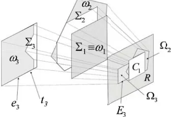
An example of the projective scheme is given in Fig. 1 for a ray congruence from a rectangle R as the start surface Sni−1, and three
facets Σp,(p= 1,2,3) ordered according to their distance fromSi n−1.
The ray congruence is stigmatic from a point source not shown in the figure while R is a facet in the wavefront polyhedral approximation. The visible portions (ωi, i= 1,2,3) of Σ1, Σ2 and Σ3 are shadowed.
Σ1 is fully visible with footprint Ω1 coincident withC1. The visibility
of Σ2 is tested in A1 =R−C1, and so on.
The boundary Γp of Σp deserves particular attention when it is projected by Mni−1. Let tp denote a side of Γp, i.e., a segment of straight line since Γp is a polygonal contour. After projection, tp will be mapped onto a segmentTpofSin−1. However, only the portionEpof Tp that belongs toSin−1−Cp is connected by non obstructed rays to a segmentep⊆tp, whereCpis obtained by Equation (2). In this case, ep is an element of the visible spacesin−1. Iftp is not a boundary between coplanar facets, thenep is a diffracting edge. IfEp,ep are empty sets, no piece of tp is source of diffracting rays. The construction will be repeated for all the sides of Γp and for all p in order to determine the whole set of visible edges {ep}in−1 that diffract the ray congruence Mi
n−1.
In the last step of the nth iteration, sin−1 is stored as a next-order start surface, Sni. Sni is the set of the start points of the new ray congruence, Mni, obtained by reflection or transmission of Mni−1. In addition, each element of {ep}in−1 is source of a diffracted ray congruence. We model a diffracted wavefront from the kth edge as a polyhedral surface,Snk[35]. The rays of Mnk start from the points of Sk
n.
In conclusion to the current iteration, we are left with a set of start surfaces and related ray congruences. Some of them approximate the contours of scatterers and are referred to as material surfaces, while the remaining surfaces that model diffracted wavefronts are purely geometrical. In the next iteration, each one will be propagated to the environment according to the above procedure.
3. ALGORITHM ORGANIZATION
Planar, spherical and cylindrical ray-congruences model primary sources, while astigmatic ray-congruences model wedge diffraction (Appendix B). With the exception of planar ray-congruence, all the others start from caustics, while their wavefronts are curved surfaces that are approximated to polyhedrons in the projective scheme. Wavefronts are approximated preserving the one-to-one correspondence between rays and points of the surface.
The six faces of a cube are used to approximate the spherical wavefront starting from a stigmatic caustic (Fig. 2). Six pyramidal solidsWi, i= 1, . . . ,6 are associated with the faces of the cube. Each Wi has vertex at the caustic point and square cross-section. Theith face is the start-surfaceS0i of theith ray-congruenceM0i. The portion of the pyramidWi lying beyond S0i is used by the visibility test.
An astigmatic ray-congruence has a square cylinder as geometrical surface. The cylinder has the axis coincident with the axial caustic. Since an astigmatic raycongruence is bounded in the axial direction by two cones, i.e., the Keller’s cones with vertices at the axial-caustic end-points, the cylinder portions beyond the cone/cylinder intersections are cut away. With reference to the cylinder faces, the contour of each face has two straight edges parallel to the axis and two curved edges which are the intersection of the planes for the faces with the cones as shown in Fig. 3. The curved edges are arcs of parabolas that are approximated to polygonal lines. When an astigmatic ray-congruence starts from a wedge by diffraction, the angular sector interior to the wedge is cut out from the cylindrical surface. At the most, four adjacent start-surfaces Si
n−1, i = 1, . . . , 4 are used for projection. The ith volume Wi is a
polyhedron having Sni−1 as cross-section and wedges that converge to either of the caustic end-points. The portion ofWi lying beyondSni−1 is used by the visibility test.
VolumeWi is also said view-volume [32], it is a 3D solid extending to ∞ and filled by a ray-congruence. Its basis is a start surface, e.g., Si
n−1. View-volume shape and size depend on the ray-congruence
Mi
n−1 and the shape of Sni−1. To speed up computations, we use
Wi
Si 0
Figure 2. A wavefront from a stigmatic source approximated to a cube. View-volume Wi corresponding to faceS0i (dashed) also shown.
Wi cu
cd a b
Figure 3. A wavefront from an astigmatic source approximated to four surfaces Sin−1, i = 1, . . . , 4. View-volume Wi and axial caustic having end-points a, b also shown. cu and cd are Keller’s cones bounding the view-volume.
At step n, the algorithm projects the elements of {Σp}i
n−1 onto
Si
n−1. Operatively, each facet Σp is projected onto αq, i.e., onto the plane to whichSi
n−1 belongs. Due to Σp convexity, only the polygonal contour Γp is projected. The projection of a pointQ∈Γp is found as the intersection between αq and the straight-line rQ passing through Q and belonging to the ray-congruence Mni−1. The equation for rQ depends on two parameters that are found by the equations given in Appendix B, in accordance with the type of ray-congruence. Since both plane and spherical ray-congruences project straight lines into straight lines, the shape of Γp is preserved after projection, therefore, only the vertices of Γp are projected. In general, however, an astigmatic ray congruence projects a straight line, e.g., a side of the contour, into a curve (Fig. B2), because different projecting lines generally belong to distinct Keller’s cones. Computationally, such a curved projection is approximated by a polygonal line having vertices at the projections on αq of suitably sampled points of Γp. The set of rays passing through the boundary of the visible portion ωp ⊂ Σp, i.e., ∂ωp, delimits the portion of the ray-congruence that is impinging onωp.
4. ALGORITHM MAIN FEATURES
4.1. Visibility and Ray Missing
The operations on the ith ray-congruence at iteration n of the projective scheme are organized as follows. First the subset{Σp}in−1 of the h facets that are completely or partially included inside the view-volume is determined, then these facets are sorted according to distance from Sin−1 and projected starting from the nearest surface, and finally secondary sources (i.e., visible surfacessin−1 and diffracting edges{ep}in−1) are determined and stored in the tree database as new branches preserving the parent-child relationship. The iteration arrives to an end when either condition holds: (i)Sni−1−Cp =∅ for some p, i.e., the whole start surface has been mapped onto visible facets/edges; (ii) all the facets of {Σp}in−1 have been projected. In the last case, m∞ = Mni−1 − h
p=1
mp is the ray-bundle that does not impinge any
facet while it propagates undisturbed to∞.
is lower than a given threshold as is exposed in Subsection 4.2. Since the algorithm routinely explores the whole{Σp}, no object in the scenario is excluded from the visibility test, therefore it prevents any loss of contribution or twice-counting error from any visible point. This feature is illustrated in Appendix A.
4.2. Termination Criterion
The procedure is stopped when the order n of iteration exceeds a threshold. Alternatively the iteration is stopped when the power density radiated by secondary sources is lower than a threshold. As the algorithm postpones field-strength calculations to a stage that follows projections, we introduce a criterion based on radiated-power spreading factor to determine if that threshold is exceeded.
A source projecting the visible surface ωp ⊂ Σp onto its image Ωp⊂Sni−1, spreads power with a factor
spp≤ area
(Ωp)
area (ωp)nˆS·nˆp, (3) where ˆnS and ˆnp are unit vectors orthogonal to Sni−1 and Σp, respectively. Consider now an ordered sequence ofN ray-congruences Mi
n, n = 0, . . . , N − 1, related to each other by parent-child relationships. The cumulative spreading factor of the sequence is
spN = K N−1
n=1
spn, where K takes into account the primary source
which corresponds to n = 0, and K = s−2 or K = s−1 in the case of a stigmatic source or an astigmatic one, respectively. Heres is the minimum distance between the caustic and the start-surfaceSi
0. When
spN < spT (4)
with spT a threshold, MNi−1 contributes to the field at a point P for less than an equivalent source located in the line-of-sight withP at a distanceRP from it. RP =spT−1/2 if the primary source is astigmatic, while RP = spT if it is stigmatic. Condition (4) is normally used to stop the iterations along each ray bundle from a primary source. It should be noted that, since a planar ray-congruence is still planar after reflection from a flat facet, the cumulative spreading factor is unitary during projective iterations so that the termination criterion has no effect in stopping reflections. A criterion based on the maximum number of iterations is therefore used in such a case.
large that few iterations are normally sufficient to have the spreading factor less than a threshold. On the contrary, a larger number of iterations is often necessary to obtain the desired spreading factor in regions with more objects. For these reasons the stopping criterion based on the spreading factor, if compared to the criterion based on the maximum interaction order, has the advantage of reducing the number of secondary ray-congruences and iterations in some regions of the scenario shortening the computational time and reducing the size of the visibility-tree.
4.3. Calculation Upgrade
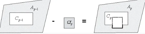
To show this feature we consider the simple environment depicted in Fig. 1, where the ray congruence starting from a rectangle,R, projects the visible portions ωi of Σ1, Σ2 and Σ3 into Ωi, (i = 1,2,3). The visibility tree consists of a root node storing the ray congruence through R, three child-nodes storing the reflected ray congruence and several more nodes storing diffracted ray congruences. If a new object, Σ4,
is included in the environment (Fig. 4) the new visibility tree can be obtained without making a new calculation. The previously calculated visibility tree can be augmented by addition of a sub-tree that take into account shadowing, reflection and diffraction by Σ4. The shadowing
by Σ4 is also a frustum, which intersects the objects placed behind
Σ4 (Fig. 4). The projection of that shadow partially obscures the
reflected and diffracted ray congruences from Σ1 and Σ2 as well as
higher order ray congruences. To take this shadowing into account the existing visibility tree should be modified by subtracting the shadowing frustum from all the obscured ray congruences. As an alternative, the computation of shadowing can be postponed to the procedure for ray-path determination (Subsection 4.4).
The use of upgraded visibility trees is particularly useful for
Figure 4. The scene of Fig. 1 is enhanced with facet Σ4. The
environments with moving and standing objects. A preliminary calculation determines the static visibility tree neglecting the moving objects, then the sub-tree of a moving object is appended to the static tree in order to perform field calculation and then is removed. As this kind of scenarios are time variant, the time domain analysis is performed by means of a sequence of snapshots of the scene. For each snapshot only the sub-trees of moving objects are calculated. This procedure has been used in [31] for the electromagnetic characterization of inter-vehicle communications.
4.4. Field Analysis
The tree-database calculation is performed only once for a given scenario and source position while the field can be calculated at any point of the 3D space exploiting information stored into the database. Field calculation is under the user control and can be repeated any time changing the observation point as well as parameters concerning the morphology of the scenario and antennas.
Including all possible ray-paths, the visibility tree permits to determine any multipath contributions at any point of the scene without making extensive ray-tracing calculation. For a given sub-domain of the scene (e.g., a plane) the user can visualize all ray-congruences passing through it. If the sub-domain is a plane, a map of the multipath is obtained as superposition of the footprints (i.e., the cross-sections) of the ray-congruences passing through the plane. Consequently, if the user is searching the field due to particular multipath contributions, he can exploit this map to single out the regions of the sub-domain affected by that particular multipath. The ray-tracing procedure can be restricted to these regions neglecting the others. Moreover, a classification of the strength of multipaths can be made on the basis of the cumulative spreading factor. These features permit to speed up the analysis of multipath in large and complex scenes like an airport [39].
To determine the field at a pointP inside the scenario a two-step procedure is used. First the ray-paths from a primary source to P are determined by exploiting the data stored in the visibility tree, then the field is calculated along all ray-paths, the total field at P resulting as their vector sum.
This is the only test to determine whether a specific ray is passing through a point. To determine the folded ray path between each node and the primary source, we explore the visibility tree from that node to the root by following a path through the branches, with no jumps. Doing this, an ordered sequence of start-surfaces Sni (or ray-bundles Mi
n) is determined starting fromSmi −1, P. Each ray path is a polygonal line in 3D-space, with vertices at Pni ∈Sni, when the interaction level n ranges from 0 to m. From a computational point of view, the vertices are determined starting from P, with sequential projections using Equations (B1)–(B3) and (B5) in accordance with the type of ray-congruence.
Field calculation is performed applying GO/UTD equations to the folded ray path. While the geometrical information useful to electromagnetic field computation (e.g., path length, curvature radius, spreading factor) is gathered during ray-path calculation, data on the primary-source radiation properties, as well as operation frequency and material properties of objects can be arbitrarily inserted by the user. This step can be repeated any time.
5. NUMERICAL ANALYSIS
A numerical code implementing the algorithm has been developed. In order to show the usefulness of the projective approach and its computational charge three examples of application are discussed. Two simple scenarios with few objects are used to assess the accuracy of the electromagnetic calculation. They were previously used in [40] and [41], where both measurements and simulated data are reported. As a third example a typical urban scenario [42] is analyzed to test both the reliability of calculations and the computational charge. Since computational requirements as well as visibility-tree size increase with the scenario’s complexity and the number of interactions, an urban scenario represents a good test bed. In each example the primary source is a spherical ray congruence with the radiation pattern of the antenna used in the measurement.
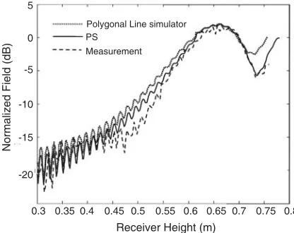
In order to evaluate the effects of many reflected and diffracted contributions, the first scenario consists of a scaled model of urban environment including three perfect-electric-conductor (PEC) objects [40], a transmitter and a receiver. Fig. 5 shows the geometry together with the ray-paths contributing to the field at the receiver point.
(m)
Rx
Tx 0.7
0.6
0.5
0.4
0.3
0.2
0.1
0
(m) 2
0 -2
-0.5 0 0.5 1 1.5 2 2.5 3
(m)
Figure 5. A scaled model of three buildings with PEC walls on a ground. Ray paths to an observation point on a vertical line also shown (dashed lines).
5
0
-10
-15
-20 -5
Normalized Field (dB)
Receiver Height (m)
0.3 0.35 0.4 0.45 0.5 0.55 0.6 0.65 0.7 0.75 0.8
Polygonal Line simulator PS
Measurement
Figure 6. Comparison between PS algorithm and published results for the scene in Fig. 5. Hard-polarization of electric field is shown.
published data.
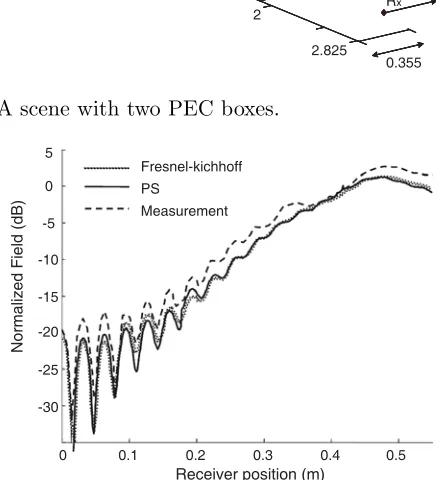
The second example consists of two PEC boxes (Fig. 7). It is a full 3D model [41] where both measurements and simulations have been performed without exploiting symmetry. The field is sampled at points of a line placed behind the boxes and partially in line-of-sight with the transmitting antenna. Diagrams in Fig. 8 compare our calculation with measurements and the Fresnel-Kirchhoff method used in [41]. A high degree of correspondence with published measurements and diagrams has been achieved.
Being three-dimensional UTD-based, the proposed method has the advantage to be computationally easier than the Fresnel-Kirchhoff integral method which belongs to the class of integral equation based methods and more effective than the PL method which, being
two-0.1352 (m)
0
0.5 (m) 1
1.5 2
2.825
0.355 Rx Tx
Figure 7. A scene with two PEC boxes.
Fresnel-kichhoff PS
Measurement
Normalized Field (dB)
5
0
-5
-10
-15
-20
-25
-30
Receiver position (m)
0 0.1 0.2 0.3 0.4 0.5
a
(m)
500 600
400
300
(m) 200
100
0 1000 800 600 400 200 0
source
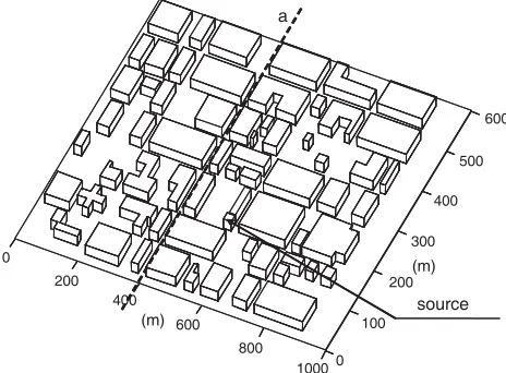
Figure 9. A model of urban environment.
dimensional UTD-based, neglects reflected and diffracted contributions outside the plane where it is working.
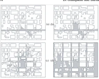
The urban scenario shown in Fig. 9 consists of 64 buildings with 432 facets, 910 edges and ground. Ground and buildings are dielectrically homogeneous with relative permittivity εr = 7 and conductivity σ = 0.2 (S/m) while the height of each building is higher than the source position. The source is a half-wavelength dipole at 910 MHz located at 8.5 m from ground as shown in Fig. 9, where the dashed line labeled (a) shows the points where the electromagnetic field has been calculated. Field points are at 3.65 m above the ground in the middle of the street. The distance between two consecutive points is 1 m.
(a) (b)
(c) (d)
Figure 10. Multipath maps (grey areas) of direct (a), 1st-order reflected (b), 10th-order reflected (c) and 1st-order diffracted, (d) contributions.
measurement PS
Path Loss (dB)
70
80
90
100
110
120
(m)
0 100 200 300 400 500 600
Fig. 11 together with published measurements [42]. In spite of the incomplete knowledge of the scenario’s characteristics which has been reconstructed starting from the topographic map shown in [42], the agreement with published diagrams is fair. To test the computational charge reflections are calculated up to the tenth order while only first order diffraction is considered. The overall computational time is just over 100 s. The time for storing the visibility tree is about 100 seconds while few seconds are necessary for field calculation at 600 points of line (a). Also few seconds are necessary to visualize a multipath map. The computational time is a fraction of second for the two other scenarios. Computations have been performed with a portable PC Pentium Mobile at 2.0 GHz and 512 MB of RAM).
6. CONCLUSION
The proposed PS tracer exploits geometrical tools for GO/UTD field computation in complex environments with polyhedral objects. Direct transmission, reflection and edge diffraction are included in the tracer. The visibility test between any two elements in the scenario is performed according to a projective scheme that makes the tracer free from missing or ambiguity errors. Ray-paths between a source and observation points are calculated exploring the database. While the visibility database is calculated only once for a given scenario and primary source, field computation can be repeated with less computational cost changing observation points and parameters such as frequency and materials. The results of the numerical analysis show that the tracer is accurate and fast. The projective scheme here has been proposed in the frame of a backward tracer marching from observation points to primary sources. A forward ray-tracer where rays are shot and bounced can also take advantage of the projection method, because the ray density from secondary sources can be arbitrarily fixed by a solver thus avoiding both aliasing and receiving sphere problems that are typical of most existing forward ray-tracers.
APPENDIX A. RAY MISSING AND AMBIGUITY ERROR
In some beam tracers the decision whether an individual ray belongs to either adjacent beams is a source of error since a contribution may be omitted or counted twice. In this subsection we show that PS algorithm does not have these drawbacks.
Assuming that each Σp is a planar convex polygon we denote its footprint by Ωp in the absence of obstructions by closer objects. Since the projection operator is continuous, a line segment u ⊂ Σp connecting any pair of points of Σp, has a unique imageU ⊂Ωp after projection. The intersectionU∩Ap−1, if non-empty, belongs to Ωpand is the projection of the visible portion ofu. We assume that whether a point lies in the interior of a given region can be numerically assessed without error. The projective scheme therefore prevents any loss of contribution or twice-counting error from any visible internal point.
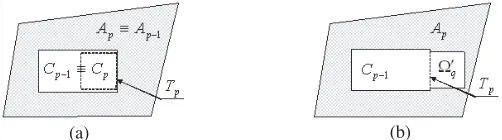
It is not yet excluded, however, that these errors can be localized at the boundaries. To discuss this case, lettp be a side of the contour that is projected ontoTp. EvidentlyTp belongs to the boundary of Ωp. It is easily verified that, for p >1, tp is visible if, in addition, Tp is a side of the boundary of Ap =Ap−1−Ωp. Alternatively, the following criterion can be adopted, which is preferable from a computational point-of-view:
if Tp ⊂Ap−1 thentp is visible (A1) In Fig. A1, first a partition ofSni−1 intoAp−1 andCp−1 is shown. The
two areas are shadowed and clear, respectively. Then Ωp is subtracted to produce a new partition of Sni−1 into Ap and Cp. The Ωp contour is split into two parts that lie inside Ap−1 (bold line) and Cp (dashed
line), respectively. They are the visible and non-visible parts of the contour, in that order. Enforcing test (A1) onTp avoids the missing of a possible contribution bytp. Test (A1) is repeated for all the sides of Σp. It is based on the assumption thatAp−1 is an open set, i.e., it does
not contain its boundary. However, to prevent any ambiguity owing to
(a) (b)
Figure A2. A boundary Tp shared by two facets. The facet closer to the ray start-surface already recognized as visible.
numerical computation, if test (A1) is not fulfilled the following further test can be enforced:
if Tp ⊂Cp thentp is non-visible (A2)
To discuss the missing and twice-counting errors, we observe that a side tp can be shared by two adjacent facets, Σp and Σq, belonging to the same material surface, so that Tp and Tq coincide on a linear segment U. In another case, Σp and Σq are not adjacent since they belong to different material surfaces, but the projections Tp and Tq coincide on U. Assume p > q, i.e., Σq is closer to Sni−1 than Σp, so that tq has already been recognized as visible. A properly designed procedure has to recognize tp as non-visible. Two cases are possible, according to whetherCp−1and Ωp lie on the same side with respect to
Tp or not, as shown in Fig. A2(a) and Fig. A2(b), respectively. In both cases test (A1) is not passed becauseTp does not lie in the interior of Ap−1, while test (A2) is passed, confirming tp as non-visible.
APPENDIX B. RAY CONGRUENCE EQUATION
In any ray-congruence radiated by a source, each ray is determined by the point the ray has in common with a reference surface S, i.e., a wavefront, where the initial conditions: ray-direction, wave amplitude and eikonal are given.
The ray-congruence equation depends on two parameters specifying such a point. S is a plane for a plane wave congruence. In a local Cartesian frame with the z-axis normal to S, the ray for a point Q≡(x, y, z) has the general equation
r(t) =uxˆ+vyˆ+tˆz u =Q·xˆ
v =Q·yˆ
where the projectionsu,vlabel the ray andtis the distance ofQfrom S. ˆx, ˆy,zˆare unit vectors parallel to the axes. Underlining is used here to distinguish between a geometrical point,Q, and its representation, Q, as the vector pointingQfrom the origin.
In spherical coordinatest, θ, φ, the spherical ray-congruence with origin at a point r0 has the equation
r(t) =tˆs(θ, φ)
with ˆs(θ, φ) = ˆxsinθcosφ+ ˆysinθsinφ+ ˆzcosθandtthe distance of r from r0. The ray for a pointQis labeled byθ, φ that are given by
θ = arccos
−Q ·zˆ
Q (B2)
φ = ⎧ ⎨ ⎩
γ (ˆz׈x)·Q≥0
2π−γ if (ˆz׈x)·Q <0
0 γ = 0 or 2π
(B3)
where
γ= arccos
Q·xˆ Q−
Q·zˆzˆ
Wedge diffraction originates an astigmatic ray congruence starting from the edge. Any wedge-diffracted ray-congruence is described, exactly or approximately, by two linear caustics [35]. The first caustic is a focal line coincident with the edge and is referred to as axial caustic, while the second caustic is an arc of circle with center,O, on the edge and lying on a plane orthogonal to the edge (Fig. B1). Since the Keller’s law links the diffraction-cone angle to the diffracting point D, the two parameters labeling an astigmatic ray congruence are an abscissawalong the edge and an angleφaround the edge. Considering the edge oriented along thez-axis of a Cartesian reference frame with origin atO, a ray from Dis the straight line.
r(t) =D+tˆs(w, φ)
with
ˆ
s(w, φ) = R
cosφxˆ+ sinφyˆ+wzˆ
√
R2+w2 (B4)
w w
r
cu
E
cd
D
O
φ Γ
R
Figure B1. Ray r diffracted at D. Edge E (vertical line) and circle are caustics. cu and cd Keller’s cones bounding the astigmatic ray-congruence.
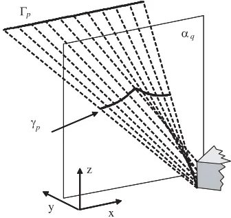
Γp
q
p
α
γ
z
y
x
Figure B2. Wedge diffraction: astigmatic projection (curveγp) of a straight line Γp onto a plane αq. Projecting rays (dashed line) also shown.
A ray passing through a pointQ has parameters
w= R
R+Q−Q·zˆzˆ
Q·zˆ (B5)
while φis given by (B3).
by the Keller’s cones at the edge end-points.
ForR→ ∞ we obtain a cylindrical wave withw= (Q·zˆ).
REFERENCES
1. Kouyoumjian, R. F. and P. H. Pathak, “A uniform theory of diffraction for an edge in a perfectly conducting surface,”
Proc. IEEE, Vol. 62, 1448–1461, November 1974.
2. Hussar, P., V. Oliker, H. L. Riggins, E. M. Smith-Rowland, W. M. Klocko, and L. Prussner, “AAPG2000: An implementation of the UTD on facetized CAD platform models,”Ant. Prop. Mag., Vol. 42, No. 2, 100–106, 2000.
3. Wang, N., Y. Zhang, and C.-H. Liang, “Creeping ray-tracing algorithm of UTD method based on NURBS models with the source on surface,” Journal of Electromagnetic Waves and
Applications, Vol. 20, No. 14, 1981–1990, 2006.
4. Jin, K.-S., T.-I. Suh, S.-H. Suk, B.-C. Kim, and H.-T. Kim, “Fast ray tracing using a space-division algorithm for RCS prediction,”
Journal of Electromagnetic Waves and Applications, Vol. 20,
No. 1, 119–126, 2006.
5. Bang, J.-K., B. C. Kim, S.-H. Suk, K.-S. Jin, and H.-T. Kim, “Time consumption reduction of ray tracing for RCS prediction using efficient grid division and space division algorithms,”
Journal of Electromagnetic Waves and Applications, Vol. 21,
No. 6, 829–840, 2007.
6. Iskander, M. F. and Z. Yun, “Propagation prediction models for wireless communications systems,” IEEE Trans. Microwave
Theory and Technique, Vol. 50, 662–673, March 2002.
7. Yun, Z., Z. Zhang, and M. F. Iskander, “A ray-tracing method based on the triangular grid approach and application to propagation prediction in urban environments,” IEEE
Trans. Antennas Propag., Vol. 50, 750–758, May 2002.
8. Rizk, K., J. F. Wagen, and F. Gardiol., “Two-dimensional ray-tracing modeling for propagation prediction in microcellular environments,”IEEE Trans. Veh. Technol., Vol. 46, 508–517, May 1997.
9. Liang, G. and H. L. Bertoni, “A new approach to 3-D ray-tracing for propagation prediction in cities,” IEEE Trans. Antennas
Propag., Vol. 46, 853–863, June 1998.
and microcell scenarios,” IEEE Antennas Propag. Mag., Vol. 40, 15–27, April 1998.
11. Torres, R. P., L. Valle, M. Domingo, and S. Loredo, “An efficient ray tracing method for radiopropagation based on the modified BSP algorithm,” IEEE Veh. Technol. Conference, Vol. 4, 1967– 1971, September 1999.
12. Ng, K. H., E. K. Tameh, A. Doufexi, M. Hunukumbure, and A. R. Nix, “Efficient multielement ray tracing with site-specific comparisons using measured MIMO channel data,”IEEE
Trans. Veh. Technol., Vol. 56, 1019–1032, May 2007.
13. F¨ugen, T., J. Maurer, T. Kayser, and W. Wiesbeck, “Capability of 3-D ray tracing for defining parameter sets for the specification of future mobile communications systems,” IEEE Trans. Antennas
Propag., Vol. 54, 3125–3137, November 2006.
14. Chiu, C.-C. and T.-C. Tu, “Path loss reduction in an urban area by genetic algorithms,” Journal of Electromagnetic Waves and
Applications, Vol. 20, No. 3, 319–330, 2006.
15. Liang, C.-H., Z.-L. Liu, and H. Di, “Study on the blockage of electromagnetic rays analytically,” Progress In Electromagnetics
Research B, Vol. 1, 253–268, 2008.
16. Kara, A. and E. Yazgan, “Modelling of shadowing loss due to huge non-polygonal structures in urban radio propagation,”Progress In
Electromagnetics Research B, Vol. 6, 123–134, 2008.
17. Yang, C.-F., B.-C. Wu, and C.-J. Ko, “A ray tracing method for modeling indoor wave propagation and penetration,” IEEE
Trans. Antennas Propag., Vol. 46, 907–919, June 1998.
18. Suzuki, H. and A. S. Mohan, “Measurement and prediction of high spatial resolution indoor radio channel characteristic map,”
IEEE Trans. Veh. Technol., Vol. 49, 1321–1333, July 2000.
19. Teh, C. H. and H.-T. Chuah, “A path-corrected wall model for ray-tracing propagation modeling,”Journal of Electromagnetic Waves
and Applications, Vol. 20, No. 2, 207–214, 2006.
20. Chen, C.-H., C. L. Liu, C. C. Chiu, and T. M. Hu, “Ultra-wide band channel calculation by SBR/IMAGE techniques for indoor communication,” Journal of Electromagnetic Waves and
Applications, Vol. 20, No. 1, 41–51, 2006.
21. Liu, Y.-J., Y.-R. Zhang, and W. Cao, “A novel approach to the refraction propagation characteristics of UWB signal waveforms,”
Journal of Electromagnetic Waves and Applications, Vol. 21,
No. 14, 1939–1950, 2007.
“Measurement and modelling of scattering from buildings,”IEEE
Trans. Antennas Propag., Vol. 55, 143–153, January 2007.
23. Kloch, C., G. Liang, J. B. Andersen, G. F. Pedersen, and H. L. Bertoni, “Comparison of measured and predicted time dispersion and direction of arrival for multipath in a small cell environment,” IEEE Trans. Antennas Propag., Vol. 49, 1254– 1263, September 2001.
24. Chen, Z., H. L. Bertoni, and A. Delis, “Progressive and approx-imated techniques in ray-tracing-based radio wave propagation prediction models,”IEEE Trans. Antennas Propag., Vol. 52, 240– 251, January 2004.
25. Son, H. W. and N.-H. Myung, “A deterministic ray tube method for microcellular wave propagation prediction model,” IEEE
Trans. Antennas Propag., Vol. 47, 1344–1350, August 1999.
26. Rajkumar, A., B. F. Naylor, F. Feisullin, and L. Rogers, “Predicting RF coverage in large environments using ray-beam tracing and partitioning tree represented geometry,” Wireless
Networks, Vol. 2, 143–154, 1996.
27. Teh, C. H. and H. T. Chuah, “An improved image-based propagation model for indoor and outdoor communication channels,” Journal of Electromagnetic Waves and Applications, Vol. 17, 31–50, January 2003.
28. Sabbadini, M., F. Bardati, and E. Di Giampaolo, “A recursive beam-splitting algorithm for forward ray tracing,”
Proc. USNC/URSI National Radio Science Meeting, 203, July
1999.
29. Di Giampaolo, E., M. Sabbadini, and F. Bardati., “Astigmatic beam tracing for GTD/UTD methods in 3-D complex envi-ronments,” Journal of Electromagnetic Waves and Applications, Vol. 15, 439–460, April 2001.
30. Di Giampaolo, E., F. Bardati, and M. Sabbadini, “Preconditioned astigmatic beam tracing for urban propagation,”IEEE Microwave
and Wireless Components Letters, Vol. 13, 296–298, August 2003.
31. Di Giampaolo, E., “Electromagnetic characterization of inter-vehicle communications,” IEEE Communications Society, Wire-less Rural and Emergency Communications Conference (WRE-COM), Rome, Italy, October 1–2, 2007,
32. Foley, J. D., A. Van Dam, S. K. Feiner, and J. F. Hughes,
Computer Graphics: Principles and Practice, Addison-Wesley,
Reading, MA, 1990.
mapping,”Proc. IEEE Antennas and Propag. Society Int. Symp., Vol. 1B, 673–676, July 2005.
34. O’Rourke, J. E., “Visibility,” Handbook of Discrete and
Computational Geometry, J. E. Goodman and J. O’Rourke (eds.),
467–479, CRC Press, 1997.
35. Di Giampaolo, E. and F. Bardati, “Analytical model of multiple wedge-diffracted ray congruence,”Electromagnetics, Vol. 23, 509– 524, August 2003.
36. Thibault, W. C. and B. F. Naylor, “Set of operations on polyhedra using BSP trees,”Proc. 14th Annu. Conf. Computer Graphics and
Interactive Techniques, SIGGRAPH’87, Vol. 21, 153–162, August
1987.
37. Di Giampaolo, E. and F. Bardati, “A deterministic tool for multipath propagation modelling,” Proc. IEEE Antennas and
Propag. Society Int. Symp., Vol. 3, 2231–2234, June 2004.
38. Di Giampaolo, E., “Astigmatic beam tracing for multipath prediction in urban environment,” Proc. URSI EMTS, 606–608, May 2004.
39. Galati, G., M. Leonardi, E. Di Giampaolo, and S. Barbera, “Multipath evaluation for multilateration systems in complex airport scenario,” Proceedings of International Radar Symposium
(IRS), September 2007.
40. Erricolo, D., G. D’Elia, and P. L. E. Uslenghi, “Measurements on scaled models of urban environments and comparison with ray-tracing propagation simulation,”IEEE Trans. Antennas Propag., Vol. 50, 727–735, May 2002.
41. Xu, Y., Q. Tan, D. Erricolo, and P. L. E. Uslenghi, “Fresnel-Kirchhoff integral for 2-D and 3-D path loss in outdoor urban environments,” IEEE Trans. Antennas Propag., Vol. 53, 3757– 3766, November 2005.