RELATIONSHIP BETWEEN EXTERNAL DEBT SERVICING AND CURRENT ACCOUNT BALANCE IN KENYA
JAMES MULINGE MULI
A RESEARCH PROJECT SUBMITTED TO THE DEPARTMENT OF ECONOMIC THEORY IN THE SCHOOL OF ECONOMICS IN PARTIAL FULFILLMENT OF THE REQUIREMENTS FOR THE AWARD OF THE DEGREE OF MASTER OF ECONOMICS OF KENYATTA UNIVERSITY
ii
DECLARATION
This project is my original work and has not been presented for a degree or any other award in any University.
Signature: _____________________ Date __________________
JAMES MULINGE MULI
Bachelor of economics and statistics (Hons)
K102/31661/2015
I confirm that the work reported in this project was carried out by the candidate under my supervision.
Signature: _______________________ Date ____________________
Dr. Kennedy Ocharo (PhD)
Senior Lecturer
Department of Business and Economics
iii
DEDICATION
iv
ACKNOWLEDGEMENTS
I express my heartfelt gratitude to the Almighty God who gives strength, life and knowledge through Jesus Christ. I am specifically grateful to my supervisor Dr. Kennedy N. Ocharo for his patient guidance, useful contributions, comments and constructive criticism on this work. I owe a lot of appreciation to all the lecturers in the School of Economics for their comments, criticisms and contributions towards realization of this project.
I am equally indebted to my classmates Amon Tenai, Rodrick Koome, Martin Kabaya, John Mburu, Peris Wachira and Lilian Wachira for the support they provided. Special appreciation goes to Kenyatta University for offering me scholarship to undertake this study.
My most sincere appreciation goes to my parents, Annah Muli and Justus Muli Mbuvi for their financial support and encouragement throughout my studies. More thanks to my brothers; Samuel, Nicholas, Isaac, Jonathan, Daniel, and Jeremiah and my sisters Dorcas, Zipporah, Miriam, Purity and Eunice for encouraging me when I was fully involved in this work.
v
TABLE OF CONTENT
DECLARATION ... ii
DEDICATION ... iii
ACKNOWLEDGEMENTS ... iv
TABLE OF CONTENT ... v
LIST OF TABLES ... ix
LIST OF FIGURES ... x
ABBREVIATIONS AND ACRONYMS ... xi
OPERATIONAL DEFINITION OF TERMS ... xiii
ABSTRACT ... xv
CHAPTER ONE ... 1
INTRODUCTION ... 1
1.1 Background ... 1
1.1.1 Balance of Payments ... 1
1.1.2 Trend of the Current Account Balance (CAB) in Kenya, 1980-2015 ... 4
1.1.3 Current account balances of selected East African countries ... 5
1.1.4 External debt servicing and current account balance in Kenya ... 7
1.2 Statement of the problem ... 10
1.3 Research Questions ... 12
1.4 Objectives of the Study ... 12
1.5 Significance and Scope of the Study ... 12
vi
CHAPTER TWO ... 14
LITERATURE REVIEW ... 14
2.1 Introduction ... 14
2.2 Theoretical Literature ... 14
2.2.1 Elasticity approach... 14
2.2.2 Debt overhang theory ... 17
2.2.3 Liquidity constraint hypothesis ... 18
2.2.4 Balance of Payment Constraint Model ... 19
2.2.5 The Absorption Approach ... 20
2.3 Empirical Literature ... 21
2.4 Overview of literature review and research gaps ... 27
CHAPTER THREE ... 30
METHODOLOGY ... 30
3.1 Introduction ... 30
3.2 Research Design ... 30
3.3 Theoretical model ... 30
3.4 Empirical Model specification ... 33
3.4.1 Granger Causality Test... 36
3.4.2 The Long Run Relationship ... 36
3.4.3 The Dynamics Response ... 38
vii
3.6 Time series properties ... 41
3.6.1 Stationarity test ... 41
3.6.2 Cointegration Analysis ... 42
3.7 Data type and source ... 43
3.8 Diagnostic tests... 44
3.9 Data and analysis techniques ... 44
CHAPTER FOUR ... 46
EMPIRICAL FINDINGS ... 46
4.1 Introduction ... 46
4.2 Descriptive Statistics ... 46
4.3 Time Series property Results ... 52
4.3.1 Unit Root Test ... 52
4.3.2 Cointegration Analysis ... 54
4.4 Lag Order Selection ... 56
4.5 Post estimation Diagnostic Test ... 56
4.5.1 Multicollinearity Test... 56
4.5.2 Normality Test ... 57
4.5.3 Serial Correlation Test ... 57
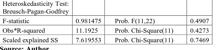
4.5.4 Heteroskedasticity Test ... 58
4.5.5 Regression Specification Error Test (RESET) ... 59
viii
4.7 Long-run relationship between external debt servicing and current account balance ... 62
4.8 The Responsiveness of the current account balance to changes in the external debt servicing... 66
4.8.1 Impulse response function (IRF) ... 66
4.8.2 Variance Decomposition Analysis (VDA) ... 67
CHAPTER FIVE ... 69
SUMMARY, CONCLUSIONS AND POLICY IMPLICATIONS ... 69
5.1 Introduction ... 69
5.2 Summary ... 69
5.4 Policy Implications ... 72
5.5 Areas for Further Research ... 73
References... 74
APPENDICES ... 80
APPENDIX 1: DATA ... 80
APPENDIX II: FIGURES ... 81
ix
LIST OF TABLES
Table 4.1 summary statistics for selected macroeconomic variables...46
Table 4.2 Unit Root Tests Results...53
Table 4.3 Cointegration results...55
Table 4.4 Multicollinearity results...57
Table 4. 5 Breusch-Godfrey Serial Correlation LM Results...58
Table 4. 6 Heteroskedasticity Test Results...58
Table 4. 7 Ramsey Test Results...59
Table 4. 8 Granger causality Results...61
Table 4.9 Regression Results...63
Table A1.1 Refined data...80
Table A1.2 The residual normality test...85
Table A1.3 Lag length selection results...86
Table A1.4 VECM estimation results...87
x
LIST OF FIGURES
Figure 1.1 Trend of current account Balance in Kenya, 1980-2015...4
Figure1.2. Current account balance of selected East African Countries....…...6
Figure 1.3 Trend of external debt servicing and current account balance ……...8
Figure 4.1 (a) Distribution curve for CAB ...49
Figure 4.1 (b) Distribution curve for EDS ………49
Figure 4.2 Multiple box plots for the variables...51
Figure A1.1 Histogram with superimposed normal curve for CAB...81
Figure A1.2 Histogram with superimposed normal curve for EDS...82
Figure A1.3: CUSUM Stability Test Result...79
Figure A1.4: CUSUM of squares Stability Test Result...84
xi
ABBREVIATIONS AND ACRONYMS ADF Augmented Dickey Fuller
AfDB African Development Bank
AIC Akaike Information Criterion
ARDL Autoregressive distributed Lag
BoP Balance of payments
CAB Current account balance
CAD Current account deficit
CBK Central Bank of Kenya
ELGS Exports Led Growth Strategies
EPZ Exports Processing Zones
HIPCs Heavily Indebted Poor Countries
IDA International Development Association
IMF International Monetary Fund
ISS Imports substitution strategy
KNBS Kenya National bureau of statistics
OLS Ordinary Least Squares
xii SSA Sub-Sahara Africa
TOT Terms of Trade
VAT Value Added Tax
VAR Vector Autoregressive
xiii
OPERATIONAL DEFINITION OF TERMS
Balance of payments: It is a summary statement that summarizes a country’s transaction with the foreign countries (rest of the world). It comprises the capital account, financial account and the current account.
Current Account Balance: It is the sum of three components: the trade balance, unilateral transfers such as foreign aid and the factor income balance such as interest and dividends
Current Account Deficit: Current account deficit implies that country’s export of goods and services is less than the value of goods and services imported.
External debt: This is the debt owed to external creditors. These creditors include: International Development Association (IDA), World Bank (WB), African
Development Bank (AfDB), International Monetary Fund (IMF) and other
international institutions.
External debt Servicing: This is the sum principal repayment, interest charged on the debt and any late payment fees. It can be paid in currency, services or goods.
Vector Auto regression: It is a forecasting technique in economics that does not distinguish between exogenous and endogenous. It treats all variables systematically without imposing any restriction to the system.
Debt overhang effect: It happens when there is some probability that in future, debt will be bigger than the country's reimbursement capacity where expected debt
xiv
Debt Burden: when the cost of servicing external debt is too high due to large external debt portfolio.
Causality: When the future value of a variable can be predicted by past values of another variable
Liquidity constraints theory: This is putting limit on the amount an individual can borrow or alteration in the interest rate the borrower should pay therefore raising the
xv ABSTRACT
1
CHAPTER ONE
INTRODUCTION
1.1 Background
Constant current account imbalances in many developing nations has energized extensive enthusiasm among economists and policy makers looking to have clear understanding of the significance of current account balance in macroeconomic issues. Many countries have run huge and constant current account imbalance which have been followed by economic slowdowns and severe financial crises (Kariuki, 2009). Current Account Balance (CAB) is one of the components of the Balance of Payments (BoP) in open economy (Mwangi, 2014). The other components are capital account and financial account.
1.1.1 Balance of Payments
Kenya’s balance of payments which summarizes Kenya’s transaction with the
foreign countries decreased into a deficit of Ksh 6 billion in the year 2015 from Ksh 5.18 billion in 2014 (CBK, 2015). This was contributed by a drop in financial inflows and low number of tourists which wiped out gains of a lower import bill. This meant that Kenya had more outflows than the inflows (receipts). This negatively affected the shilling, which depreciated by 13 percent the same year. The deficit resulted from Ksh 8.4 billion increase in the capital account surplus that could not offset 37.5 percent decrease in the financial account surplus.
2
countries to pay for its imports. In the short-run a deficit in the balance of payment fuels the country's economic growth because the country can use part of the borrowed funds to finance government projects that generates income (IMF, 2009). In the long-run, the country becomes a net consumer of the world's economic output. Since the country is now consuming products of the other countries it will have to go into debt to pay for consumption. This means that the country will not be investing in future growth. If the deficit continues long enough, the country may sell its assets such as natural resources, land and commodities to pay the creditors. On the other hand a balance of payments surplus means the value of country imports is less than the value of its exports. A surplus in the balance of payments boosts economic growth in the short term because the country lends money to countries that buy its products.
Balance of payments comprises of three components namely: the financial account, the capital account and the current account. The capital account captures the financial transactions that don't affect economic output while the financial account captures the change in international ownership of assets. Current account balance (CAB) which is the main component captures the trade balance (net export), unilateral transfers such as foreign aid and the net factor income from abroad such as interest and dividends. CAB which also represents the difference between domestic saving and investment is a key economic indicator of how a country is performing externally (Giancarlo, 2002). Current account balance constitutes an integral measure of national saving and therefore it can be used as an indicator of a country’s saving and spending
3
income. CAB plays a leading role and it is an important factor in policy formulation, analysis and decision-making processes in the increasingly interdependent world economy (Edwards, 2001).
Economic theory contends that whether current account imbalance is beneficial or detrimental to the economy depends on the factor that gave rise to it (Ghosh and Ramakrishnan, 2006). Generally, large persistent current account imbalance may signal ill-performance and vulnerability of the economy (Todaro and Smith, 2003). Persistent current account imbalance is also a key indicator of low national savings and investments, lack of international competitiveness and structural economic problem such as an undeveloped financial system. Furthermore, current account imbalance means a potential loss of output, increased unemployment and unbalanced economic growth (Nusrate, 2008; Ogwuru, 2008; Ghosh and Ramakrishnan, 2006).
In Kenya the import export gap grew by nearly 33 percent in the year 2002 due to the country importing machinery and other capital goods for infrastructure projects. This led to high current account deficit during the same year. Although the deficit was contributed by investment in transport projects, which will be paid off economically after their completion, there was high likelihood that this deficit was one of the main causes why the shillings depreciated during the same period (Mwenga, 2007).
4
influence the investment, national saving, and fiscal performance among other macroeconomic variables. These are some of the key factors that will influence the current account position. This is the fundamental motivation behind the current account balance research.
1.1.2 Trend of the Current Account Balance (CAB) in Kenya, 1980-2015 The current account balance in Kenya has been in deficit for the entire period under study. Although the deficit in the current account might be something good when it quantifies the investment finance gap that should to be filled up, it can also represent a dangerous and unsustainable imbalance between national investment and national savings and therefore lead to accumulation of external debt.
Figure 1.1 Trend of current account balance in Kenya, 1980 to 2015
Source: International Monetary Fund: World Economic Outlook Database, 2015
Figure 1.1 shows the trend of current account balance in Kenya for the period between 1980 and 2015. The figure reveals that current account balance in Kenya
-20 -15 -10 -5 0 5
1970 1980 1990 2000 2010 2020
C
A
B
(%
G
D
P)
YEARS
CAB(% GDP)
5
was unstable between 1980 and 2015 with current account deficits dominating the scene. Patterns in current account deficit in Kenya have been increasing to the tune of 18.7 percent of GDP in 1998 as shown in figure 1.1. In the year 2012 the current account deficit stood at 13.1 percent of the gross domestic product. There is a concern that since 2003, the upward pattern in growth of the current account deficits has proceeded unabated.
The depicted instability could be attributed to several factors that include internal and external shocks. The deteriorating terms of trade for the country’s exports
and the world recession in the early 1980s, had adverse impacts on the economy (Republic of Kenya, 1982). In the period 2010/2015 the deficit increased to the tune of US$ 6.08 billion due to investments in infrastructure-related imports. This trend is a concern to economists and policy makers because the health of a nation's external balance is shown by the current account balance among other factors. The essential indicator of macroeconomic crisis is the current account imbalance in form of actual or anticipated current account deficit (Summer, 1996).
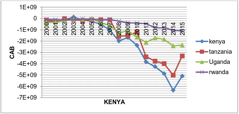
1.1.3 Current account balances of selected East African countries
6
Figure 1.2 Current account balances of selected East African countries Source: International Monetary Fund: World Economic Outlook Database, 2015 Figure 1.2 shows the trend of current account balances of different countries in East Africa. It is observed that Kenyan current account balance has been worse compared to other countries in East Africa. This unfavourable trade scenario has been exacerbated by the fact that Kenya’s exports are dominated by few primary
commodities, which have low price and income elasticities. Generally, Kenya is a net-importer. Various trade policies have been put in place to address this persistence current account deficit. Some of these policies are import substitution, liberalization of trade through Structural Adjustment Programmes (SAPs), exports led growth policies and current multilateral trade agreements. The import substitution strategies were aimed at industrialization through promotion of infant industries.
Administrative measures including licensing of importation, tariffs and price regulations were adopted in the 1980s. These policies failed to bear results as far as reducing the current account deficit was concerned (Were, 2007). In the 1980sKenya shifted from imports substitution strategy (ISS) and adopted exports led growth strategies (ELGS) under the structural reforms. This was caused by
-7E+09 -6E+09 -5E+09 -4E+09 -3E+09 -2E+09 -1E+09 0 1E+09
2000 2001 2002 2003 2004 2005 2006 2007 2008 2009 2010 2011 2012 2013 2014 2015
C
A
B
KENYA
7
pressure from the multi-lateral financial institutions to address deteriorating exports. As a result the current account deficit improved during the same period. The export promotions strategies put in place included the Export Processing Zones (EPZs) and the implementation of Export Trade Authority. As a result EPZs were subjected to a tax holiday for a period of ten years starting from that time and import duty exemptions on processing equipment for investments.
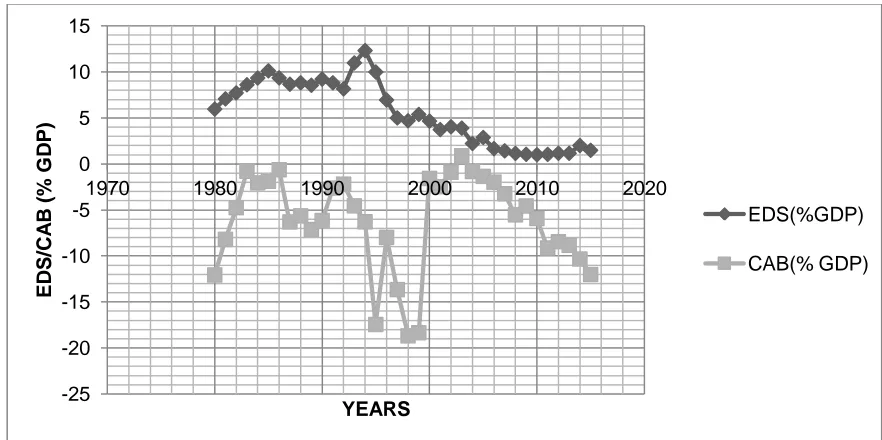
1.1.4 External debt servicing and current account balance in Kenya
8
Figure 1.3 Trends of external debt servicing and current account balance as a percentage of GDP
Source of the basic data: International Monetary Fund (IMF): World Economic Outlook Database, 2015
Figure 1.3 shows that the external debt servicing and current account balance in Kenya have been fluctuating from 1980 to 2015. The highest external debt service in 1994 was followed by a huge current account deficit in 1995. Figure 1.3 reveals that a current account surplus in 2003 was followed by the lowest external debt service in 2004. A critical look at Kenya’s fiscal scene reveals an expansionary fiscal phase indicated by an increase in the primary deficit. These fiscal developments have resulted to an increase in the share of debt service in total spending over the years. This is due to accumulating debt stock, which increases servicing amounts. For instance, external debt servicing rose from 8.1 percent to 12.3 percent of recurrent spending, equivalent to 4.2 percent of GDP between 1993 and 1994. In 2014/15, external debt servicing without factoring in debt redemption, amounted to Ksh 121.4 billion, representing 2.8 percent of the GDP. This means that external debt servicing was consuming a big share of
-25 -20 -15 -10 -5 0 5 10 15
1970 1980 1990 2000 2010 2020
9
budgetary allocations. This increase in external debt service was attributed to both external and internal factors.
In the mid-1980s the world loan fees expanded pointedly as an outcome of anti-inflationary programmes in the industrialized nations (Republic of Kenya, 1982). In the meantime, the terms of trade weakened for the borrower world as raw material costs fell. Kenya’s growth of exports earnings declined from 26 percent
in 1980 to 13 percent in 1981. Due to debt write-offs and a decline in bilateral and private debt the growth of external debt in 1988 and 1989 declined. Further In 1989, Kenya was forgiven its external debt amounting to US$463 million.
The decline in the 1990s was attributed to the fact that there were no new external debt contracts due to aid embargos and negative net-repayments. The two-year 'help freeze' in official capital inflow in 1991 and 1992 brought about an expansion in Kenya's external instalment overdue debts (Magero, 2015). Further there was likewise substantial dependence on domestic borrowing in relation to external borrowing in the 1990s and a generally tight financial position was additionally seen during the period. Kenya serviced its external debts without rescheduling despite the magnitude of external debt. This is also confirmed by the fact that there was negligible or zero accumulation of arrears in 1970s and a better part of 1980s (Mutai et al., 2008)
10
falling (Magero, 2015). Although Kenya may not have huge debt as compared to other heavily indebted poor countries (HIPCs), her present poor economic performance and inability to meet her debt obligations have serious implications on economic development. Other factors which led to high external debt included an overvalued exchange rate, import-substituting industrial strategy, and negative real interest rates which were characterized by overprotection. The more prominent pervasiveness of the import authorizing framework and regulations on business exercises made enormous opportunities for rent-seeking and for official discretion (Magero, 2015).
1.2 Statement of the problem
Current account balance in Kenya has remained beneath what economists would consider feasible. When the current account balance of a country remains in deficit for an extended period, it raises concerns about the sustainability of this deficit (Summer, 1996). As a rule of thumb, current account balance below-5 percent of GDP is alarming especially if funded by short-term debt or foreign reserves (Kenen, 1995). In 2014, the current account balance in Kenya stood at - 8.5 percent of GDP and -10.3 percent in 2015. Current account balance in Kenya is below the world average current account balance which stood at -3.5 percent of the GDP by the year 2015. Kenya has not just operated with current account balance surpassing -5 percent for the greater part of the years in her history, but the current account deficits have likewise shown some volatility.
11
its ability to repay the debts is becoming questionable (Mutuku, 2016). This is on the grounds that solvency requires that the nation be willing and able to produce adequate current account surpluses to reimburse what it has borrowed to finance the current account deficits.
The bulk of empirical studies have focused on the relationship between current account balance and key macroeconomics variables in various countries yielding different results. For instance Mbanga and Sikod (2008) found a unidirectional causality between external debt servicing and current account balance. However, Kayikci (2011) revealed existence of bidirectional causality between current account balance and external debt servicing. Blanchard and Francesco (2002) found that an increase in external debt servicing will have a positive impact on current account balance but Hermann and Jochem (2005) revealed that external debt servicing affected current account balance negatively. The review of these empirical studies has shown that it is inadequate to generalize the link between external debt servicing and current account balance. Studies such as Mutuku (2016); Mwangi (2014) and Kariuki (2009) yields mixed results about the factors that impact the movement of current account balance in Kenya.
12 1.3 Research Questions
The study provided answers to the following questions:
(i) What is the nature of causality between external debt servicing and current account balance in Kenya?
(ii) What is the long run relationship between external debt servicing and current account balance in Kenya?
1.4 Objectives of the Study
The general objective of the study was to investigate the relationship between external debt servicing and current account balance in Kenya.
The specific objectives of the study were:
(i) To determine the nature of causality between external debt servicing and current account balance in Kenya.
(ii) To determine the long run relationship between external debt servicing and current account balance in Kenya.
1.5 Significance and Scope of the Study
13
the period 1980 to 2015. The period was considered to be long enough to capture the relationship between the external debt servicing and current account balance.
1.6 Organization of the study
This project is exhibited in five chapters. The foregoing chapter introduced the study and its objectives. It has additionally given background information of the current account balance and external debt service. Chapter two involves a review of both theoretical and empirical literatures that are relevant to the study. Chapter three gives the methodology that was adopted; it includes the research design,
14
CHAPTER TWO LITERATURE REVIEW
2.1 Introduction
This chapter presents relevant theoretical and empirical literature which forms the grounding for investigating the relationship between external debt servicing and current account balance. Finally the overview of the literature and research gaps is discussed.
2.2 Theoretical Literature
In this section, a review of major theoretical arguments regarding current account balance is done.
2.2.1 Elasticity approach
One of the most important neoclassical theories that are applied in analysis of current account balance (CAB) is the elasticity approach developed by Thirlwall in 1986. The theory holds that current account balance disequilibria are caused by lack of competition in the international market. According to this theory current account depends on income elasticities and price of goods. According to this theory CAB can be defined as:
CAB = X.P - ePf.M ……….2.1
Where:
X is the exports
P is the domestic price
15 M is imports and
e is the exchange rate.
The exchange rate is expressed as the ratio of domestic price and foreign price as shown in equation 2.2 below:
e = P/Pf……….……2.2
Equation 2.2 shows that the value of exchange rate (e) increases as the value of domestic price (P) increases and it decreases with decrease in foreign price (Pf).
With the assumption of given prices, equation 2.1 can be rewritten as:
CAB = X – eM……….…………..2.3
Differentiating equation 2.3 with respect to exchange rate (e) the following equation is obtained:
Dividing equation 2.4 through by M the following equation is obtained:
But export and import elasticities can be defined as follows:
16
Inserting equation 2.6 in to equation 2.5 it yields the following equation:
Assuming that the current account is in balance and therefore X = eM, then:
M = X/e……….……….…….2.9
Inserting equation 2.9 in to equation 2.8 and rewriting the resultant equation yields the following equation:
Inserting equation 2.7 into equation 2.10 and rewriting the resultant expression the following equation is obtained:
But since CAB should improve with devaluation, then it follows that:
If equation 2.12 holds then
Equation 2.13 satisfies the Marshall-Lerner (ML) condition, which states that for currency depreciation to improve the current account balance the sum of price elasticities of exports and imports must be greater than unity (Mudida, 2012).
17
so that a variation in nominal exchange rate causes a proportionate change in real exchange rate (Giancarlo, 2002).
2.2.2 Debt overhang theory
The debt overhang theory first discussed by Myers in 1977 depends on the fact that
if debt will surpass the nation's repayment ability with some likelihood in the future, then the expected debt service is likely to be increasing as the country’s output level increases. In this manner a portion of returns from investing in the domestic economy will be taxed away to pay the existing creditors and this will discourage new foreign investors (Claessens, Detragiache and Kanbur, 1996). The borrower country will therefore use only partially of any increase in output and exports since a good portion of that increase will be used to service the existing external debt. This creates a problem because if a country has a new investment project which may generate positive net present value, the country will not invest due to an existing debt position hence the country’s level of investment will start
decreasing.
18
government spending. According to intertemporal approach of the current account balance (CAB):
CAB = (S-I) + (T-G) ---2.14
Where:
S is domestic saving
I is investment
T is taxes and,
G is the Government spending.
From equation 2.14 it is clear that increase in the level of investment will worsen the current account balance while reduction in government spending will improve the current account balance (Elbadawi et al., 1996). Referring to this theory Lensink and white (1999) argued that external debt may be beneficial or detrimental to economic growth. According to Lensink and White there is a threshold at which more external debt is detrimental to economic growth. External debt affects the economy positively until a certain point but beyond this point the effect becomes negative (Lensink and white, 1999).
2.2.3 Liquidity constraint hypothesis
19
service debt reduces funds available for investment and growth (“Crowding out” effect). Reduction in the debt service will therefore lead to an increase in current investment and thus worsen current account balance (Cohen, 1993). The need to service large amount of external debts can affect economic performance due to lack of access to international financial markets (Claessens et al., 1996).
2.2.4 Balance of Payment Constraint Model
Balance of Payment constraint model formulated in 1986 by Thirlwall adopted a Keynesian view of aggregate demand and output but fundamentally incorporates the neoclassical elasticity approach in its formulation. This model otherwise known as Thirlwall Law has gained a lot of popularity. According to this theory, export is the only components of national output that provides foreign reserves which consequently allows the growth of other demand components in an open economy (Bahmani and Ratha, 2004). BoP constraint model explains that if an economy’s rate of imports exceeds the rate of exports then current account
deteriorates which in turn impedes economic growth.
BoP constraint model holds that faster income growth relative to export growth may only cause balance of payment disequilibrium because it increases demand for imports relative to export thus worsening the current account position. According to this model increase in external debt will increase the demand for imports which will worsen the current account.
20
growth increases productivity which further increases competitiveness and revenue growth from exports (Bahmani and Ratha, 2004).
2.2.5 The Absorption Approach
The absorption approach was developed by Murshed (1997). According to this theory the difference between domestic output and spending (absorption) represents the current account balance. If income is greater than absorption there would be a trade surplus and vice versa. The theory emphasizes on changes in real domestic income and therefore it is referred to as real-income theory of the balance of payments (Kosimbei, 2002). The theory assumes that prices remain constant. It is based on Keynesian national income framework which is given as:
Y = C+I+G+X-M---2.15
Where:
C is Consumption
I is Investment
G is Government expenditure and
Y is Output.
Absorption (A) which is also known as aggregate spending is given as:
A = C+I+G---2.16
Substituting the absorption equation 2.16 into equation 2.15 and rewriting the resultant equation yields the following equation:
21
Current account balance (CAB) is defined as a sum of three components: the net export, net current transfers and the net income from abroad.
CAB = X-M +NI+ CT ---2.18
Where:
X and M are Exports and imports respectively.
NI and CT are net income from abroad and net current transfers respectively.
Net incomes from abroad (NI) and net current transfers (CT) are assumed to be very small and negligible for the case of Kenya (Njoroge, 2014), hence they can be dropped from equation 2.18 yielding the following equation:
CAB = X-M ---2.19
Substituting the current account balance equation 2.19 into equation 2.17 and rewriting the resultant expression yields:
CAB = Y –C–I–G ---2.20
From equation 2.20 it is clear that factors that affect consumption, investment and government expenditure will indirectly affect current account balance.
2.3 Empirical Literature
22
directly affect the economic growth but it influences economic growth through the accumulated external debts as a proportion of GDP and the past debt accumulation as a proportion of the debt service. The empirical outcomes demonstrated the existence of negative relationship between external debt and economic growth in Kenya. Further the negative relationship between private investment and external debt also known as the crowding out effect was confirmed. This confirmed the existence of debt overhang problem in Kenya since debt service caused crowding out effect. However, this study did not show how this crowding out effect affected the current account balance.
Blanchard and Francesco (2002) documented the ways through which financial integration can affect the position of current account balance using autoregressive distributed lag (ARDL) model. With increasing financial integration the cost of borrowing is expected to decrease. The developing countries with lower level of capital, high growth prospects and higher marginal productivity will increase their external borrowing to finance domestic investment. This will affect their current account balance negatively. The study established the relationship between various macroeconomic variables and current account deficit in Sub-Saharan Countries. The study revealed that there was a positive significant coefficient of 0.1067 between external debt and current account balance which implies that an increase in external debt by one unit will increase the current account balance by 0.1067 units. However, the study employed panel data for various Sub-Saharan nations and therefore the results cannot be used to address the specific issues in Kenya.
23
grouping. The study applied panel regression techniques in analysing the data for different country grouping. The study revealed that current account balance of non-oil developing countries is affected by both external and internal factors. The study indicated that external debt servicing and current account balance were negatively related. The findings of the study revealed that, a unit increase in external debt servicing led to 2.523 percent decline in current account balance. This implied that accumulation of external debt worsens the current account position. Further the study revealed that external debt affected current account balance through high interest payments. The study also showed that 2.15 percent of fluctuations to current account were caused by the rate of inflation. The study used panel data for various countries and suggested that an empirical analysis should be done in each country to determine the effectiveness of current account determinants.
24
Mbanga and Sikod (2008) analysed the impact of debt and its interest repayment on macroeconomic variables in Greece. Using vector autoregressive (VAR) the study pointed out that the external debt servicing and the rate of inflation greatly affected the current account developments during 1995-2006 in Greece. Further the study established a negative relationship between budget deficits and current account balance. The main assumption of the study was that stationary current account series ensured the long-run relationship and therefore the study assumed that the current account balance could also have unit roots (non-stationary). The study used Markov-switching –Augmented dickey fuller econometric framework and pointed that reduced debt burden and low rate of inflation increases the degree of current account balance persistence.
Mutai et al. (2008) studied the effects of external debt servicing on economic growth in Kenya using secondary data for the period between 1996 and 2007. The study used generalized method of moment’s regression model. The variables
used in the study included the lagged values of GDP, broad money supply, ratio of government expenditure to GDP, secondary school enrolment, ratio of debt to GDP and the private sector credit. The study confirmed the existences of crowding out effect where by the private investment were crowded out by the external debt due to high interest repayments. Crowding out of private and public investment led to a decrease in government spending and national income which worsen the current account balance.
25
influenced by terms of trade. The results revealed that if terms of trade increased by 1 per cent current account balance increased by 0.11 percent holding other factors constant. Further the study pointed out that the relationship between real exchange rate and current account balance was positive. The other factors which affected the current account balance negatively included the foreign direct investments and external shocks. However the study ignored many factors that influence the current account balance movements. The study suggested that taking care of causality consequences, a similar study should be carried out using dynamic modelling that aims at examining impulse responses
Morsy (2009) investigated the relationship between current account balance and currency crisis in oil exporting countries using Intertemporal Approach. The study revealed that external debt among other factors influenced the position of the current account balance. The study used panel data for different oil exporting countries. Unit root test revealed that current account balance was a stationary series in the period and therefore co integration methods were not appropriate. The study therefore applied generalized methods of moments (GMM) which controls for endogeneity and corrects for the bias. The choice of this method was supported by the fact that the dependent variable was lagged and could affect estimation. The study established a negative relationship between external debt burden and current account balance since 1 percent increase in external debt burden will lower the current account balance by 0.35 percent.
26
service. The results established bidirectional causality between current account balance and external debt service. This confirmed the hypothesis that the values of current account balance can also be used to predict the values of external debt service. It was established that 40 percent of variations in current account balance were caused by innovations in current account balance (past) and 26 percent of the variations were caused by external debt service. Variations in Current account balance were also highly influenced by the innovations in investment to GDP ratio and real exchange rate.
Mwangi (2014) utilized quasi experimental research design to empirically investigate current account determinants in Kenya using secondary data for the period between 1970 and 2010. The study applied the vector auto regression (VAR) model and established that current account balance was positively related to: gross domestic product, financial deepening, savings and real exchange rate. Current account was negatively influenced by investment, rate of inflation and balance of trade. It was established that Kenya being a unique economy, the issue of current account is very tricky. The exchange rate was established that highest impact on the current account amounting to 17.97 percent in long run. The results show that investments and savings have mild effect on the current account balance in Kenya. This is attributed to the fact that the savings and investments are affected by other macro-economic variables.
27
innovations in total debt servicing would persist in the economy for over ten years to shrivel. However the focus of this study was limited to effect of total debt service on few selected macroeconomic variables which included gross domestic product (GDP), private investment (PI) and real exchange rate (RER). The study ignored other macroeconomic variables and proposed further investigation on the relationship between debt servicing and all other macroeconomic variables.
Mutuku (2016) applied the vector error correction model (VECM) to analyse current account determinants in Kenya. Current account balance, GDP growth rate, dependency ratio, trade openness, net foreign asset, national income, oil prices and real exchange rate were used as the variables in the model. The study established that gross domestic product and trade openness had the greatest positive impact on current account on the first year. Net foreign asset, fiscal balance, oil prices, real exchange rate, dependency ratio and output level had negative effect on current account balance. The results on long run co-integrating model reveal that financial deepening in Kenya has no effect on the current account balance at 5 percent, 10 percent and 1percentlevel of significance. Since the study was limited to selected macroeconomic and demographic factors on current account balance, it suggested that a country specific study on the dynamic effect of monetary and fiscal policy shocks on balance of payment components would be useful in informing policy in this area.
2.4 Overview of literature review and research gaps
28
representing the unpredictability of relationships between macroeconomic variables. Studying these literatures reveal conflicting and inconclusive evidence that raises doubts about the nature of the relationship between these macroeconomic variables. For instance Mbanga and Sikod (2008) found a unidirectional causality between external debt servicing and current account balance in Greece. This was in support of Morsy (2009) which found that external debt service granger causes current account balance. However, Kayikci (2011) revealed existence of bidirectional causality between current account balance and external debt servicing. Kayikci (2011) found that current account balance can be used to predict external debt service which was in conflict to Mbanga and Sikod (2008) and Morsy (2009).
29
30
CHAPTER THREE METHODOLOGY
3.1 Introduction
This chapter presents the methodology that was utilized in the study. It incorporates the research design, theoretical framework, model specification, description of variables, the type of data used and the method of data analysis.
3.2 Research Design
The main objective of this study was to establish the relationship between external debt servicing and current account balance in Kenya. Non experimental research design which uses economic models for analysis was utilized. This design is mostly used in predictive research to predict the future status of dependent variables. Annual time series data was used in the study to answer the research questions posed in the first chapter.
3.3 Theoretical model
31
CAB = Y-A ---3.1
Where Y is output and A is absorption.
Absorption (A) which is also known as aggregate spending is given by equation:
A = C+I+G---3.2
Where:
C is Consumption
I is Investment and
G is Government spending
Inserting equation 3.2 into equation 3.1 yields:
CAB= Y-C-I-G ---3.3
The behavioural equations for the components in equation 3.3 can be written as follows:
---3.4
---3.5
---3.6
G = ---3.7
Where
Y is the level of output
32 T is the Tax revenue
I is Investment
is exogenous investments is interest rate
G is exogenous government expenditure (G*) and a, b, and are coefficients.
Substituting the behavioural equations into equation 3.3 and rearranging the resultant yields the following equation:
Budget deficit can be defined as the difference between government revenues and expenditures. With an assumption that the government`s total income is derived from taxes, then is equal to the deficit
Budget deficit (BD) can therefore be specified as:
Substituting equation 3.9 into 3.8 results into:
33
obligation the government public spending on infrastructure decreases. When countries are paying their external debt, they use their income from export to service the debt and thus reducing the funds available for imports.
Other factors have been identified from the previous chapter; they include rate of inflation (INF), terms of trade (TOT), nominal exchange rate (NER) and real gross domestic product (rGDP). The empirical model for this study was expressed in general form as:
CAB= f (INF, EDS, , , NER, rGDP, BD) --- 3.11
3.4 Empirical Model specification
The Study utilized vector Auto Regressive (VAR) model. VAR model does not impose restrictions to the system but treats all the variables systematically (Sims, 1980). This is because there are insufficient macroeconomic theories linking the above variables and therefore Ordinary Least Squares (OLS) technique will not be applicable.The compact form of a VAR model that link current account balance and external debt service among other explanatory variables in equation (3.11) took the form:
………… ...3.12
Where by is n × 1 vector of constant coefficients, is a n×1 vector of the selected endogenous variables (CAB, INF, EDS, TOT, , NER, rGDP, BD) and is a disturbance terms with a constant variance and Zero means. For example
34
Before the model was estimated the information criteria like Akaike Information Criterion (AIC) and Schwarz Information Criterion (SIC), Likelihood ratio (LR), and Final Prediction Error (FPE) were employed to decide the proper lag length for the VAR model.
The LR test was based on equation:
lnr lnu )~2(q)……….3.14
Where: T is the observations (after accounting for lags), M is the number of
parameters estimated in each equation,lnr is the natural log of the determinant of the covariance matrix of residuals and q is number of the restrictions in the system
The information criteria (AIC and SIC) are not tests that choose the lag that minimizes the criteria, they only indicate goodness of fit of alternatives and therefore they were only employed as complements to the LR tests. The AIC and SIC were based on the following equations:
N T
AIC ln2 ………...…3.15
T N T
35
Where T is the observations (after accounting for lags) and N is the number of parameters estimated in each equation of the unrestricted system.
The cointegrating test results confirmed that there was cointegration and thus the relationship between the variables could be described by restricted VAR also known as Vector Error Correction model (VECM). A vector error correction model (VECM) is a restricted VAR that has cointegration limitations incorporated with the determination, so that it is intended for use with non-stationary series that are known to be cointegrated. The VECM specification limits the long-run behaviour of the endogenous variables to converge to their cointegrating relationships while permitting an extensive variety of short-run dynamics. The cointegration term is known as the error correction term since the deviation from long-run equilibrium is amended gradually through a series of incomplete short-run modifications. The general vector error correction model with deterministic trend is:
……….. 3.17
Where
To estimate the equation 3.17 the equation was further rewritten as:
+ ………. 3.18
36 3.4.1 Granger Causality Test
X is said to Granger-cause Y if the future values of Y can be better determined utilizing the past values of both X and Y than it can by utilizing the past values of Y alone (Giles, 2011). The study tested for existence of causality between the economic variables using the granger causality test. This is a test which checks if one time series could be used to predict another time series (Engle and Granger, 1987). To examine Granger causation between external debt service and current account balance the granger causality test was done through estimation of two regression equation expressed as follows:
9
The joint hypothesis of F-test based Wald statistics for equation 3.19 and equation 3.20
3.4.2 The Long Run Relationship
37
From equation 3.13Let = CAB and Xt represents all the explanatory variables
Where is the of the past values of Y up to lag m and is the sum of the past values of right hand side variables up to lag m and their coefficients.
Rearranging equation 3.21 and expanding the terms yields equation 3.22
22
Introducing lag operator in equation 3.22 yields:
...3.23
Factoring and from equation 3.23 yields the following equation:
+
...3.24
If it is assumed that in the long run, and are constant, then equation 3.24 can be rewritten as:
+ ………..………3.25
Where and long run coefficients of the long run equations defined as:
38
…...3.27
Specifically the long run equations estimated were expressed as follows:
3.4.3 The Dynamics Response
Studies have found that estimated coefficients of the VAR model have no economic interpretation because they are in form of reduced equations. Sims (1980) came up with a method of estimating VAR coefficients to trace the dynamics path of a specific variable in a system, given a certain effect of innovation or a shock brought about by a change in a variable.
The dynamic response is estimated through variance decomposition and the impulse response functions (IRFs). The effects of shocks to the system will be summarized by use of impulse responses functions. The impulse response functions will allow the determination of the signs of the effect of innovations or external change in each variable on others. IRF involves measuring unexpected changes in one variable (the impulse) in time t and then predict its effect on the other variable in time t, t+1, t+2… t+n (the responses). The IRF was based on
equation:
39
Where yt is a vector of the considered dependent variables, εi is a vector of
innovations for all variables that have been included in the model, α is a vector of the constants, and Θi is a vector of parameters that measure the reaction of the
dependent variable to innovations in all other variables included in the model. Taking two specific variables Yt and Xt to represent CAB and EDS respectively,
the IRF was expressed as follows:
Where by φ’s and ’srepresent the amounts of responses
Equations 3.31 and 3.32 express how the dependent variable responds to previous innovations that happen to the endogenous variables included in the model. 3.4.4 Variance Decomposition Analysis
The variance decomposition analysis measures how important the error in the jth equation is for explaining unexpected movements in the ith variable (Enders, 1995). Variance decomposition tells how much of a change in a variable is due to its own shock and how much is due to shocks to other variables. In the short run a large portion of the variation of a variable is due to its own shock. The variance decomposition analysis was derived as follows:
In calculating the n-period forecast error of x in order to find that of y, equation 3.33 was utilized.
40
Considering variable y which is the first element in the x matrix then the p-step forecast error is
) ...
( ,0 , ,1 , 1 , 1 ,1
n t n n yt nn yt n nn yt t Ey
y
+
...3.34
3.5 Definition and measurement of variables
Current account balance (CAB): This is the value of Kenya’s net exports of goods and services in one year. Grants were excluded because their inclusion will
give biased results. In this study it was expressed as percentage of gross domestic
product (GDP)
Inflation rate (INF): This is general change in prices paid by consumers over a given time. It was measured by the recorded inflation rate for the given year. Rate
of inflation in year t = {(Prt – Prt-1) / Prt-1}*100
Where Pr is the price and t is the time frame.
External debt Servicing (EDS): External debt service is the payments of both principal and interest charged on the external debt. It also included any late payment fees. It was standardized by expressing it as a percentage of GDP.
Terms of Trade (TOT): This is the difference between the prices of goods exported and the prices of goods imported. In this study 2000 was used as the
41
Interest rate (IR): Interest rate is the reward of parting with liquidity for a specified period usually one year. It was measured in percentage per annum by
taking the annual average.
Budget deficit: This is the value of Kenya’s Central government revenues net its expenditures in one year. In this study it was expressed as a percentage of GDP
Nominal Exchange Rate (NER): This is the price of a US dollar in terms of Kenya shillings given by annual average.
Real Gross domestic product (GDP): This is the monetary value of all the completed goods and services produced within a country’s borders within one
year. It was standardized by taking its annual growth.
3.6 Time series properties
The study tested for time series properties such as the presence of unit roots and cointegration before estimation. This was to guarantee meaningful regression results.
3.6.1 Stationarity test
The significance of this test was to model stationary series. This ensured that the
resultant regression results are meaningful. For a series to be stationary it should
have a constant mean and variance. To perform this test the study employed
Augmented Dickey Fuller (ADF) test procedure which was explained by Dickey
and Fuller (1976). The choice of ADF was supported by the fact that it retains the
validity of the tests. The non-stationary time series were then differenced until
they become stationary. To confirm the ADF test the Phillips-Perron (PP) test
42
serial correlation in the time series was employed. Philips-Perron test takes care
of the serial correlation in the error terms without adding lags by use of
nonparametric statistical methods. The ADF test involved estimating the
following three equations:
ADF without intercept and trend
35 . 3
1
1
t i t ni i t
t y y
y
(i) ADF with an intercept but no trend
36 . 3
1
1
t i t pi i t
t y y v
y
(ii) ADF with both the intercept and trend
37 . 3
1
1
t i t ni i t
t t y y
y
Where: is the intercept, tis the trend, i represents the number of lags in ∆yt-i
with the maximum being n and tis the random error term
The PP test involved the estimating equation 3.38
38 . 3 1
t i t mi i
t y e
y
Where yt is the first difference of the dependent variable, i represents the number of lags, β and α are the coefficients andtis the error term
3.6.2 Cointegration Analysis
43
(Greene, 2008). Thus, cointegration suggests that despite the time series being exclusively non-stationary, there is existence of a long run relationship between them. Cointegration makes it conceivable to capture relationship between non stationary time series inside a model which is stationary (Adam, 1988). The commonly used tests for Cointegration are Johansen’s method and Granger two-step methods (Engle and Granger, 1987). Johansen's methodology was utilized to test for Cointegration in this study since it licenses for more than one cointegrating relationship, unlike the Engle– Granger technique (Johansen, 1988). There are two test statistics (Trace and Eigen) used to test the number of co integrating vectors based on the characteristic roots. The trace test and maximum Eigen value test were computed as:
3.39
Where T was the sample size and was the ith largest canonical correlation. For both trace and the maximum Eigen value test, the null hypothesis was at most r cointegrating vectors. The alternative hypothesis for the trace test was at most k cointegrating vectors while the alternative hypothesis for the maximum eigen value test was at most r+1 cointegrating vectors.
3.7 Data type and source
44 3.8 Diagnostic tests
Diagnostic tests were undertaken to ensure consistent coefficient estimates. Various econometric tests such as Breusch-pagan test and Goldfeld-Quandt were conducted to test for heteroskedasticity and multicollinearity (Gujarati, 2004). Since some of the variables were lagged the study used Durbin’s h test to test for serial autocorrelation (Gujarati, 2004). The Jarque-Bera test was also conducted to test normality of the error term. This is a test that involved computing standard deviation, skewness, probability and kurtosis. This test is important in helping with the identification of presence of outliers. The VECM model was also tested for stability. In this regard, CUSUM tests and CUSUM of squares tests were used to test for model stability. This ensured consistent results as well as efficient results.
3.9 Data and analysis techniques
To achieve the two objectives presented in chapter one, the study utilized annual time series data for the period between 1980 and 2015. E-views econometric software was used to analyse the quantitative data collected. Various diagnostic tests were conducted to test for econometric problems in the data. Some of the diagnostic test included the problem of heteroskedasticity, multicollinearity and serial autocorrelation. To interpret the VAR model once it has been fitted Variance decomposition and impulse response functions (IRF) was used.
45
46
CHAPTER FOUR
EMPIRICAL FINDINGS
4.1 Introduction
This chapter presents the findings of the study. It gives the descriptive statistics and also the results of time series property test and diagnostic tests on the model estimated. The chapter also presents the findings and discussions on the relationship between external debt service and current account balance in Kenya. 4.2 Descriptive Statistics
The descriptive statistics reveal the salient features of the variables used in the study. The descriptive statistics helps one understand the nature of the variable one is dealing with. They include the measures of central tendency such as the mean and the median and also the measures of dispersion such as the standard deviation and the range. These statistics are presented in table 4.1.
Table 4.1 summary statistics for selected macroeconomic variables
CAB EDS INF GDP IR NER TOT BD
Mean -6.207 5.568 11.264 3.789 7.440 53.114 90.945 -4.361
Median -5.581 5.196 9.12 4.169 6.356 59.55 89.79 -4.15
Maximum 0.888 12.329 45.979 8.402 21.096 98.18 114.02 1.75
Minimum -18.67 1.004 1.554 -0.799 -8.009 7.42 70.15 -17.78
Std. Dev. 5.1420 3.516 8.517 2.333 6.695 29.234 10.347 3.77
Skewness -0.948 0.094 2.297 -0.18 0.069 -0.317 0.297 -1.302
Kurtosis 3.211 1.631 9.239 2.064 2.759 1.541 2.561 5.728
Jarque-Bera 5.465 2.863 90.0421 1.507 0.115 3.798 0.819 21.339
Probability 0.065 0.239 0 0.471 0.944 0.149 0.664 0.000
Sum -223.466 200.473 405.505 136.439 267.855 1912.09 3274.02 -157
Sum Sq.
Dev. 925.422 432.695 2538.779 190.455 1568.976 29911.52 3747.294 497.928
Observations 36 36 36 36 36 36 36 36
47
The average value of current account balance as a percent of GDP in Kenya was -6.207 percent against a target of -5 percent of the GDP. As a rule of thumb, current account balance below -5 percent of GDP is alarming especially if funded by short-term debt or foreign reserves. Current account balance in Kenya was below the world average current account balance which stood at -3.5 percent of the GDP by the year 2015. The minimum and maximum current account balance as a percent of GDP stood at -18.679 percent and 0.888 percent respectively during the same period. A standard deviation of 5.142 percent indicated a high variation from the mean during the period under study. The median current account balance of -5.582 percent as shown in table 4.1 which is not the same as the mean value of -6.207 percent indicates that the observations are not symmetrically distributed. The figures supported the study background that reveals that Kenya had instability in its current account balance with current account deficits dominating the scene and registering invisible current account surpluses.
48
3.516percent which showed that there was a very high variation from the mean. The median external debt service was 5.197 percent of GDP.
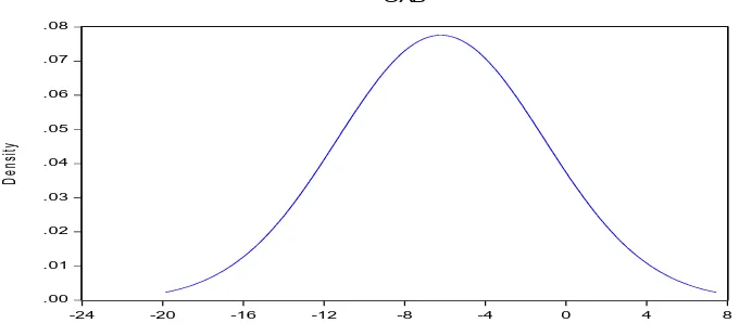
Table 4.1shows that current account balance was negatively skewed implying that the distribution had a long left tail. The same results are presented in Appendix II figure A1.1. On the other hand external debt service is positively skewed implying that the distributions have long right tail as presented in Appendix II figure A1.2.
Another observation from table 4.1 is the Kurtosis which is also known as the fourth moment. Kurtosis measures the peakedness or flatness of the distribution. Current account balance has a distribution with kurtosis >3 which is called leptokurtic. Compared to a normal distribution, its tails are longer and flatter, and its central peak is higher and sharper. This was further confirmed by histogram with superimposed normal curves in Appendix II figure A1.1.