DOI: 10.1017/S0022112002001982 Printed in the United Kingdom
On transonic viscous
–
inviscid interaction
By E. V. B U L D A K O V AND A. I. R U B A N
Department of Mathematics, University of Manchester, Oxford Road, Manchester, M13 9PL, UK
(Received 1 December 2000 and in revised form 10 June 2002)
The paper is concerned with the interaction between the boundary layer on a smooth body surface and the outer inviscid compressible flow in the vicinity of a sonic point. First, a family of local self-similar solutions of the K´arm´an–Guderley equation describing the inviscid flow behaviour immediately outside the interaction region is analysed; one of them was found to be suitable for describing the boundary-layer separation. In this solution the pressure has a singularity at the sonic point with the pressure gradient on the body surface being inversely proportional to the cubic root dpw/dx∼(−x)−1/3 of the distance (−x) from the sonic point. This pressure gradient
causes the boundary layer to interact with the inviscid part of the flow. It is interesting that the skin friction in the boundary layer upstream of the interaction region shows a characteristic logarithmic decay which determines an unusual behaviour of the flow inside the interaction region. This region has a conventional triple-deck structure. To study the interactive flow one has to solve simultaneously the Prandtl boundary-layer equations in the lower deck which occupies a thin viscous sublayer near the body surface and the K´arm´an–Guderley equations for the upper deck situated in the inviscid flow outside the boundary layer. In this paper a numerical solution of the interaction problem is constructed for the case when the separation region is entirely contained within the viscous sublayer and the inviscid part of the flow remains marginally supersonic. The solution proves to be non-unique, revealing a hysteresis character of the flow in the interaction region.
1. Introduction
being given by the Ackeret formula which establishes a local relationship between the induced pressure and streamline slope angle at the outer edge of the boundary layer. Transonic viscous–inviscid interaction may be observed, for example, in the flow past an aerofoil with small thicknessτin a uniform gas flow with the free-stream Mach number M∞ close to one. If the K´arm´an parameter K = (1−M∞2)/τ2/3 remains an order-one quantity asτ→0 simultaneously withM∞→1, then the entire inviscid flow around the aerofoil is governed by the K´arm´an–Guderley equations. Alternatively, the flow might become transonic only locally as the interaction region is approached. In both cases the behaviour of the inviscid part of the flow immediately outside the interaction region may be studied based on a self-similar form of the solution of the K´arm´an–Guderley equations. In the classical transonic theory such solutions were extensively used for the ‘far field’ analysis of the flow past aerofoils or slender bodies of rotation. If the free-stream Mach number M∞ = 1 then the solution of the Euler equations may be represented in the form
Φ(x, y) =x+ 1
γ+ 1y3k−2F0(ξ) +· · · as y→ ∞, with the similarity variable being
ξ= yxk.
Herexandyare appropriately non-dimensionalized Cartesian coordinates measured along and perpendicular to the unperturbed velocity vector in front of the aerofoil, and Φ is the velocity potential. The parameter k in this solution must be less than one to ensure that the perturbations vanish as the distance from the aerofoil increases (Cole & Cook 1986). As was found by Frankl (1947) and Guderley (1957), the corresponding ordinary differential equation for F0(ξ)
(F0
0−k2ξ2)F000−k(5−5k)ξF00+ (3−3k)(3k−2)F0= 0
has a non-trivial solution only for a particular value of the parameter k= 4/5. This solution involves a shock wave which was carefully investigated by Barish & Guderley (1953).
Our study is based on the observation that this same ordinary differential equation, but with k >1, may be used to analyse the behaviour of an inviscid gas flow in a vicinity of the sonic point on a rigid body surface. A local solution of this type was first given by Diesperov (1980) (see also Ruban & Turkyilmaz 2000) who considered a flow which accelerates towards a sonic point situated on a rigid body surface and separates from this surface as soon as the flow speed reaches the speed of sound. It was supposed that as a result of the separation a free streamline formed along which the pressure remained constant at least in a small vicinity of the separation point. The similarity solution that describes such flow behaviour exists if the parameter k is chosen to be
k = 6/5. In this solution the flow in front of the separation point is subsonic and its acceleration towards the separation point produces a favourable pressure gradient acting upon the boundary layer. Under these conditions the boundary layer cannot be expected to separate if the body surface is smooth. However, Diesperov’s (1980) solution proved to be well-suited for describing transonic flow separation from convex corners.
corner point. The pressure gradient generated in the inviscid transonic flow appears to be strong enough to cause a complete reconstruction of the boundary layer in front of the interaction region. The analysis in Ruban & Turkyilmaz (2000) revealed that the boundary layer splits into two parts, the near-wall viscous sublayer and the main body of the boundary layer where the flow is locally inviscid. Remarkably, the displacement effect of the boundary layer was found to be mainly due to the inviscid part of the boundary layer. Therefore contrary to what happens in similar subsonic (Ruban 1974) and supersonic (Neiland 1974) cases, the flow in the interaction region was found to be governed by the so called inviscid–inviscid interaction.
This example demonstrates that transonic interactive flows reveal their nature not just through the upper layer of the triple-deck structure where the K´a´rm´an–Guderley equations should be used instead of subsonic or supersonic interaction laws. More importantly the inviscid transonic flow in front of the interaction region proves to be capable of producing rapid variations in the flow field that might change completely the background on which the interaction between the boundary layer and external flow develops.
Earlier studies of transonic flows with the interaction were restricted to relatively simple situations when the flow outside the interaction region remains essentially unperturbed and does not influence the boundary layer approaching the interaction region. The first of these studies was performed by Messiter, Feo & Melnik (1971) who were concerned with viscous–inviscid interaction on the surface of a flat plate placed into uniform transonic flow. They found that for the transonic flow regime to hold the free-stream Mach number M∞ should be such that M∞−1 = O(Re−1/5), where
Re is the Reynolds number. The interaction region proved to be larger than at finite values of |M∞−1|. It extends along the plate surface over a distance ∆x∼Re−3/10 as compared to ∆x ∼ Re−3/8 for the corresponding subsonic and supersonic flows. Messiter et al. (1971) also noticed that the viscous–inviscid interaction problem could be significantly simplified if, firstly, the flow remains supersonic everywhere in the upper tier of the interaction region and, secondly, the inviscid flow is uniform immediately upstream of the interaction region. In this case the governing K´arm´an– Guderley equations admit a solution in the form of a simple wave analogous to the Prandtl–Meyer solution for supersonic flows. As a result a simple local (but nonlinear) interaction law is established relating the induced pressure to the streamline slope angle at the outer edge of the viscous sublayer.
Based on this formulation Brilliant & Adamson (1974) studied the process of the boundary-layer interaction with an incident shock wave. The shock was assumed weak, such that the linearized boundary-layer equations could be used in the viscous sublayer. At the same time the nonlinearity was retained in the upper tier of the interaction region by choosing M∞ −1 Re−1/5. The solution of the interaction problem was found in an analytical form. However, it described only the flow regimes with a well-attached boundary layer. A fully non-linear version of the problem was considered by Bodonyi & Smith (1986) whose study was based on numerical solution of the equations of viscous–inviscid interaction. Due to the assumptions the model relied upon (supersonic flow throughout the upper tier and uniform flow upstream of the interaction region) they found that the flow behaved in very much the same way as its supersonic counterpart (see, for example, Rizzetta, Burggraf & Jenson 1978; Ruban 1978).
case the flow decelerates, passing smoothly through the separation point, and then further downstream a region of pressure plateau is formed. The expansive branch of the solution was found to terminate at a finite location xs on the plate surface
where pressure p becomes infinite negative, p−1 =−1.46(x
s−x), exactly as happens
in the corresponding supersonic flow (see Neiland 1974; Stewartson 1974). Since in the expansive free interaction the inviscid flow Mach number increases monotonically in the downstream direction, Bodonyi & Kluwick (1977) were able to extend their calculations to the case whenM∞= 1.
The numerical technique developed by Bodonyi & Kluwick (1977) was then used to calculate expansive transonic flows over corners (Bodonyi 1979) and near the trailing edge of a flat plate (Bodonyi & Kluwick 1982). In both cases the free-stream Mach number was assumed to be M∞>1 to ensure that the flow in the upper tier is supersonic throughout the interaction region. This restriction was lifted when Bodonyi & Kluwick (1998) incorporated in their viscous–inviscid iterations a proper transonic solver, similar to the one used by Murman & Cole (1971). The calculations performed using this solver showed, for example, that for slightly subsonic free-stream Mach number, the acceleration of the flow towards the trailing edge results in the formation of an embedded supersonic region in the upper tier. This region terminates through a shock wave situated behind the trailing edge where the wake is, apparently, capable of sustaining an abrupt pressure increase.
In this paper we will be concerned with the viscous–inviscid interaction centred at or very close to a sonic point, i.e. a point where the flow speed at the outer edge of the boundary layer coincides with the local speed of sound. As usual (see Sychevet al. 1998) we shall start the analysis by investigating local properties of the inviscid flow outside the interaction region. For this purpose self-similar solutions of the K´arm´an–Guderley equation will be constructed that are suitable for describing the transonic separation occurring on a smooth surface. As a part of this study some general properties of local self-similar transonic flows will be clarified.
The analysis presented in §§2 to 5 shows that the pressure gradient acting upon the boundary layer develops a singularity as the separation point is approached. It is known that a singularity in the pressure gradient almost always leads to the interaction between the boundary layer and inviscid flow, the flow behaviour inside the interaction region being predetermined by the form of the inviscid solution outside the interaction region. With the pressure gradient given by
dp
dx ∼(−x)−1/3 as x→0− (1.1)
the boundary layer approaches the interaction region in a preseparated form, i.e. the skin friction produced by this boundary layer on the body surface is small, and therefore the interaction region appears to be significantly larger than in the previous studies of the transonic viscous–inviscid interaction. The pressure gradient (1.1) also determines a hysteresis character of the flow in the interaction region.
2. Inviscid similarity solution in the vicinity of sonic point
Let us consider two-dimensional flow of a perfect gas past a rigid body, say an aerofoil (see figure 1), assuming that the Reynolds numberRe is large and that the flow separates from the body surface at a point where the inviscid flow velocity |V|
at the outer edge of the boundary layer is asymptotically close to the speed of sound
Free surface
QVQ = a0 Sonic point QVQ = a0
L
x
v
u
(O)
U_
y
Figure 1.Coordinate system.
separation; in this case the recirculation region forming as a result of the boundary-layer separation fits entirely within the dimensions of the region of viscous–inviscid interaction that is anticipated to form in a small vicinity of the separation point. The second possibility is when the separation region remains finite on the aerofoil scale and is semi-infinite on the scale of the interaction region. This latter case will be referred to as the global separation.
We shall start with the inviscid flow analysis to predict the flow behaviour outside the interaction region. For this purpose we shall use the Cartesian coordinate system
Oxy with origin O situated at the sonic point and the x-axis tangent to the body contour (figure 1). The velocity components in these coordinates we denote byuand
vrespectively.
Provided that the flow upstream of the aerofoil is uniform and any shock waves that might appear in the flow are weak, which is true for all transonic flows, the inviscid flow remains potential, and the gas motion is governed by the equations
(a2−u2)∂u
∂x + (a2−v2) ∂v ∂y =uv
∂v ∂x+
∂u ∂y
, (2.1a)
∂u ∂y −
∂v
∂x = 0, (2.1b)
a2= γ+ 1
2 a20− γ−21(u2+v2), (2.1c) wherea is the local speed of sound.
In order to find the form of the asymptotic solution of equations (2.1) near the sonic pointOwe note that in a small vicinity of this point the velocity components are expected to differ only slightly from their values u=a0 andv= 0 at the sonic point, i.e.u−a0∼∆uandv∼∆v, where ∆ represents a small variation of the corresponding function. Then using equation (2.1c) one can deduce thata−a0∼∆u. From equation (2.1b) it follows that ∆u/y∼∆v/x. Finally, balancing the two terms on the left-hand side of equation (2.1a) it may be found that ∆u(∆u/x)∼a0(∆v/y). Solving the above estimate equations we can find that
u−a0 a0 ∼
x y
2
, av 0 ∼
x y
3
.
point is approached, we shall write
x L ∼
y
L
k
,
whereL is a characteristic length scale of the problem, say the aerofoil cord, andk is a positive parameter.
This suggests that near the sonic pointO the solution of equations (2.1) should be sought in the following self-similar form:
u=a0
1 +γd+ 12 y2k−2F(ξ) +· · ·, v=a 0 d
3
γ+ 1y3k−3G(ξ) +· · · , (2.2) where ξ =x/(dyk) is the similarity variable and d=Lk−1. Substitution of (2.2) into (2.1) results in
dF
dξ = (k−1)
3G−2kξF F−k2ξ2 ,
dG
dξ = (k−1)
2F2−3kξG
F −k2ξ2 . (2.3) Equations (2.3) were first formulated by Frankl (1947) and Guderley (1957) in their studies of the far-field behaviour of transonic flows past airfoils. To ensure that the velocity field (2.2) becomes uniform as y → ∞ they had to assume thatk < 1. Contrary to that, the local flow analysis presented in this paper is based on the limit
y→0, and we shall assume k >1.
An alternative approach may be used in situations when the fluid velocity is close to the speed of sound throughout the entire flow field. This happens, for example, when an aerofoil of a small thickness τ is placed into uniform flow with the free-stream Mach number close to one. In this case the solution of equations (2.1) may be represented by the asymptotic expansions
u=a0
1 + τ2/3
γ+ 1w1(x1, y1)· · ·
, v=a0γ+ 1τ v1(x1, y1) +· · ·,
x=Lx1, y= τL1/3y1,
(2.4)
which being substituted into (2.1) lead to the K´arm´an–Guderley equations
w1∂w∂x1 1 −
∂v1 ∂y1 = 0,
∂w1 ∂y1 −
∂v1
∂x1 = 0. (2.5)
In order to express these conditions in terms of functions F(ξ) and G(ξ) we need to find the asymptotic behaviour of the solution of equations (2.3) for large positive and negative values of ξ. Near the body surface upstream of the separation point, where the similarity variable ξ is large and negative, we have
F = ˆc0(−ξ)2−2/k+· · ·, G= ˆb0(−ξ)3−3/k+· · ·, (2.6)
where ˆc0 and ˆb0 are arbitrary constants. Using (2.6) in (2.2) we can see that on the body surface upstream of the separation
v= ˆb0d 3/ka
0
γ+ 1 (−x)3−3/k+· · · .
Therefore, in order to satisfy the impermeability condition we have to set ˆb0= 0, and calculating the next order term in the asymptotic expansion of G(ξ) we find that
F = ˆc0(−ξ)2−2/k+· · ·, G=−cˆ022kk−2(−ξ)3−4/k+· · · as ξ→ −∞. (2.7)
Similar analysis of the solution behaviour downstream of the separation point shows that for the problem with local separation we have to use for (2.3) the boundary condition
F =c0ξ2−2/k+· · · , G=c202kk−2ξ3−4/k+· · · as ξ→ ∞, (2.8a)
while in the case of global separation it should be substituted by
F =b03kk−3ξ2−3/k+· · ·, G=b0ξ3−3/k+· · · as ξ→ ∞. (2.8b)
Asymptotic formulae (2.7), (2.8) provide important information on the flow be-haviour near the separation point. For example, in the flow with global separation substitution of (2.8b) into (2.2) yields
u=a0
1 +b0 d 3/k
γ+ 1 3k−3
k yx2−3/k+· · ·
, v=b0d 3/ka
0
γ+ 1 x3−3/k+· · ·. If we denote the angle made by the tangent to the free streamline with the x-axis by
θ then due to the impermeability condition on the free streamline
θ= uv =b0 d 3/k
γ+ 1x3−3/k+· · ·.
We see that coefficient b0 should be positive for the free streamline not to intersect the body surface. Therefore the flow appears to be supersonic (u > a0) everywhere except on the free streamline, where it is sonic.
3. Solution behaviour in the phase plane
introduce instead ofF(ξ) andG(ξ) new functionsf(ξ) andg(ξ):
f(ξ) = Fk2(ξξ2), g(ξ) = Gk3(ξξ3).
Now each trajectory in the (f, g)-phase plane will represent a family of solutions for all possible values of α. Introducing further a new independent variable χ, such that
dχ= (f−dξ1)kξ (3.1)
we arrive at the following non-singular autonomous system: df
dχ = 2f−3g−2kf2+ 3kg,
dg
dχ =−2f2+ 3g+ 2kf2−3kfg.
(3.2)
The independent-variable transformation (3.1) divides the phase plane into two sheets, one for ξ < 0 and another for ξ > 0. The latter differs from the former only by the direction of changing of the original coordinate ξ with respect to the new coordinate χ. Each of the sheets has a critical line f = 1 where ξ changes its direction as well. An intersection of this line by a trajectory in the phase plane corresponds to a turning point with respect to the physical coordinateξ, and therefore the corresponding solutions have no physical meaning.
The set of equations (3.2) has three critical points, where df/dχ= dg/dχ= 0. They are A(0,0),B(1,2/3) andC(1/k2,−2/3k3). Calculation of the eigenvalues λ
1,2 of (3.2) at the singular points leads to the following classification:
PointA: λ1 =−3, λ2 =−2 −node for any k,
PointB: λ1 =−6(1−k), λ2= 1 +k −saddle fork <1,node fork >1, PointC: λ1 = 1 +k k, λ2= 6(1k−k) −node fork <1,saddle fork >1.
Critical point A represents the flow near the body surface upstream (ξ→ −∞) and downstream (ξ → ∞) of the separation point. The general solution of (3.2) near the critical point Ahas the form (see figure 2)
f=cg2/3, (3.3)
where different values of constant c correspond to different trajectories in the (f, g )-plane. In the right half-plane (f >0) the flow is supersonic while in the left half-plane (f <0) it is subsonic.
Formula (3.3) may be deduced either directly from equations (3.2) or by means of recasting (2.6) in terms of functions f and g. The particular trajectory which satisfies the impermeability condition (2.7) or (2.8a) corresponds to c=∞ in which case instead of (3.3) we have
g= (2k−2)f2.
The solution with the free streamline (2.8b) corresponds to c= 0 and is written near point Aas
f= (3k−3)g.
–2 –1 0 1 2 –2
–1 0 1 2
C B
f = F/(k2ξ2)
g
=
G
/(
k
3ξ 3)
A
Figure 2.Phase portrait of the system (3.2) fork= 3/2 andξ60. Dashed and dash-dotted lines
show the trajectories satisfying the impermeability conditions (2.7), (2.8a) and the condition on the free streamline (2.8b) respectively.
characteristic. To explain the reason for the name let us recall that through any supersonic point in the physical plane two characteristics may be drawn. If we use the notation defined by (2.4) then it may be easily deduced from (2.5) that the slopes of these characteristics in the (x1, y1)-plane are given by (see, for example, Cole & Cook 1986)
dx1 dy1 =±
√
w1. (3.4)
If we consider a characteristic emerging from the sonic point (point O in figure 1) and suppose that it coincides with one of the coordinate lines ξ=ξc then expressing
(3.4) in terms of the similarity variables used in (2.2) we will have†
ξck=±
p
F(ξc) or f= 1.
From the theory of characteristics it is known that a solution of (2.5) exists in a small vicinity of a characteristic if, and only if, the Riemann invariant
±2
3w31/2−v1
is preserved along the characteristic. Written in terms of the similarity variables this condition takes the form
±2
3F(ξc)3/2−G(ξc) = 0 or g= 23
which explains why the singular pointB is the only ‘passable point’ on the linef= 1. As can be seen from the above discussion,k = 1 is a bifurcation point of the system
† Hereξc is positive for the characteristic of the first family, and negative for the characteristic
where its behaviour changes drastically. The main difference is that the critical point
B, being the saddle point for all k <1, changes its type to the node as k becomes greater than 1. This means that the local solution near the sonic point (pointO in figure 1) can smoothly pass through the limiting characteristic for a range of values ofk >1, while the far-field solution is only possible for one particular k, which was found to bek= 4/5 (Guderley 1957).
Let us now consider in detail the behaviour of the solution of the set of equations (3.2) according to the phase portrait in figure 2. Keeping in mind that a trajectory can intersect the linef= 1 only at pointB, where the direction of growingξ remains unchanged after crossing this line, two types of phase trajectories for a flow without shock waves seem possible.
(a) A trajectory originates at point A (ξ = −∞) and goes into the subsonic part of the plane (f <0). As has been already mentioned the choice of a particular trajectory emerging from A depends on the boundary condition used on the body surface upstream of the separation pointO (see figure 1). If we choose the trajectory satisfying the impermeability condition (2.7) then it will go along the dash-dotted line. A trajectory in the phase plane then approaches infinity asξ→0−. Asξcrosses over to positive values function fremains unchanged whilegchanges its sign. This means, that the solution jumps (through ‘infinity’) to another trajectory by reflecting the point in the f-axis. Then the trajectory returns back to the point A which now represents
ξ = +∞. As we can see, for the case when the flow upstream of the separation is subsonic flow the solution nearξ =−∞completely determines its further behaviour up toξ= +∞, and to satisfy one of the boundary conditions (2.8) one has to choose an appropriate value of the parameter k. This explains why locally subsonic solutions described by Diesperov (1980) (see also Ruban & Turkyilmaz 2000) exist for a unique value ofk = 6/5.
(b) From point A the solution goes into the supersonic half of the plane (f >0) along the trajectory defined by boundary condition at ξ = −∞, say the condition (2.7). When the trajectory reaches point B there is a set of trajectories to continue the solution through this point. This should be done keeping in mind the following considerations. After passing through point B a trajectory reaches an infinite point of the (f, g)-plane, which corresponds to ξ= 0. To continue the solution we have to reflect the point in the f-axis. However, all the relevant trajectories lying in the lower half-plane cross the line f= 1 which leads to a fold in the physical plane. Therefore, to have a physically meaningful solution we need to find a trajectory for which g
does not change sign at ξ = 0. This is possible if we choose the trajectory on which
G(ξ) is proportional toξ asξ→0. In this case the solution returns to pointB along the same path. It is obvious that in this case the limiting characteristics of the first and second families are symmetric with respect to ξ = 0, i.e. ξ+
c =−ξc−. Finally, to
return fromB toAone has to use the trajectory that satisfies one of the downstream boundary conditions (2.8). This procedure does not require the parameterkto assume a particular value, as happens in the far-field solution (Guderley 1957) and with the solution of the first type.
–2 –1 0 1 2 0
2 4 6 8
k = 2.00
ξ
F
(
ξ
)
–3 3
1.75
1.50
1.25
Figure 3.Longitudinal component of the velocity for various values of the parameterk satisfying
the impermeability condition (2.7) upstream of the separation and the free-streamline condition (2.8b) downstream of the separation. Intersections of parabolasF(ξ) =k2ξ2 (dashed lines) with the corresponding plots show positions of the limiting characteristics.
The similarity parameter k specifies the form of the pressure gradient on the body surface in front of the sonic point. In terms of the similarity solution (2.2) the longitudinal velocity is expressed here as
ww(x)
x→−0= limξ→−∞
α2
γ+ 1y2k−2F(ξ) +· · ·=
α2/k
γ+ 1cˆ0(−x)2−2/k+· · · , and according to the Bernoulli equation the pressure gradient
dPw
dx =ρ0a20
−dww
dx
=ρ0a20ε(−x)β+· · · as x→ −0, (3.5)
where
ε= 2kk−2 γα+ 12/k cˆ0ρ0a20, β = k−k 2.
The behaviour of the boundary layer exposed to the pressure gradient (3.5) with various β may be easily studied (see, for example, Sychevet al. 1998) leading to the following asymptotic expansion for the stream function:
ψ=Re−1/2(−x)2/3[Aη2+ε(−x)β+1/3f(η) +· · ·], (3.6)
0 1 2 –1
0 1 3
S2
–1
0.50
ξs = 0.45
f = F/(k2ξ2)
g
=
G
/(
k
3ξ 3)
2
Free-streamline trajectory Impermeable-wall trajectory
S1
0.55 0.60 0.65 0.70 1.00
Figure 4.Behaviour of the solution with a shock in the phase plane,ξ >0,k=3
2.
4. Solutions with shocks
One of the characteristic features of transonic flows is the presence of shock waves in the flow field. So, let us now consider how our self-similar solution can be modified by introducing a shock wave. The conditions to be satisfied on the shock wave in the transonic flow can be obtained from the conservative form of the K´arm´an–Guderley equation (Cole & Cook 1986), leading to
3(γ+ 1)hwi[w]2= [v]2 − shock condition, dx
dy =∓
p
hwi − shock equation,
(4.1)
where hfi= (f1+f2)/2 is the mean value of function f, [f] = f2−f1 is the jump of f across the shock, f1 and f2 being the value of f before and after the shock respectively. If the shock wave coincides with one of the coordinate lines of the similarity solution ξ =ξs = const then equations (4.1) can be expressed in terms of
the similarity solution (2.2) as
F2+F1
2 =k2ξs2, G2=G1+ 2kξs(F1−k2ξs2). (4.2)
Two main types of the shocks are possible here. In the first category are the shocks produced by external sources of perturbations situated upstream of point O and impinging upon the wall at point O; for such shocks ξs < 0. We will be mostly
interested in the shocks of the second type, i.e. those generated by the local flow structure and propagating from the wall downstream, in which case ξs>0.
0 1 2 –2
2
–2
ξ
F
(
ξ
)
4
0
–1
Figure 5.Longitudinal velocity component for the solution satisfying the impermeability condition
(2.7) on the body surface upstream of the separation point and the free-streamline downstream condition (2.8b). Dotted line represents the curveF(ξ) =k2ξ2.
the critical linef = 1 of the phase plane always lies between the points representing the flow before and after the shock. As was explained in §3, the region between
ξ = 0 and the limiting characteristic of the first family ξ = ξ+
c corresponds to the
region f ∈ [1,∞] in the phase plane. The solutions of (3.2) in this region have the form of the trajectories shown in figure 4 by the solid lines. Let us consider one of these trajectories, say the trajectory marked ξs = 0.50 (the meaning of this marking
will be explained later). When ξ increases from ξ = 0 to ξ =ξ+
c the corresponding
point in the phase plane moves along the trajectory in the direction shown by the arrow. From each point on the trajectory the solution can ‘jump’ to a point on the corresponding dashed line. The particular state of the flow before the shock S1 must be chosen in such a way that the point S2 representing the solution after the shock belongs to a trajectory which satisfies one of the downstream boundary conditions (2.8). In figure 4 it has been chosen to be the free-streamline condition (2.8b).
The numbers labelling the trajectory lines in figure 4 show the values of the self-similar coordinate ξ at the shock location ξ = ξs the solution downstream of the
shock is the trajectory satisfy the free-streamline condition (2.8b). These numbers correspond to a particular choice of the group constant α for which the limiting characteristic of the second family is ξ−
c =−1.
Figure 4 shows that the solution satisfying the free-streamline condition (2.8b) exists for every shock position in the interval ξ ∈ [0,1]. We also found that for a given shock position the solution is unique. Indeed, all the dashed lines in figure 4 which show the possible solution states after the shock intersect the free streamline trajectory only once. In the case of the local separation when (2.8a) plays the role of the downstream boundary condition, we found that there is a minimum value of ξs,
say ξ∗
s, such that for ξs < ξs∗ the solution is not possible. On the other hand for all
ξ∈(ξ∗
s,1) two solutions exist, one with a weak and the other with a strong shock.
The results of the numerical calculations for the longitudinal velocity component
0 1 2 1
3
–2
ξ
F
(
ξ
)
0
–1 2
Figure 6.Longitudinal velocity component for the solution satisfying the impermeability condition
both upstream and downstream of the sonic point on the body surface (weak shock). Dotted line represents the curveF(ξ) =k2ξ2.
0 1 2
–2 2
–2
ξ
F
(
ξ
)
–4
–1 0
4
Figure 7.Longitudinal velocity component for the solution satisfying the impermeability condition
both upstream and downstream of the sonic point on the body surface (strong shock). Dotted line represents the curveF(ξ) =k2ξ2.
the solution with the free streamline. As already mentioned, this solution exists for any shock position within the interval ξs ∈ [0,1]. The shock, which is strongest at
ξs = 0, vanishes as ξs approachesξs = 1. The solution satisfying the impermeability
conditions both upstream (2.7) and downstream (2.8a) of the sonic point is displayed in figure 6 for the weak shock and in figure 7 for the strong shock. The critical value of the shock coordinate ξ∗
s below which the solution does not exist is about 0.37.
For ξs > ξ∗s the solution becomes two-valued. Note that the shock position cannot
be found based on the local flow analysis but is expected to be determined from the ‘global’ solution on the body scale.
pressure gradient develops a singularity. Using Bernoulli’s equation we can see that dP /dx∼(−x)−1/3 asx→0−. The shock wave, being of finite strength inside the flow field, degenerates as the wall is approached. The behaviour downstream of the shock depends on the solution considered. In the solution with an isolated sonic point and the weak shock (see figure 6) the flow downstream of the shock is supersonic, and it accelerates downstream. In the flow with the strong shock (figure 7) the flow becomes subsonic behind the shock and decelerates further asξ increases. Finally, in the flow with the free streamline (figure 5) the flow speed remains constant along this line and coincides with the speed of sound.
5. Boundary layer near the pressure singularity
Turning to the boundary-layer flow we shall introduce curvilinear coordinates, xτ
measured along the aerofoil surface from the sonic point andxn in the perpendicular
direction. The corresponding velocity components will be denoted by uτ and un. The
non-dimensional variables suitable for the boundary-layer analysis may be defined as follows
X = xτ
L, Y = xn
LRe−1/2, U= uτ
a0, V = un
a0Re−1/2,
T = T
T0, P = p−p0
a2
0ρ0 , ρ¯= ρ
ρ0, H = H a2
0, µ¯= µ µw.
Here L denotes, as before, the aerofoil cord; a0 is the speed of sound at the sonic point; T0, ρ0 and p0 are the corresponding values of absolute temperature, density and pressure; while µw is the value of the dynamic viscosity at the bottom of the
boundary layer on the aerofoil surface at the position where the inviscid flow speed coincides with the local speed of sound; this point is also chosen to be the origin O
of the coordinate system. The Reynolds number is defined as
Re= a0ρ0L
µw ,
and presumed large.
Omitting the overbar on the non-dimensional variables one can write the boundary-layer equations in the form
ρ
U∂U ∂X +V
∂U ∂Y
=−dP
dX + ∂ ∂Y µ∂U ∂Y , ρ U∂H ∂X +V
∂H ∂Y = ∂ ∂Y µ P r ∂H ∂Y +µ
(P r−1)
P r U ∂U ∂Y , ∂ρ U ∂X + ∂ρ V ∂Y = 0,
∂P ∂Y = 0.
(5.1)
Here P ris the Prandtl number, and the non-dimensional total enthalpy H is related to the temperature T and longitudinal velocity component U via
H = γ−1 1T+ U22,
with γ being the specific-heat ratio. The perfect gas law is written in these variables as
Sonic point QVQ = a0
L
x
U_
y
Boundary-layer equations I
Full potential equations
I Interaction region Inviscid transonic region,
Kármán–Guderley eqn.
1
Viscous sublayer, BLE
2
3 Interaction
Y
Y3
X3 X
~log(Re)21/20 Re–3/10
Figure 8.General flow structure.
Our interest is in a small vicinity of the sonic point where a region of viscous– inviscid interaction is presumed to form. Immediately outside this region the self-similar solution described in §§2–4 is valid. In particular, the boundary layer ap-proaching the interaction region is exposed to the pressure gradient
dP
dX =ε(−X)−1/3+· · · as X→0−, (5.2)
where factor εis related to constant din the similarity solution (2.2) as
α=
3 2
(γ+ 1) ˆ
c0 ε 3/4
,
with ˆc0 being the coefficient in the asymptotic formulae (2.7).
6. Interaction problem
Near the separation point the flow is governed by the interaction between the near-wall viscous region 3 (see figure 8) and inviscid potential flow in region 1 situated outside the boundary layer. The main part of the boundary layer (region 2) plays a passive role in this process; it cannot make any noticeable contribution to the slope of streamlines produced at the outer edge of region 3, and it does not change the pressure when transmitting it from region 1 to region 3.
interaction region, or the wall is thermally isolated, the gas temperature inside the viscous sublayer may be treated as constant, and to the leading order T coincides with the wall temperature Tw. Using then the state equation we can see that the
density is also constant and may be expressed as ρ= 1/Tw. One more simplification
comes from an observation that the dynamic viscosity µis a function of temperature only, and due to the non-dimensionalization used,µ= 1.
The form of the solution in region 3 may be predicted based on the conventional procedure of balancing the convective terms in the momentum equation (5.1) with the pressure gradient and viscous terms. Denoting the non-dimensional longitudinal extent of the interaction region byσand using (5.2) to estimate the pressure gradient, one can find that order-one variables for region 3 can be introduced by the equations
X=σX3, Y =σ1/3ε−1/4Tw1/4Y3, Ψ(X, Y) =ε1/4σ2/3T3/4
w Ψ3(X3, Y3), Pe(X) =εσ2/3P3(X3). )
(6.1)
HereΨ(X, Y) is the stream function defined by equationsU =∂Ψ/∂Y,V =−∂Ψ/∂X. Substitution of (6.1) into the momentum equation in (5.1) yields
∂Ψ3 ∂Y3
∂2Ψ 3 ∂X3∂Y3 −
∂Ψ3 ∂X3
∂2Ψ 3 ∂Y2
3 =− dP3 dX3 +
∂3Ψ 3 ∂Y3
3 . (6.2)
Equation (6.2) should be solved subject to the no-slip conditions on the aerofoil surface
Ψ3 = ∂Ψ∂Y3
3 = 0 at Y3 = 0,
an initial condition that should be formulated for X3 → −∞ and a condition at the outer edge of the viscous sublayer (Y3→ ∞). The initial condition may be formulated as follows. Matching of the pressure gradient in region 3 with the pressure gradient (5.2) immediately upstream of the interaction region shows that
dP3/dX3 = (−X3)−1/3+· · · as X3→ −∞. (6.3) Taking this into account we represent the asymptotic expansion of Ψ3 as X3 → −∞ in the form
Ψ3 = (−X3)2/3
ln(−X3)1/4A 1/3 0
22/3η2+ ln[ln(−X3)] ln(−X3)−3/4 B1 2A0η
2
+ ln(−X3)−3/421A 0[A1η
2+f 1(η)]
+ ln[ln(−X3)]2ln(−X3)−7/4 B 2 1B2 24/3A7/3
0 η2
+ ln[ln(−X3)] ln(−X3)−7/4 B1 24/3A7/3
0
[A2η2+f2(η)]
+ ln(−X3)−7/4 1 27/3A7/3
0
[A3η2+f3(η)] +· · ·
, (6.4)
with
η= 21/3A1/3
Substituting (6.4) into (6.2) we find
f000
n −13η2f00n+ 23ηfn0− 23fn=RHSn(η), (6.5) where
RHS1(η) = 1−bη2,
RHS2(η) = 13η2f100−32ηf01+ 23f1− 23bη2, RHS3(η) = 2A1 13η2f001− 23ηf10 +23f1− 23bη2
−8
3B1bη2+ 23f100f1+ 12bη2f100−12f102−2bf1,
(6.6)
and b= 3A40/3/25/3.
The boundary conditions for equations (6.5) are the no-slip condition
fn(0) =fn0(0) = 0, (6.7)
and a requirement that the solution does not grow exponentially asη→ ∞ to ensure that matching with the main part of the boundary layer (region 2) is possible.
It may be easily verified that the homogeneous part of equation (6.5) has a solution
fn = Anη2 satisfying all the boundary conditions. Taking this into account we have
‘extracted’ Anη2 from functions fn(η) in (6.4). Due to the arbitrariness of factors An,
an additional condition f00
n(0) = 0 may be imposed upon the solution of equation
(6.5).
According to the Fredholm alternative (Zwillinger 1998), if a homogeneous bound-ary-value problem has a solution in a domain [a, b] then the corresponding non-homogeneous problem has a solution if and only if the right-hand side of the equation satisfies the solvability condition
Z b
a a(φ)RHS(φ) dφ= 0,
where RHS(η) is the right-hand side of the equation and a(η) is a solution of the adjoint problem. In the case of equation (6.5)
a(η) =η2e−η3/9
,
and the solvability condition is written as Z ∞
0 η 2e−η3/9
RHSn(η) dη= 0. (6.8)
This condition can be used to determine constants in the asymptotic expansion (6.4). In particular, choosing n= 1 in (6.8) yields
b= 1
2 31/3Γ(2 3)
= 0.25601. . . .
one can calculate the skin friction
∂2Ψ 3 ∂Y2
3 = 2A0ln(−X3)
3/4+ 21/3
A10/3B1ln[ln(−X3)] ln(−X3)
−1/4
+22/3
A10/3A1ln(−X3)
−1/4+· · · as X
3→ −∞. (6.9)
Here A0= 25/4b3/4/33/4 = 0.3755 according to the above analytical analysis, and nu-merical calculations of the equation for f3(η) giveB1= 0.0995. As already mentioned A1 remains arbitrary (more precisely, it depends on the flow behaviour outside the interaction region) and represents the state of the boundary layer in front of the interaction region.
Using (6.4) it may be shown that at the outer edge of the viscous sublayer which is represented mathematically by the limit
X3 =O(1), Y3→ ∞,
the asymptotic expansion of stream function Ψ3 has the form Ψ3={33/4A0ln(Y3) +O[ln(Y3)−1/4)]}Y32
+{E(X3) log(Y3)3/4+O[ln(Y3)−1/4]}Y3+· · · ,
where function E(X3) represents the displacement effect of the viscous sublayer. Indeed, the streamline slope angle θat the outer edge of region 3 may be calculated as
θ= lim
Y3→∞
−∂Ψ∂X3
3
∂Ψ3 ∂Y3
=−2 3E03(X/4A3)
0 +· · ·.
Now we can turn to the inviscid potential flow in region 1. Here the solution of equations (2.1) is represented in the form
x=σ X3, y= √σνy1,
u= 1 + ν
γ+ 1w1(X3, y1), v=
ν3/2
γ+ 1v1(X3, y1),
with the longitudinal length scale σ being the same as in region 3 and lateral scale
ν−1/2 determined by the perturbation of the longitudinal velocity component with respect to the speed of sound.
The conditions of matching of the pressure gradient and the streamline slope angle in regions 1 and 3 are written as
εσ−1/3P0
3(X3) =−σ(γν+ 1) ∂w1∂x(x1,0) 1 , ε−1/4σ−2/3T1/4
w √
Re Ylim3→∞
−∂Ψ3
∂X3
∂Ψ3 ∂Y3
= ν3/2
γ+ 1v1(x1,0).
(6.10)
Equating the coefficients in these equations we find that the perturbations of the longitudinal velocity in the inviscid region 1 are of order
and the longitudinal length scale of the interaction region
σ= (γT+ 1)w3/203/10 ε−21/20Re−3/10.
The equations governing the flow in region 1 are conventional K´arm´an–Guderley equations
w1∂w∂x1 1 −
∂v1 ∂y1 = 0,
∂w1 ∂y1 −
∂v1
∂x1 = 0. (6.11)
They should be solved subject to the ‘far-field’ boundary conditions provided by the self-similar solution (2.2)†
w1 = d2y1F(x1/(d y13/2)) +· · · v1 = d3y13/2G(x1/(d y31/2)) +· · ·
)
as x2
1+y12→ ∞, (6.12)
and the matching conditions (6.10) which now may be written as
v1
y1=0 = limY3→∞
−∂Ψ3
∂X3
∂Ψ3 ∂Y3
, dP3
dX3 =− ∂w1 ∂x1
y1=0
. (6.13)
The flow in the near-wall viscous region 3 is governed by the boundary-layer equation
∂Ψ3 ∂Y3
∂2Ψ 3 ∂X3∂Y3 −
∂Ψ3 ∂X3
∂2Ψ 3 ∂Y2
3 =− dP3 dX3 +
∂3Ψ 3 ∂Y3
3 (6.14)
with the pressure gradient given by the second of equations (6.13). The boundary conditions for (6.14) are the no-slip condition on the aerofoil surface
Ψ3= ∂Ψ∂Y3
3 = 0 at Y3= 0, (6.15)
the condition at the outer edge of region 3
∂2Ψ 3 ∂Y2
3
= 2×33/4A
0ln(Y3)3/4+· · · as Y3→ ∞ (6.16)
and the upstream condition (6.4).
Equations (6.11)–(6.16), (6.4) considered together constitute the interaction problem that should be solved to study the process of separation. Note that coordinates X3 andx1 should be treated as identical in this formulation. The flow behaviour in the interaction region depends on a particular form of the solution of equations (2.3) used in (6.12). If the separation region is assumed to be contained fully inside the interaction region then equations (2.3) should be solved with boundary conditions (2.7) and (2.8a). If, on the other hand, the separation region is expected to be large on the scale of the interaction region then instead of (2.8a) condition (2.8b) has to be used.
In both cases the formulation of the interaction problem involves two free par-ameters: parameter A1 in the upstream boundary condition (6.4) which specifies the skin friction (6.9) in the boundary layer before the interaction region, and the shock
position ξsin the solution of equations (2.3). These parameters may be thought of as
the similarity parameters of the flow in the interaction region.
Finally, we note that matching of the solution inside the near-wall viscous sublayer (region 3) with the boundary layer before the interaction region is possible only if
ε= 1/ln(Re), which gives the amplitude of the pressure gradient (5.2) acting on the boundary layer on approach to the interaction region. The re-expansion of (6.4) in terms of the boundary-layer variables X and Y shows that in the boundary layer immediately upstream of the interaction region
Ψ =A Y2+εln(ε) "
21A
8a −B1
Tw
2A
1/3#
Y2 +ε " A1 Tw 2A
1/3 +A 3
4aln
γ√+ 1
Tw
+B1
Tw
2A
1/3 ln 3a 10 # Y2 +ε 5A
2aln(−X)Y2+ Tw
2A(−X)2/3f1(η∗)
+· · · as X→0−, (6.17)
whereη∗= (2A/T
w)1/3Y /(−X)1/3 and A= 33/4A0a3/4Tw1/4/103/4.
7. Numerical method
In this study we shall restrict our attention to flows with local separation regions that fit entirely inside the viscous sublayer. To simplify the numerical task further we shall also assume that the shock in the solution of equations (2.3) is weak, and the inviscid flow remains supersonic everywhere in region 1. In this case characteristic properties of the K´arm´an–Guderley equations (6.11) may be exploited. Introducing the Riemann invariants
R1=v1−23w31/2, R2=v1+23w13/2 we write equations (6.11) in the form
[3
4(R2−R1)]1/3 ∂R1 ∂x1 +
∂R1 ∂y1 = 0,
[3
4(R2−R1)] 1/3∂R2
∂x1 − ∂R2 ∂y1 = 0.
(7.1)
The condition of matching with the solution inside the boundary layer is written as
R1+R2 2
y1=0
= V(x1, Ymax)
U(x1, Ymax).
The boundary-layer equation (6.14) was differentiated with respect toY3two times and written for the vorticity ω=∂2Ψ
3/∂Y32
U∂ω ∂x1 +V
∂ω ∂Y3 =
∂2ω ∂Y2
3 , (7.2)
where
U(X3, Y3) = Z Y3
0 ω(X3, φ) dφ, V(X3, Y3) =− ∂ ∂X3
Z Y3
0 dφ Z φ
The boundary conditions for (7.2) are
∂ω ∂Y3
Y3=0
=− ∂
∂x1( 3
4(R2−R1))2/3
y1=0
, ∂2ω ∂Y2 3
Ymax
= 37/4A0 2Ymaxln(Tmax)1/4.
The initial condition should be obtained by differentiating (6.4). The difficulty, however, is that the upstream asymptotic expansion (6.4) converges extremely slowly. For this reason we used (6.4) at a positionX3 =−2000 and calculated the boundary-layer equations (6.14) with prescribed pressure gradient
dP3
dX3 = (−X3)
−1/3
by marching downstream to the cross-section X3=X3 min which was used as an upstream boundary for calculating the viscous–inviscid interaction problem. For different computations we used eitherX3 min =−20 or X3 min=−30. The solution we obtained in this cross-section was then used as an upstream boundary condition for the boundary-layer equation for our main problem.
Equations (7.1) and (7.2) were represented in a finite-difference form, and the resulting set of algebraic equations was solved using a direct method based on Newtonian iterations (the technique is similar to that used by Korolev (1987); see also Sychev et al. 1998, chap. 7). As the solution was expected to be non-unique we introduced a governing parameter
T = Z xmax
xmin
ω(x,0) dx
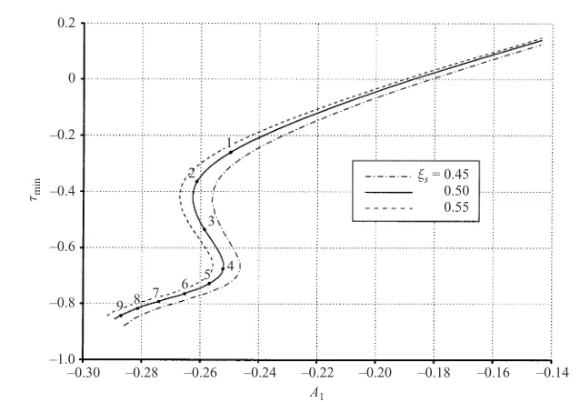
which was found to grow monotonically along the hysteresis curves (see figure 9, §8) representing the family of possible solutions. The calculations were performed with gradually increasing T, and using the solution for previous value of T as an initial guess to solve the problem at T. The corresponding value of the parameter A1 was obtained as a result of the calculation for eachT.
A variable computational star was used for finite-difference representation of
∂ω/∂X3 in the boundary-layer equation (7.2). At the mesh points where the longitu-dinal velocityU was positive,∂ω/∂X3was approximated by a second-order backward difference, otherwise a first-order forward difference was used. To approximate equa-tions (7.1) we used a second-order backward difference for the derivatives with respect tox1for both equations, while the derivative with respect toy1was calculated by using a backward second-order difference for the first equation and a forward second-order difference for the second one.
The main series of calculations was performed on the computational domain
−206x6 20, 0 6y 6 15 with the grid 150×75. We found that as parameter A1 decreases, the size of the separation region grows, and the solution corresponding
C1 L2 A1=−0.24 100×50 0.1182 0.2209
200×100 0.0588 0.1075
A1=−0.29 100×50 0.0980 0.1710 200×100 0.0642 0.0873
Table 1.Comparison of the skin friction inside the interaction region for different meshes.
–0.30 –0.28 –0.26 –0.24 –0.22 –0.20 –0.18 –0.16 –0.14
A1
–1.0 –0.8 –0.6 –0.4 –0.2 0 0.2
τmin
ξs = 0.45
0.50 0.55 1
2
3
4 5 6 7 8 9
Figure 9.Dependence of the minimum skin friction on parameterA1for various shock positions.
for the skin friction using the two norms
C1 = maxX
3 |ω1(X3,0)−ω2(X3,0)| and L2=
"Z X3,max
X3,min
(ω1(X3,0)−ω2(X3,0))2dX3 #1/2
,
and are shown in table 1, which demonstrates apparent convergence of the results as the number of mesh points increases.
8. Numerical results and discussion
–20 –16 –12 –8 –4 0 4 8
X3
–1.0 –0.5 0 0.5 1.5 2.0 2.5
τw
(
X3 ) 1.0
1 2 3 4 5 6 7 8 9
Figure 10.The skin friction distributions for the marked points on the hysteresis curve figure 9.
has three branches. The range ofA1 in which the non-uniqueness is observed proves to depend on the positionξsof the external shock wave. The difference between the three
possible solutions is clearly demonstrated by figure 10. It displays the distribution of the skin friction on the aerofoil surface for a number of selected points on the hysteresis curve (see figure 9). We see that the separation region extends monotonically as the observation point moves along the hysteresis curve. It is interesting to note that the position of the reattachment point remains almost unchanged, while the separation point moves rapidly upstream.
The viscous–inviscid interaction significantly affects the flow behaviour both in the inviscid transonic region 1 and inside the near-wall viscous sublayer 3. For relatively large values of A1 when the separation region only starts to form in the near-wall sublayer, the inviscid transonic flow remains almost unaffected by the boundary layer. For smaller values of A1 when the separation zone increases, its influence on the inviscid flow becomes considerable. A complicated λ-structure of shock waves is observed in the inviscid flow region. The closing primary shock in this structure is due to the global flow pattern on the body scale while the secondary shock that appears some distance upstream results from the interaction process, and is situated just above the point where the flow separation takes place. When A1 becomes even smaller (see figure 11) the flow pattern proves to be more complicated, with two secondary shocks generated by the rather large separation region.
9. Conclusions
–28 –24 –20 –16 –12 –4 0 4 0
2 4 6 8
–8 8
–28 –24 –20 –16 –12 –4 0 4
0 2 4 6 8
–8 8
10 12 14
(b) (a)
Figure 11.The longitudinal velocity isolines in the transonic region (a) and the stream lines in the
viscous sublayer (b) forA1=−0.328.
self-similar solutions provided that the Mach number is close to 1 at the separation point. To study these solutions we introduced a new set of phase variables that allow one to write the governing equations in the form of a non-singular autonomous system. This formulation is significantly more convenient than the one used in the transonic theory starting with Guderley (1957).
We found that the pressure gradient acting upon the boundary layer develops a singularity as the separation point is approached. Being affected by this pressure gradient the fluid inside the boundary layer experiences a sharp deceleration. As a result the slope of the streamline inside the boundary layer increases up to a level where the displacement effect of the boundary layer starts to influence the behaviour of the inviscid flow and the viscous–invicsid interaction region forms.
by comparing figure 10 with the corresponding results, say, in Bodonyi & Smith (1986). Our calculations further show that the solution in the interaction region is non-unique, revealing a hysteresis character of the separating transonic flow.
REFERENCES
Adamson, T. C. & Messiter, A. F.1980 Analysis of two-dimensional interactions between shock
waves and boundary layers.Annu. Rev. Fluid Mech.12, 103–138.
Barish, D. T. & Guderley, G.1953 Asymptotic forms of shock waves in flows over symmetrical
bodies at Mach 1.J. Aeronaut. Sci.13, 491–499.
Bodonyi, R. J.1979 Transonic laminar boundary-layer flow near convex corners.Q. J. Mech. Appl.
Maths 32, 63–71.
Bodonyi, R. J. & Kluwick, A.1977 Freely interacting transonic boundary layers.Phys. Fluids 20,
1432–1437.
Bodonyi, R. J. & Kluwick, A.1982 Supercritical transonic trailing-edge flow. Q. J. Mech. Appl.
Maths 35, 265–277.
Bodonyi, R. J. & Kluwick, A. 1998 Transonic trailing-edge flow. Q. J. Mech. Appl. Maths 51,
297–310.
Bodonyi, R. J. & Smith, F. T.1986 Shock-wave laminar boundary-layer interaction in super-critical
transonic flow.Computers Fluids14, 97–108.
Brilliant, H. M. & Adamson, T. C. 1974 Shock wave boundary-layer interactions in laminar
transonic flow.AIAA J.12, 323–329.
Cole, J. D. & Cook, L. P.1986Transonic Aerodynamics. North-Holland.
Diesperov, V. N. 1980 On one solution of K´arm´an equation describing the flow over a convex
corner.Dokl. Akad. Nauk SSSR254(6), 1367–1371 (in Russian).
Frankl, F. I.1947 Studies in the theory of infinite aspect ration wing moving with the speed of
sound.Dokl. Akad. Nauk SSSR57(7), 1561–1564 (in Russian).
Guderley, G.1957Theorie schallnaher Stro ¨mungen. Springer (Engl. transl.The Theory of Transonic
Flow, Pergamon, 1962).
Korolev, G. L.1987 A method of solving problems in the asymptotic theory of interaction between
the boundary layer and external flow.Zh. Vych. Mat. Mat. Fis.27(8), 1224–1232.
Lagestrom, P. A.1975 Solutions of the Navier–Stokes equations at large Reynolds number.SIAM
J. Appl. Maths28, 202–214.
Messiter, A. F. 1970 Boundary-layer flow near the trailing edge of a flat plate.SIAM J. Appl.
Maths 18, 241–257.
Messiter, A. F.1979 Boundary-layer separation.Proc. 8th US Natl Congr. Appl. Mech., pp. 157–179.
Western Periodicals, North Hollywood, CA.
Messiter, A. F. 1983 Boundary-layer interaction theory. Trans. ASME: J. Appl. Mech. 50 (4b),
1104–1113.
Messiter, A. F., Feo, A. & Melnik, R. E.1971 Shock-wave strength for separation of a laminar
boundary layer at transonic speeds.AIAA J.8(6), 1197–1198.
Murman, E. M. & Cole, J. D.1971 Calculation of plane steady transonic flows.AIAA J.9, 114–121.
Neiland, V. Y.1969 Theory of laminar boundary-layer separation in supersonic flow.Mekh. Zhid.
Gaza(4), 53–57.
Neiland, V. Y.1974 Asymptotic problems in the theory of viscous supersonic flows. Tr. TsAGI
1529.
Neiland, V. Y.1981 Asymptotic theory of boundary-layer separation and interaction with supersonic
gas flows.Usp. Mekh.4(2), 3–62.
Rizzetta, D. P., Burggraf, O. R. & Jenson, R.1978 Triple-deck solutions for viscous supersonic
and hypersonic flow past corners.J. Fluid Mech.89, 535–552.
Ruban, A. I.1974 On laminar separation from a corner point on a solid surface.Uch. Zap. TsAGI
5(2), 44–54.
Ruban, A, I.1978 Numerical solution of the local asymptotic problem of the unsteady separation
of laminar boundary layer in supersonic flow.Zh. Vych. Mat. Mat. Fiz.18(5), 1253–1265.
Rubin, A. I. & Turkyilmaz, I.2000 On laminar separation at a corner point in transonic flow.
Smith, F. T.1982 On the high Reynolds number theory of laminar flows.IMA J. Appl. Maths 28, 207–281.
Stewartson, K.1969 On the flow near the trailing edge of a flat plate II.Mathematika16, 106–121.
Stewartson, K.1974 Multistructured boundary layers on flat plates and related bodies.Adv. Appl.
Mech.14, 145–239.
Stewartson, K.1981 D’Alembert’s paradox.SIAM Rev.23, 308–343.
Stewartson, K. & Williams, P. G.1969 Self-induced separation.Proc. R. Soc. Lond.A312, 181–206.
Sychev, V. V., Ruban, A. I., Sychev, Vic. V. & Korolev, G. L.1998Asymptotic Theory of Separated
Flows. Cambridge University Press.