Scholarship@Western
Scholarship@Western
Electronic Thesis and Dissertation Repository
8-7-2014 12:00 AM
Valuation and Risk Measurement of Guaranteed Annuity Options
Valuation and Risk Measurement of Guaranteed Annuity Options
under Stochastic Environment
under Stochastic Environment
Huan Gao
The University of Western Ontario
Supervisor
Dr. Rogemar Mamon
The University of Western Ontario Joint Supervisor Dr. Xiaoming Liu
The University of Western Ontario
Graduate Program in Statistics and Actuarial Sciences
A thesis submitted in partial fulfillment of the requirements for the degree in Doctor of Philosophy
© Huan Gao 2014
Follow this and additional works at: https://ir.lib.uwo.ca/etd Part of the Other Statistics and Probability Commons
Recommended Citation Recommended Citation
Gao, Huan, "Valuation and Risk Measurement of Guaranteed Annuity Options under Stochastic Environment" (2014). Electronic Thesis and Dissertation Repository. 2257.
https://ir.lib.uwo.ca/etd/2257
This Dissertation/Thesis is brought to you for free and open access by Scholarship@Western. It has been accepted for inclusion in Electronic Thesis and Dissertation Repository by an authorized administrator of
VALUATION AND RISK MEASUREMENT OF GUARANTEED
ANNUITY OPTIONS UNDER STOCHASTIC ENVIRONMENT
(Thesis format: Integrated Article)
by
Huan Gao
Graduate Program in Statistics and Actuarial Science
A thesis submitted in partial fulfillment
of the requirements for the degree of
Ph.D in Statistics
The School of Graduate and Postdoctoral Studies
The University of Western Ontario
London, Ontario, Canada
c
In recent years, there has been a rapid emergence of complex insurance products such as con-tract with option-embedded features. This thesis develops stochastic modelling frameworks for the accurate pricing and risk management of these products. We propose stochastic mod-els for the evolution of the two main risk factors, the interest rate and mortality rate, which could also have a correlation structure. In particular, we focus on the analysis of a guaranteed annuity option (GAO). For the valuation problem, a general framework is put forward where correlated interest and mortality rates are modelled as affine-diffusion processes. A new con-cept of endowment-risk-adjusted measure is introduced to facilitate the calculation of the GAO value. The performance and computational efficiency of the proposed approach are examined through numerical experiments. As a natural offshoot of addressing GAO valuation, we derive the convex-order upper and lower bounds of GAO values by employing the comonotonicity theory. The results via Monte Carlo methodology are used as benchmarks in assessing the accuracy of the comonotonic-based approximated pricing results.
As an alternative to affine structure, we construct a more flexible modelling framework that incorporate regime-switching dynamics of interest and mortality rates in which the switching is governed by a continuous-time Markov chain. Three ways to embed the regime-switching approach to mortality modelling are considered. The corresponding endowment-risk-adjusted measures are constructed and employed to obtain more efficient GAO pricing formulae. An extension of the previous modelling set-up is further developed by integrating the affine struc-ture and regime-switching feastruc-ture. Both interest and mortality risk factors follow a correlated affine structure whilst their volatilities are modulated by a Markov chain process. The change of probability measure technique is again utilised to generate pricing expressions capable of significantly cutting down simulation and computing times.
Finally, the risk management aspect of GAO is investigated by evaluating various risk mea-surement metrics. The bootstrap technique is used to quantify standard error for the estimates of risk measures under a stochastic modelling framework in which death is the only decrement. The moment-based density approximation methods are applied to obtain analytic
tion of the distributions of the loss random variable that provide immediate solutions to the risk measure determination. We also find the relation between the desired accuracy level of risk measures and the required sample size through regression methodology. The sensitivity analyses of risk measures with respect to key parameters are studied demonstrating the utmost importance of reliable estimation and calibration of model parameters.
Keywords: change of probability measure, endowment-risk-adjusted measure, interest rate risk, mortality risk, annuity-contingent derivative, risk measures, regime-switching, Markov chain
I hereby declare that this thesis incorporates materials that are direct results of several related research collaborations. The first two research outputs with my supervisors, Dr. Rogemar Ma-mon and Dr. Xiaoming Liu, have already been published. The remaining research works are manuscripts under review in various peer-reviewed journals or about to be submitted for review.
The content of chapter 2 was used as basis of a full paper (co-authored with Dr. Liu and Dr. Mamon), which was published in Stochastics: (An International Journal of Probability and Stochastic Processes).See reference [34] of chapter 4.
Chapter 3 appeared in theJournal of Computational and Applied Mathematicsas a published paper (co-authored with Dr. Liu and Dr. Mamon); see reference [23] in chapter 2.
A manuscript (co-authored with Dr. Mamon, Dr. Liu and Anton Tenyakov) based on the content of chapter 4 was submitted in December 2013 to the journalInsurance: Mathematics and Economics(IME). Referee’s report was received on 03 June 2014, and the manuscript is currently being revised for resubmission and potential publication in the IME’s Longevity 9 Special Issue in November 2014.
Chapter 5 was already converted to a manuscript (co-authored with Dr. Mamon and Dr. Liu) for submission to theEuropean Actuarial Journal.
The materials in chapter 6 are based on a manuscript (co-authored with Dr. Rogemar Ma-mon and Dr. Xiaoming Liu) that is about to be submitted to theJournal of Risk and Insurance.
Please note that this thesis employed an integrated-article style following Western’s thesis guidelines. This means that each chapter can be read independently as it does not rely on other chapters. Every chapter is therefore deemed to be self-contained and can stand on its own.
With the exception of the guidance on formulating modelling frameworks and occasional help in dealing with numerical experiments from my supervisors, I certify that this document is a product of my own work and efforts.
Acknowledgements
The completion of this work would not have been possible without the support of various indi-viduals who firmly believe in my potential and capability. They kindly offered a lending hand whenever I need help. I, therefore, would like to express my sincere gratitude to my super-visors, instructors, family, and friends who were behind me all the way to reach this level of achievement.
First and foremost, my profound gratefulness goes to my discerning supervisor, Dr. Roge-mar Mamon, for his continual guidance, unflinching support and unfaltering encouragement throughout my entire graduate education. His professionalism, scientific insights and meticu-lous supervision both ensured the accomplishment of this research work and enhanced many transferrable skills, which are priceless for my future career and endeavours. Likewise, I am thankful to my co-supervisor, Dr. Xiaoming Liu, from whom I learnt my first enlightening experience about research. I appreciate her many constructive suggestions over the course of finishing our co-authored papers and this thesis. I am also grateful to the faculty and staffof the Department of Statistical and Actuarial Sciences for their assistance and advice.
Many thanks to my friends who never hesitated to provide their moral support and consola-tion whenever I was in difficulties. The joyful moments spent with them will definitely be part of a lasting happy memory, and their friendship will be cherished forever.
Last but not least, I want to convey my great thanks to my parents for their purest love. With-out their unconditional support and unselfish encouragement, I could not have weathered the hard times, and pursued my dreams, passion and aspirations with utmost persistence. They set themselves as the best example for me to emulate the values of courage, generosity and responsibility. My greatest thanks go to my mother, who is my lifelong mentor. She is full of wisdom and a woman of marked tenacity. My achievements are attributed to her for being the source of my strength and power.
Abstract ii
Co-Authorship Statement iv
Dedication vi
Acknowledgement vii
List of Figures xiii
List of Tables xv
List of Appendices xvii
1 Introduction 1
1.1 Background of stochastic modelling . . . 1
1.2 Research objectives . . . 2
1.2.1 An affine pricing framework for GAO addressing correlated risks . . . . 2
1.2.2 A comonotonicity-based valuation method for GAO . . . 3
1.2.3 The pricing of GAO under a Markov regime-switching framework . . . 3
1.2.4 Valuation of GAO under affine framework with regime-switching volatil-ities . . . 4
1.2.5 Risk measurement of GAO under one-decrement actuarial model frame-work . . . 4
1.3 Review of modelling financial and mortality risks . . . 5
1.3.1 Stochastic modelling of interest rates . . . 5
1.3.2 Stochastic modelling of mortality rates . . . 7
1.3.3 Stochastic modelling in actuarial valuation . . . 8
1.4 Structure of the thesis . . . 10
References . . . 13
2 A generalised pricing framework addressing correlated mortality and interest risks 17 2.1 Introduction . . . 17
2.2 Valuation framework . . . 19
2.2.1 Interest rate model . . . 20
2.2.2 Mortality model . . . 20
2.2.3 Integrated model framework . . . 21
2.2.4 Affine dynamics for mortality and interest risks . . . 22
2.3 The price calculation . . . 23
2.3.1 The forward measure . . . 23
2.3.2 The GAO and its valuation . . . 26
2.3.3 Endowment-risk-adjusted measure for GAOs . . . 27
2.4 Numerical illustration . . . 30
2.5 Conclusions . . . 32
References . . . 36
3 A comonotonicity-based valuation method for guaranteed annuity options 40 3.1 Introduction . . . 40
3.2 The generalised valuation framework . . . 43
3.2.1 The modelling assumptions . . . 43
3.2.2 Valuation formulae obtained via change of num´eraire technique . . . . 47
3.3 Comonotonicity bounds for GAO values . . . 50
3.3.1 Definition of comonotonicity and quantile additivity property . . . 51
3.3.2 Comonotonic upper and lower bounds for the GAO Price . . . 52
3.4 Numerical illustration . . . 56
3.5 Conclusions . . . 58
References . . . 60
4.1 Introduction . . . 66
4.2 Mortality models . . . 70
4.2.1 Model 1 (M1): Gompertz model with BM- and Markov-switching pa-rameters . . . 70
4.2.1.1 Mortality analysis . . . 70
4.2.1.2 Model description . . . 73
4.2.2 Model 2 (M2): Gompertz with pure Markov-switching parameters . . . 80
4.2.3 Model 3 (M3): Regime-switching Luciano-Vigna mortality model . . . 83
4.2.4 Summary of mortality models . . . 84
4.3 Interest rate model . . . 85
4.3.1 Pure Markov interest rate model . . . 86
4.4 Valuation of GAO . . . 87
4.4.1 Pure endowment price . . . 88
4.4.1.1 Pure endowment price under M2 . . . 89
4.4.1.2 Pure endowment price under M3 . . . 89
4.4.2 Endowment-risk-adjusted measure . . . 90
4.4.2.1 GAO price under M2 . . . 90
4.4.2.2 GAO price under M3 . . . 92
4.5 Numerical illustration . . . 94
4.6 Conclusions . . . 96
References . . . 102
5 Pricing a guaranteed annuity option under correlated and regime-switching risk factors 107 5.1 Introduction . . . 107
5.2 Modelling set-up . . . 109
5.3 Derivation of the endowment price . . . 110
5.3.1 Bond price . . . 111
5.3.2 Survival index . . . 112
5.4 GAO valuation . . . 115
5.5 Numerical illustrations . . . 118
5.6 Conclusions . . . 120
References . . . 125
6 Risk measurement of a guaranteed annuity option under a stochastic modelling framework 128 6.1 Introduction . . . 128
6.2 The loss random variable associated with a GAO . . . 131
6.2.1 Description of a GAO contract . . . 131
6.2.2 Modelling framework . . . 132
6.3 Description of risk measures . . . 134
6.3.1 Quantile-based risk measures . . . 134
6.3.2 Distortion risk measures . . . 135
6.3.3 Spectral risk measures . . . 138
6.4 Numerical illustrations . . . 139
6.4.1 Valuation of risk measures . . . 139
6.4.1.1 Monte Carlo method . . . 139
6.4.1.2 Moment-based density approximation . . . 140
6.4.2 Analysis of accuracy . . . 146
6.4.3 Sensitivity analysis . . . 158
6.4.3.1 Impact of interest rate assumptions . . . 158
6.4.3.2 Impact of mortality rate assumptions . . . 158
6.4.3.3 Final remark . . . 160
6.5 Conclusions . . . 160
References . . . 162
7 Concluding remarks 167 7.1 Summary and commentaries . . . 167
7.2 Future research directions . . . 169
References . . . 172
A.2 Derivation of survival probability under M3 . . . 177
Curriculum Vitae 179
List of Figures
3.1 Quantile functions ofS,Sc andSlwithρ=0.9,ρ=0, andρ =−0.9. . . 56
3.2 Relative differences between the approximated quantiles ofSc (orSl) and the simulated quantiles, withρ= 0.9,ρ=0, andρ=−0.9. . . 57
3.3 Contour maps withρ=0.9,ρ=0, andρ= −0.9. . . 57
3.4 The values of the GAO price with its upper and lower approximations. . . 60
4.1 3-dimensional plot of mortality rates versus years and ages. . . 71
4.2 US mortality rate in different years for the period 1933–2009. . . 71
4.3 Evolution of parameters in the Gompertz model based on 1933–2009 US data. . 72
4.4 Contour map of residuals. . . 73
4.5 ξkprocess. . . 75
4.6 Evolution of ˆαunder the 2-state setting. . . 75
4.7 Evolution of ˆβunder the 2-state setting. . . 76
4.8 Evolution of the transition probabilities forξk under the 2-state setting. . . 76
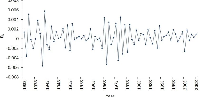
4.9 ηkprocess. . . 78
4.10 Evolution of ˆγunder the 2-state setting. . . 79
4.11 Evolution of ˆζunder the 2-state setting. . . 79
4.12 Evolution of the transition probabilities forηk under the 2-state setting. . . 80
6.1 Histogram approximation. . . 144
6.2 CDF approximation. . . 145
6.3 Risk measures under different samples. . . 149
6.4 Sampling distribution versus bootstrap distribution. . . 150
6.5 Sample size estimate with 5000 as minimum sample size. . . 154
6.6 Sample size estimate with 1000 as minimum sample size. . . 155
6.9 The impact of parameters in the interest rate model on risk measures. . . 159 6.10 The impact of parameters in the mortality rate model on risk measures. . . 159
List of Tables
2.1 Parameter values used in the numerical experiment in chapter 2. . . 32
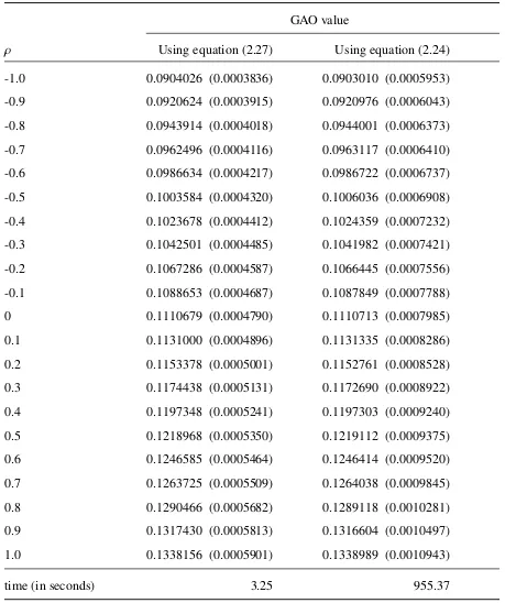
2.2 Actuarial prices for GAO under two different methods in chapter 2. Numbers in parentheses are standard errors. . . 33
3.1 Parameter values used in the numerical experiment in chapter 3. . . 56
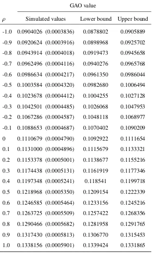
3.2 Actuarial prices for GAO under different methods in chapter 3. Numbers in parentheses are standard errors. . . 59
4.1 Estimated parameters ofξk for different state settings under static calibration. . 77
4.2 Goodness-of-fit test for different models ofξk. . . 78
4.3 Estimated parameters ofηk for different state settings under static calibration. . 81
4.4 Goodness-of-fit test for different models ofηk. . . 81
4.5 Comparison of proposed regime-switching mortality models versus current models. . . 84
4.6 Parameter set for the numerical experiment in regime-switching model frame-work. . . 97
4.7 Actuarial prices for GAO under RSGM (M1). . . 98
4.8 Actuarial prices for GAO under two different methods for M2. . . 99
4.9 Actuarial prices for GAO under two different methods for M3. . . 100
5.1 Parameter set for the numerical experiment in chapter 5. . . 121
5.2 Actuarial prices for GAO under two different methods givenρ= 0.9. . . 122
5.3 Actuarial prices for GAO under two different methods givenρ= 0.5. . . 122
5.4 Actuarial prices for GAO under two different methods givenρ= 0. . . 122
5.5 Actuarial prices for GAO under two different methods givenρ= −0.5. . . 123
mal base densities. . . 143 6.2 Goodness-of-fit (Kolmogorov-Smirnov) test. . . 146 6.3 Parameter values used in the numerical experiment in chapter 6. . . 147 6.4 Risk measures of gross loss for GAO under different sample sizes. Numbers
refer to percentage of the premium. . . 148 6.5 Bootstrap standard error of loss for GAO under different sample sizes
(percent-age). . . 151
List of Appendices
Appendix A Derivation of survival probability in chapter 4 . . . 173
Introduction
1.1
Background of stochastic modelling
Stochastic processes are sequences of random variables indexed with time. They are mathe-matical tools to model and describe time-related random events and phenomena. Stochastic models are utilised widely in the natural sciences, engineering, business and economics; see for instance, Ross [34] and Solberg [35], amongst others. Finance and actuarial science, in particular, have highly benefitted from stochastic methods especially in the valuation of deriva-tives and insurance products, risk management, asset allocation and credit risk analysis.
Insurance valuation and risk management techniques have been traditionally deterministic. But with the recent changes in the investment environments and insurance markets, the important uncertainty element needs to be adequately modelled. For example, many insurance companies have introduced new products with embedded options. These products have similar character-istics to derivatives traded in the financial market. Thus, the pricing of these products requires modern option pricing theory, which inevitably involves the use of stochastic calculus. Due to today’s product sophistication, their value would depend on at least two risk factors, the most important of which are the interest and mortality rates. The risk factors are deemed correlated. Dealing with correlation represents a mathematical as well as a computational hurdle. This is one reason why in previous works, financial and mortality risks are assumed independent.
Chapter1. Introduction 2
Correlation between the two risk factors are nonetheless supported by economic observations. On the one hand, a mortality decline or equivalently an increase in life expectancy can put a huge stress on the country’s social programs and impacts its labour market. This in turn affects local and global economy. An improvement in life expectancy impacts national savings and de-mand on investments, which is directly linked to rate of returns. On the other hand, it is known that interest rate levels directly affect the economy. A high interest rate, for example, implies higher interest payments for debts, which could weaken the capacity of ordinary individuals, especially those saddled with mortgages and borrowings, to afford the much needed medical care and access to advancements in medicine thereby clearly impacting their longevity. It is therefore valid to incorporate the correlation of mortality and interest rates when designing a valuation model. This thesis proposes a stochastic framework to value and manage risks in-volved in guaranteed annuity options (GAOs) by allowing a dependence structure between the two most relevant risk factors.
1.2
Research objectives
To rectify the deficiency of traditional methods in valuation and setting of capital reserve for option-embedded insurance products, we build various stochastic models under which results of theoretical and numerical investigations constitute the contributions of this thesis. The main research objectives are detailed as follows.
1.2.1
An a
ffi
ne pricing framework for GAO addressing correlated risks
and the endowment-risk-adjusted measure, an implementable expression for the GAO price is derived. The development of this model setting, change of measure approach and numerical results are presented in chapter 2. More details about the thesis structure is given in section 1.4.
1.2.2
A comonotonicity-based valuation method for GAO
Following the theme and set-up of the work described in subsection 1.2.1, we offer an alterna-tive method to Monte Carlo simulation in determining the GAO price. As this work involves comonotonicity theory, we deal with the sums of lognormal random variables. Methodolo-gies and approaches in this area were previously developed to find the distribution of sums of lognormal random variables to varying degrees of depth and treatment depending on certain theoretical or practical considerations. Such advances are highlighted in Dufresne [14], Leip-nik [27] and Wu et al. [37]. Our approach is motivated by the works of Dhaene et al. [12, 13], and Liu et al. [28] that proposed the use of comonotonic bounds in approximating the sums of lognormal random variables. Based on the above-mentioned papers, we derive the upper and lower bounds of the price of GAO in convex order together with their quantile functions. Moreover, we investigate the accuracy of our comonotonic bounds by benchmarking them to simulated results generated from the previous work in subsection 1.2.1.
1.2.3
The pricing of GAO under a Markov regime-switching framework
Chapter1. Introduction 4
a continuous- or discrete-time Markov chain. In this work, we continue to apply the concept of endowment-risk-adjusted measure and derive a new transition probability matrix under the new measure. This emphasises the interplay of Girsanov and Bayes theorems.
1.2.4
Valuation of GAO under a
ffi
ne framework with regime-switching
volatilities
The term structure models of interest rates, based on diffusion processes with constant param-eters, may reasonably support the pricing of financial derivatives. However, when we value annuity-linked insurance products which often have long maturities, the constant volatility as-sumption may not be adequate to capture changes in the economy. The same holds true for mortality rates. Therefore, we relax the use of constant volatilities in the stochastic modelling of interest and mortality rates in the affine framework described in section 1.2.1. We assume volatilities of the risk factors evolve according to the dynamics of a continuous-time Markov chain. A modelling framework mixing the affine and correlated structure with the regime-switching feature will be constructed. The valuation process will still be carried out via the change of measure technique but further new results are obtained given the extended frame-work.
1.2.5
Risk measurement of GAO under one-decrement actuarial model
framework
approximation of the loss distribution.
1.3
Review of modelling financial and mortality risks
The purpose of this section is to survey briefly the stochastic modelling of both the interest and mortality rates with a view of employing them to price insurance contracts. We only mention papers that are pertinent to the goals of this thesis as outlined above.
1.3.1
Stochastic modelling of interest rates
The first account of using stochastic processes to model the movement of financial variables can be traced back to the work of Bachelier [1] who used Brownian motion to study the stock and option markets. Since then, stochastic methods were applied to various financial mod-elling endeavors and areas of finance. The field of interest rate theory hugely benefited from the advances made in option pricing theory. Various approaches have been proposed for the modelling of the term structure of interest rates in discrete and continuous time inspired by the pioneering work of Black and Scholes [5] in stock option valuation. The first interest rate model that has considerable impact and continues to permeate financial modelling is the Ornstein-Uhlenbeck-based model for the short rate rt that was put forward by Vasiˇcek [36].
Under any short-rate model, the goal is to calculate the zero-coupon bond price based on the stochastic differential equation that specifies thertprocess. The calculation is performed either
by direct evaluation of the conditional expectation under a risk-neutral measure of a discounted pay-offor by solving a partial differential equation satisfied by the bond price. Cox et al. [11] also proposed an interest rate model based on a Bessel process that ensures positive rates.
As an alternative to the short-rate approach, Heath, Jarrow and Morton (HJM) [23] proposed to model the entire yield curve directly by specifying the dynamics of the forward-rate process. Based on the no-arbitrage conditions of the HJM approach, the implementation only requires the specification of the volatility function.
Chapter1. Introduction 6
developed; see Brigo and Mercurio [7], James and Webber [25], amongst others. As reviewed below, starting in the 1990s, regime-switching term structure models began appearing and have then enriched the short-rate and HJM-type models by the inclusion of hidden Markov chains driving the evolution of parameters.
Elliott & Mamon [16] explored a Markov interest rate model giving a complete characteri-sation of the entire term structure under the assumption that the short rate is a function of a continuous-time Markov chain. In their paper, they proved the well-known Unbiased Expec-tation Hypothesis in economics holds but demonstrated that such relation between the short rate and forward rate holds, provided the expectation must be taken under a forward measure. Their result was employed to obtain an explicit stochastic dynamics for the forward rate. The analytical form of the bond price under the HJM pricing approach was presented as well. Pi-oneering works to model economic variables as a regime-switching process can be found in Hamilton [21]. Contributions from many authors to short-rate modelling then ensued. In these contributions, the parameters are ensured to change over time and controlled by a Markov state variable. Bekaert et al. [4], Evans and Lewis [19], Garcia and Perron [20] conducted empirical studies to test the validity of regime switches in interest rates.
1.3.2
Stochastic modelling of mortality rates
Pricing calculations in life insurance contracts and pension plans make use of a mortality as-sumption, commonly described as the annual probabilities of death rate or the force of mortal-ity. In a traditional framework, these quantities are obtained using observed data. Given the future uncertainty on mortality levels due to medical breakthroughs and discoveries in phar-macology as well as the creation of insurance products with derivative features, researchers began giving attention to stochastic mortality models that are also compatible and consistent with stochastic models used in the pricing of financial products.
The beginning of stochastic modelling of mortality can be attributed to Lee and Carter (LC) [26] who proposed to model central death rates representing age-specific mortality. An essen-tial ingredient of their method is a univariate mortality index that describes the variation of mortality patterns over time. Due to the absence of observable variable in their model, mak-ing traditional regression method invalid, smak-ingular-value decomposition was employed in their parameter estimation. A one-parameter life table was constructed and fitted to US mortality patterns. Forecasts of rates and life expectancy were obtained under the assumption that future trends would continue in the same way. The key feature of the LC methodology is that it gives allowance to uncertainty in mortality rate by modelling it as a stochastic process. Subsequent research works on stochastic mortality were built upon LC’s methodology. Brouhns et al. [8] made some improvements to the LC model by using a Poisson random variation for the num-ber of deaths instead of the additive error term in the original model. This is deemed more reasonable since the mortality rate is much more variable at older ages than at younger ages.
Chapter1. Introduction 8
the other one affects mortality rate dynamics at higher ages much more than at lower ages. Empirical evidence supports that both factors are necessary to achieve a satisfactory fit over the entire mortality term structure. One important advantage of their method is that it allows different improvements at different ages and at different times which can not be achieved in LC model.
In 2005, Luciano and Vigna [29] adopted affine processes to describe the evolution of mortality rate and provided detailed calibration using UK data. In their paper, they suggested that a non-mean-reverting process is more suitable to model mortality rate than a non-mean-reverting one. On the other hand, the addition of negative jumps into the diffusion process performed better to fit the real mortality data and forecast the mortality trend.
Research advances in modern finance have stimulated research developments in the field of in-surance. Milidonis et al. [32] brought the concept of regime-switching approach into mortality rate modelling. In their paper, the advantages of applying regime-switching models into mor-tality rate modelling were highlighted. Through the investigation of the US population mortal-ity index, they illustrated that there were structural changes in the underlying death probabilmortal-ity for all age cohorts from all death causes, which provided evidence in the adoption of regime-switching models. Moreover, they applied the concept of regime-regime-switching to model the error term of mortality index in the LC model. This captures the disturbances introduced by extreme observations over time and makes the error term non-normal.
1.3.3
Stochastic modelling in actuarial valuation
measure technique assuming a swaption hedge. Ballotta and Haberman [3] examined the val-uation of annuity-contingent options and extended the research results in Ballotta and Haber-man [2], which assumed unsystematic mortality risk; they introduced an integrated framework to value GAO using option pricing methodology of modern finance. In their frameworks, a stochastic model for the evolution of mortality rate was considered whilst the term structure of interest rate evolves according to a single-factor HJM model. A fair value for GAO was derived through the change of measure technique. To make the estimation of the value of GAO implementable, Monte-Carlo simulation technique was applied. Moreover, the sensitivity of GAO prices with respect to key parameters was investigated. However, whilst the two types of risks are stochastic in their valuation, they are still assumed independent.
In Chu and Kwok [10], three analytical approximation methods were proposed for GAO pric-ing, namely, the stochastic duration approach, Edgeworth expansion and multi-factor affine interest rate model setting. The stochastic duration approach is based on the minimisation of the price error whilst the Edgeworth expansion method approximates the probability distribu-tion of the annuity value at maturity of the contract. For the affine approximation, the concave exercise boundary is approximated by a hyperplane in order to obtain the exercise probabil-ity of the annuprobabil-ity option. The three analytic approximation methods were compared in terms of both numerical accuracy and computational efficiency and a sensitivity of GAO prices was performed.
Jalen and Mamon [24] proposed an integrated framework of stochastic mortality and interest rates to price insurance claims. They relaxed the independence assumption of the two risk fac-tors. In their framework, the mortality rate was modelled as an affine-type diffusion process just like the short rate process. Through the change of measure technique, analytical expressions in mortality-linked insurance products were presented. Their approach provided new perspec-tives and methodology in the valuation of other insurance products under a more reasonable assumption that risk factors are dependent.
con-Chapter1. Introduction 10
ditional expected present value random variable of the annuity’s future payments. The two risk factors were modelled as stochastic processes; the mortality rate followed the LC model and the short rate followed the Vasiˇcek model. They applied the concept and properties of comonotonicity in the derivation of the convex-order lower and upper order of the annuity rate. The accuracy of the bounds was validated through numerical analysis. This approach has the advantage of mathematical tractability in computing the distribution function for the sum of comonotonic random variables, which could be adopted in the further calculation of other annuity-linked products.
The valuation of a related product, called guaranteed lifelong withdrawal benefit options with variable annuity, was described by Piscopo and Haberman [33]. In their paper, the equity risk followed the geometric Brownian motion whilst the mortality rate was based on the standard mortality tables with allowance for the possible perturbations having a regime-switching fea-ture. They provided the fair value through Monte Carlo simulations under different scenarios and conducted sensitivity analysis to show the relation between the variation of parameters and the value of the product.
1.4
Structure of the thesis
This thesis consists of 7 chapters. The succeeding chapters are the compilation of related re-search papers (2 published, 1 under review and 2 for submission) on the valuation and risk measurement of GAOs with the stochastic modelling of risk factors.
Chapter 3 presents an alternative way to value GAO under the model framework in chapter 2. Comonotonicity theory is applied to derive upper and lower bounds for the annuity rate in the convex order sense. These bounds provide accurate approximations for the value of GAOs. Numerical illustrations are included to show the accuracy and practical applicability of our comonotonic approximations for the GAO values benchmarked by simulated results in chapter 2.
In chapter 4, we consider three ways of developing a regime-switching approach in modelling the evolution of mortality rates for the purpose of pricing a GAO. This involves the extension of the Gompertz and non-mean reverting models as well as the adoption of a pure Markov model for the force of mortality. A continuous-time finite-state Markov chain is employed to describe the evolution of mortality model parameters which are then estimated using the filtered-based and least-squares methods. The adequacy of the regime-switching Gompertz model for the US mortality data is demonstrated via the goodness-of-fit metrics and likelihood-based selection criteria. A GAO is valued assuming the interest and mortality risk factors are switching regimes in accordance with the dynamics of two independent Markov chains. To obtain closed-form valuation formulae, we employ the change of measure technique with the pure endowment price as the num´eraire. Numerical implementations are included to compare the results of the proposed approaches and those from the Monte Carlo simulations.
An extended modelling framework building from that in chapter 2 is proposed in chapter 5. The volatilities of the interest rate and mortality rate are regime-switching driven by a finite-state continuous time Markov chain. We derive the explicit solution to the endowment price which involves solving the linear system of ordinary differential equations by employing the forward measure. Utilising the endowment-risk-adjusted measure with endowment as the num´eraire, we provide an efficient formula for GAO price as supported by numerical experiments produc-ing results that have smaller errors and with less computproduc-ing time.
Chapter1. Introduction 12
for the gross loss random variable is developed. We consider a one-decrement actuarial model for the gross loss in which death is the only decrement, and the financial and mortality risk factors follow correlated affine structures. Risk measures are determined using the moment-based density method and benchmarked with the Monte-Carlo simulation method. A bootstrap technique is utilised to assess the variability of risk measure estimates. We establish the re-lation between the level of desired risk measure accuracy and required sample size under the constraints of computing time and memory. A test of GAO sensitivity to model parameters demonstrates the need for accurate model estimation and calibration. Our numerical investiga-tions should prove useful to insurers in adhering to certain regulatory requirements.
[1] Bachelier, L. (1990), “Theory of speculation,”Annales scientifiques de l’Ecole Normale Superieure, 17, 21–86.
[2] Ballotta, L. and Haberman, S. (2003), “Valuation of guaranteed annuity conversion op-tions,”Insurance: Mathematics and Economics, 33, 87–108.
[3] Ballotta, L. and Haberman, S. (2006), “The fair valuation problem of guaranteed annuity options: the stochastic mortality environment case,”Insurance: Mathematics and Eco-nomics, 38, 195–214.
[4] Bekaert, G., Hodrick, R. and Marshall, D. (2001), “Peso problem explanations for term structure anomalies,”Journal of Financial Economics, 48, 241–270.
[5] Black, F. and Scholes, M. (1973), “The pricing of options and corporate liabilities,” Jour-nal of Political Economy, 81, 637–659.
[6] Boyle, P. and Hardy, M. (2003), “Guaranteed annuity options,” ASTIN Bulletin, 33(2), 125–152.
[7] Brigo, D. and Mercurio, F. (2006), Interest Rate Models – Theory and Practice: With Smile, Inflation and Credit, Springer Finance, Berlin.
[8] Brouhns, N., Denuit, M. and Vermunt, J. (2002), “A Poisson log-bilinear approach to the construction of projected lifetables,” Insurance: Mathematics and Economics, 31, 373–393.
[9] Cairns, A., Blake, D. and Dowd, K. (2006), “Pricing death: frameworks for the valuation and securitization of mortality risk,”ASTIN Bulletin, 36, 79–120.
REFERENCES 14
[10] Chu, C. and Kwok, Y. (2007), “Valuation of guaranteed annuity options in affine term and structure models,” International Journal of Theoretical and Applied Finance, 10, 363–387.
[11] Cox, J., Ingersoll, J. and Ross, S. (1985), “A theory of the term structure of interest rates,” Econometrica, 53, 385–407.
[12] Dhaene, J., Denuit, M., Goovaerts, M., Kaas, R. and Vyncke, D. (2002a), “The concept of comonotonicity in actuarial science and finance: theory,”Insurance: Mathematics and Economics, 31, 3–33.
[13] Dhaene, J., Denuit, M., Goovaerts, M., Kaas, R. and Vyncke, D. (2002b), “The concept of comonotonicity in actuarial science and finance: applications,”Insurance: Mathematics and Economics, 31, 133–161.
[14] Dufresne, D. (2004), “The log-normal approximation in financial and other applications,” Advances and Applications of Probability, 36, 747–773.
[15] Elliott, R. and Mamon, R. (2002), “An interest rate model with a Markovian mean revert-ing level,”Quantitative Finance, 2, 454–458.
[16] Elliott, R. and Mamon, R. (2003), “A complete yield curve description of a Markov inter-est rate model,”International Journal of Theoretical and Applied Finance, 6, 317–326. [17] Elliott, R., Siu, T. and Chan, L. (2007), “Pricing volatility swaps under Heston’s stochastic
volatility model with regime switching,”Applied Mathematical Finance, 14, 41–62. [18] Elliott, R. and Siu, T. (2009), “On Markov-modulated exponential-affine bond price
for-mulae,”Applied Mathematical Finance, 16, 1–15.
[19] Evans, M. and Lewis, K. (1994), “Do expected shifts in inflation affect estimates of the long-run Fisher relation?”Journal of Finance, 50, 225–253.
[21] Hamiton, J. (1989), “A new approach to the economics analysis of nonstationary time series and the business cycle,”Econometrica, 57, 357–384.
[22] Hardy, M. (2003), Investment Guarantees: Modeling and Risk Management for Equity-Linked Life Insurance, Wiley & Sons, New Jersey.
[23] Heath, D., Jarrow, R. and Morton, A. (1992), “Bond pricing and the term structure of interest rates: a new methodology for contingent claims valuation,” Econometrica, 60, 77–105.
[24] Jalen, L. and Mamon, R. (2009), “Valuation of contingent claims with mortality and interest rate risks,”Mathematical and Computer Modelling, 49, 1893–1904.
[25] James, J. and Webber, N. (2000),Interest Rate Modelling, Wiley, New York.
[26] Lee, R. and Carter, L. (1992), “Modeling and forecasting US mortality,” Journal of the American Statistical Association, 87, 659–675.
[27] Leipnik, R. (1991), “On lognormal normal random variables: the characteristic function,” Journal of the Australian Mathematical Society: Series B, 32, 327–347.
[28] Liu, X., Jang, J. and Kim, S. (2011), “An application of comonotonicity theory in a stochastic life annuity framework,” Insurance: Mathematics and Economics, 48, 271– 279.
[29] Luciano, E. and Vigna, E. (2005), “Non mean reverting affine processes for stochastic mortality,”Carlo Alberto Notebook 30/06 and ICER WP 4/05.
[30] Mamon, R. and Elliott, R. (2007),Hidden Markov Models in Finance,International Series in Operations Research & Management Science, Volume 104, Springer, New York. [31] Mamon, R. and Elliott, R. (2014), Hidden Markov Models in Finance: Further
Devel-opments and Applications,International Series in Operations Research & Management Science, Volume 209, Springer, New York.
REFERENCES 16
[33] Piscopo, G. and Haberman, S. (2012), “The valuation of guaranteed lifelong withdrawal benefit options in variable annuity contracts and the impact of mortality risk,” North American Actuarial Journal, 15(1), 59–76.
[34] Ross, S. (2010),Introduction to Probability Models,10th edition, Academic Press, Mas-sachusetts.
[35] Solberg, J. (2009),Modeling Random Processes for Engineers and Managers, John Wiley & Sons, New Jersey.
[36] Vasiˇcek, O. (1977), “An equilibrium characterisation of the term structure,” Journal of Financial Economics, 5(2), 177–188.
A generalised pricing framework
addressing correlated mortality and
interest risks
2.1
Introduction
It is a well-accepted fact that annuity products are notably influenced by both interest and mortality risks. However, the methodology for dealing with these two risks is fundamentally oversimplified under the traditional actuarial approach. Mortality risk is usually regarded as secondary in importance compared to the volatile nature of interest risk. In addition, mortality risk is deemed diversifiable if the insurer holds a sufficiently large portfolio of similar con-tracts. As a result, mortality is traditionally modelled deterministically, whilst interest risk is modelled stochastically. Modern finance theory is then adopted for pricing and risk analysing annuity-related insurance products; see for example, Ballotta and Haberman [1], Boyle and Hardy [7], Lin and Tan [20], amongst others. Apparently, the deterministic modelling of mor-tality rates has the advantage that it makes the valuation problem more manageable since this implies mortality risk is independent from interest rate risk. Nonetheless, such framework as-suming independence between the primary risk factors is too simplistic.
Chapter2. Ageneralised pricing framework addressing correlated mortality and interest risks18
The perspective of deterministic mortality has been challenged in the last few years. It has been observed that recent mortality trends show some unprecedented improvement along with a great deal of uncertainty. The insurance industry as well as pension fund companies are thus exposed to substantial systematic mortality risk. Insurers underestimated the significance of mortality risk which led to emerging insolvency issues for many insurance companies that sold guaranteed annuity options (GAOs) between the late 70s and 80s. It caused the closure to new business in 2000 of Equitable Life, one of oldest life insurance companies in the UK. This in-surance mishap has stimulated discussions on mortality/longevity risk and has since called for stochastic approach for mortality modelling; see Pitacco [30, 31] and the references therein. Biffis [3] explored the parallelism between interest and mortality rates and proposed affine-type stochastic models for mortality dynamics. In Luciano and Vigna [25], an empirical study found that non-mean reverting OU process fits the historical data better than the mean-reverting pro-cess.
Nonetheless, the majority of the aforementioned papers concerning this problem do not prop-erly treat the correlation between interest and mortality rates; in particular, only one factor is considered stochastic and the other remaining factor is assumed deterministic. This work presents a generalised set-up and approach under which the pricing solution is obtained with great ease despite dependence between two stochastic factors. We demonstrate how to use the change of measure technique in the pricing of an annuity-linked option. More specifically, a new measure associated with the pure endowment as num´eraire is constructed to solve the GAO pricing problem. We note that Dahl et al. [11] also utilised the change of measure tech-nique to facilitate the pricing of survivor swaps. Nevertheless, whilst the likelihood process is constructed, the associated num´eraire with the measure change is not categorically identified. In this work, we lay down the groundwork to get a simplified expression for the conditional expectation under the risk-neutral measure. By popularising this technique, which is not com-monly used in actuarial science and insurance, it is hoped that its power and utility can be fully explored for other contingent claim valuation problems.
The formulation of the pricing framework is presented in section 2.2; in particular, this sec-tion outlines the assumpsec-tions for the models of interest and mortality rate processes and their dependence. An integrated set-up is also developed. In section 2.3, we describe the change of probability measure approach to aid the evaluation of conditional expectation necessary to determine the value of a GAO. The forward measure is revisited and the pure endowment-risk-adjusted measure is defined. Section 2.4 presents a numerical example illustrating the applicability and benefits of our proposed approach. Finally, in section 2.5, we provide some concluding remarks and further directions.
2.2
Valuation framework
Chapter2. Ageneralised pricing framework addressing correlated mortality and interest risks20
support to insurance and pension business, a coherent and integrated modelling framework is necessary. We present in this section a brief theoretical background and considerations on risk-neutral modelling of risk factors. A comprehensive discussion can be found in Biffis [3] and Cairns et al. [8]. We give general descriptions for each interest rate process and mortality rate process, and then form a combined modelling set-up. An important aspect of any valuation model or modelling approach is the balance between complexity and computational tractability of both pricing and parameter estimation. In the last subsection, we assume that both interest rate and mortality rate dynamics are modulated by affine processes. This implies that we are able to exploit the analytical tractability of these processes within the context of reflecting both factors into the valuation approach.
2.2.1
Interest rate model
The modern approach to valuation of bonds and interest rate derivatives employs martingale theory to obtain no-arbitrage price and hedging strategies. To value a contingent claim, we need the risk-free cash accountBt which is governed by the differential equation
dBt = rtBtdt, or equivalently Bt = B0e
Rt
0rudu.
The processrt is called the continuously compounded rate of interest for a riskless investment.
We assume that a risk-neutral measure or the so-called martingale measure, Q, exists. Under Q, the discounted price of a risky asset is a martingale using B−1
t as the discount factor or Bt
as the num´eraire. Thus, the bond price at timetfor a zero-coupon bond paying $1 at maturity T >tis given by
B(t,T)= EQ
e−
RT t rudu
Rt
,
whereRt is the filtration generated by thert process.
2.2.2
Mortality model
with age x+t. Write
S(t,x) :=e−
Rt
0µ(s,x+s)ds. (2.1)
Under the assumption of deterministic mortality,S(t,x) is the survival probability for a person currently aged xsurviving for the next t years. Under the stochastic approach, however, this survival probabilityS(t,x) itself becomes a random variable, and its value can only be observed at time t rather than at time 0. For the purpose of pricing, we need to calculate the expected value of the random variableS(t,x). Thus,
P(0,t,x) : = E[I{τ≥t}|M0]=E
S(t,x)
M0 = E e− Rt
0µ(s,x+s)ds
M0 , (2.2)
whereIis an indicator function. Furthermore,
P(t,T,x) : = E[I{τ≥T}|Mt]=I{τ≥t}E
"
S(T,x) S(t,x)
Mt #
= I{τ≥t}E
e−
RT
t µ(s,x+s)ds
Mt (2.3)
= I{τ≥t}P(t,T,x). (2.4)
The distinction between P(0,t,x) and P(t,T,x) given in equations (2.2) and (2.4) must be noted. Throughout the entire chapter, we employ the bold font to refer to the function that is conditional on survival up to timet, otherwise the regular font is used. We call P(t,T,x) :=
E
e−
RT
t µ(s,x+s)ds
Mt
thesurvival functionunder the associated measure where the expectation is taken. When it is calculated under the real measure,P(t,T,x) can be interpreted as thecentral predicted survival function. When it is calculated under the risk-neutral measure, P(t,T,x) can be interpreted asrisk-adjusted survival functionto account for the adverse selection or to reflect the risk-premium adjustment on behalf of the insurance companies. In the succeeding discussion, we shall omit the reference to age xin the survival function and simply write it as P(t,T).
2.2.3
Integrated model framework
We define the filtrationFt asFt := Rt ∨ Mt = σ(Rt ∪ Mt), which refers to the joint filtration
Chapter2. Ageneralised pricing framework addressing correlated mortality and interest risks22
survival benefit using no-arbitrage theory, with both interest and mortality rate being stochastic. For instance, let M(t,T;x) = M(t,T) be the fair value of a survival benefit of $1 payable at time T for a life aged x at time t < T. From the risk-neutral pricing principle, we have the survival benefit value given by
M(t,T)= EQ
e−
RT
t rudu ·I{τ≥T}
Ft
=I{τ≥t}·EQ
e−
RT t rudue−
RT t µvdv
Ft . (2.5) For a general payofffunctionCT conditional on the survival at timeT, the value ofCt can be
obtained as follows:
Ct =EQ
e−
RT
t rudu ·I{τ≥T}·CT
Ft
= I{τ≥t}·EQ
e−
RT t rudue−
RT
t µvdv·CT
Ft . (2.6)
Remark: The use of bold M and C in equations(2.5) and(2.6), respectively, emphasises the conditioning on survival through the indicator function. In particular,
M(t,T)= I{τ≥t}M(t,T), and Ct = I{τ≥t}Ct.
2.2.4
A
ffi
ne dynamics for mortality and interest risks
We assume that under a filtered probability space (Ω,F,{Ft},Q), where Q is a risk-neutral
measure, the respective dynamics of the interest rate processrt and force of mortalityµt for an
insured aged xat time 0 are given by
drt =a(b−rt)dt+σdWt1 (2.7)
and
dµt = cµtdt+ξdZt, (2.8)
where a, b, c, σ and ξ are positive constants, and Zt = ρWt1 +
p
1−ρ2W2
t. Here, Wt1 and
Wt2 are independent standard Brownian motions. This means that Zt in equation (2.8) is also
a Brownian motion correlated with Wt1. Both the initial valuesr0 and µ0 are assumed to be known at time 0.
drawback that theoretically it is possible to generate negative interest or mortality rates. The issue of negative interest rates has been widely discussed in the literature; this problem can be mitigated by appropriately choosing model parameter values or using the extended Vasiˇcek model, i.e. the Hull and White model [cf. page 45 of Pelsser [29]]. The use of mortality model in (2.8) was justified by Luciano and Vigna [26] [cf. page 8], showing that the proba-bility of negative mortality rates is negligible with the calibrated parameters. These particular interest and mortality rate models are employed in this work due to their tractability. They clearly facilitate the application of the change-of-measure approach in the evaluation of the risk-neutral conditional expectation for purpose of valuation, similar to the canonical example of Black-Scholes model in option pricing. Analytic expressions for the dynamics of the two underlying risk factors under the new measure can be derived under this modelling set-up, lead-ing to a more implementable formula for the valuation of guaranteed annuity options (GAOs), as demonstrated in section 2.3.
The priceB(t,T) of aT−maturity zero-coupon bond at timet <T is known to be given by B(t,T)= EQ
e−
RT t rudu
Ft
= e−A(t,T)rt+D(t,T), (2.9) where
A(t,T) = 1−e
−a(T−t)
a and (2.10)
D(t,T) = b− σ
2 2a2
!
[A(t,T)−(T −t)]− σ
2A(t,T)2
4a . (2.11)
See Bj¨ork [5] or Mamon [27] for details of the result in (2.9).
2.3
The price calculation
2.3.1
The forward measure
Chapter2. Ageneralised pricing framework addressing correlated mortality and interest risks24
market account Bt as the num´eraire. Now, we could also choose the bond price B(t,T) as a
num´eraire. Associated with B(t,T), we define the forward measure Qeequivalent to the
risk-neutral measureQvia the Radon-Nikodˆym derivativeΛT by setting
dQe
dQ F T
= ΛT :=
e−
RT
0 ruduB(T,T)
B(0,T) . (2.12)
Note thatB(T,T)=1 in equation (2.12). Under measureQ,ΛT is a martingale, and fort≤ T,
Λt =EQ[ΛT|Ft]=
e−
Rt
0ruduB(t,T)
B(0,T) .
From Bayes’ rule, we know that for anyFt−measurable random variableH,
EQe
[H|Ft]=
EQ[Λ TH|Ft]
EQ[Λ T|Ft]
, (2.13)
which implies that
EQe
[H|Ft]=
EQe−RT
t ruduH
Ft
B(t,T) . Or equivalently,
EQ
e−
RT t ruduH
Ft
= B(t,T)EQe
[H|Ft]. (2.14)
Thus, equation (2.5) can be expressed as
M(t,T) = B(t,T)EQeh
I{τ≥T}
Ft
i
(2.15)
= I{τ≥t}B(t,T)EQe
e−
RT t µvdv
Ft . (2.16)
We note that the term EQe
e−
RT t µvdv
Ft
:= P(t,T) in equation (2.16) is the survival function underQe.Therefore, if we have the dynamics ofµtunderQethen the explicit solution forP(t,T)
follows.
Following the result given and established in Appendix of Mamon [27], we have
whereWet1andWet2are standard Brownian motions underQ, and the functione A(t,T) is specified
in equation (2.10). Hence, the respective dynamics under Qe of rt and µt are given by the
stochastic differential equations (SDEs) drt =
h
ab−σ2A(t,T)−art
i
dt+σdWet1 (2.17)
and
dµt = cµtdt+ρξdWt1+
p
1−ρ2ξdW2
t
= (−ρσξA(t,T)+cµt)dt+ρξdWet1+ p
1−ρ2ξd
e
Wt2
= (−ρσξA(t,T)+cµt)dt+ξdZet, (2.18)
whereeZt = ρWet1 + p
1−ρ2
e
Wt2. From equation (2.18), we see thatµt has an affine form with
time-dependent drift. Note that, if there is no correlation between the processesrt andµt, i.e.
ρ =0, the dynamics ofµt does not change under the forward measureQ. Formula (2.16) thene
reduces to the case whenrtandµt are independent.
Writeα(t) := −ρσξA(t,T) andb(t) :=
Z t
0
(−c)du =−ct.Then
µt =e
−b(t) µ 0+
Z t
0
eb(v)α(v)dv+eb(v)ξdeZv
!
.
By letting
γ(t)=
Z T
t
e−b(v)dv = e
cT −
ect
c =
ect c (e
c(T−t)− 1) and employing the result in pp. 267-268 of Elliott and Kopp [15], we have
P(t,T) = EQe
e−
RT t µvdv
Ft
= EQe
e−
RT t µvdv
µt
by the Markov property
= e−µtGe(t,T)+He(t,T),
(2.19) where
e
G(t,T)=eb(t)
Z T t
e−b(u)du = eb(t)γ(t)= (e
c(T−t)−1)
c (2.20)
and
e
H(t,T) = −
Z T
t
eb(u)α(u)γ(u)− 1
2e
2b(u)ξ2(u)γ2(u)
! du = ρσξ ac − ξ2 2c2 !
[G(te ,T)−(T −t)]+
ρσξ
ac [A(t,T)−φ(t,T)]+
ξ2
4cG(te ,T) 2
Chapter2. Ageneralised pricing framework addressing correlated mortality and interest risks26
withφ(t,T)= 1−e−a(a−−cc)(T−t) .
Combining equations (2.9)–(2.11), (2.16), and (2.19)–(2.21), we have M(t,T) = e−(A(t,T)rt+Ge(t,T)µt)+D(t,T)+He(t,T)
= β(t,T)e−V(t,T), (2.22) whereβ(t,T)= eD(t,T)+He(t,T)
andV(t,T)= A(t,T)rt+G(te ,T)µt.
2.3.2
The GAO and its valuation
We now consider the GAO valuation problem. A GAO can be viewed as a contract that gives the policyholder the right to convert the survival benefit into an annuity at a pre-specified con-version rate. This type of option first gained popularity in UK pension policies during the late 70s and 80s. Since then it became a common feature of policies sold in many countries.
The guaranteed conversion rate, g, can be quoted as an annuity/cash value ratio. According to Bolton et al. [6], the most commonly used guaranteed rate for males, aged 65 in UK in the 80s, was g = 19, meaning that a £1000 cash value can be turned into an annuity of £111 per annum. If the guaranteed conversion rate is higher than the prevailing conversion rate, the GAO is of positive value; otherwise, the GAO is valueless since the policyholder could use the cash to obtain higher value of annuity from the primary market. Therefore, the moneyness of the GAO at maturity depends on the price of annuity available from the primary market at that time, which are determined by the prevailing interest and mortality rates.
Letax(T) be the prevailing annuity rate in the primary market. Since the annuity payments can
be considered as a sequence of survival benefit $1 at the beginning of each year, we can use equation (2.22) to get
ax(T) =
∞
X
n=0
EQ
e−
RT+n T rudue−
RT+n T µvdv
FT
= ∞
X
n=0
M(T,T +n)=
∞
X
n=0
whereβ(T,T +n)= eD(T,T+n)+He(T,T+n)
andV(T,T +n)=A(T,T +n)rT +G(Te ,T +n)µT.
Then the payofffunction of the GAO at timeT, based on each one dollar cash amount, is
CT =I{τ≥T}[g·ax(T)−1]+ =gI{τ≥T}
"
ax(T)−
1 g
#+
.
Our valuation problem is to determine the price of GAO at time 0, which is
PGAO = EQ
e−
RT
0 ruduCT
F0
= gEQ
e−
RT
0 rudue−
RT
0 µvdv(a
x(T)−K)+
F0 , (2.24)
whereax(T) is defined in equation (2.23) andK is 1/g.
In the next subsection, we employ a change of num´eraire technique to evaluate equation (2.24) straightforwardly despite the dependence betweenrtandµt, and the complicated form ofax(T).
We invoke the idea of change of probability measures in order to explicitly price contingent claims; see Dahl et al. [11] and Jalen and Mamon [16]. We then show how to derive the dynamicsµt andrt under this new measure that will facilitate the GAO price calculation.
2.3.3
Endowment-risk-adjusted measure for GAOs
We introduce a new measure associated with the pure endowment M(t,T) as the num´eraire. The new measure is then called the endowment-risk-adjusted measureQb. The measure is
de-fined via the Radon-Nikodˆym derivative dQb
dQ :=ηT = e−
RT
0 ruduM(T,T)
M(0,T) . (2.25)
Note that M(T,T)=I{τ≥T} in equation (2.25). SinceηT is a martingale, then fort ≤T,
ηt =EQ[ηT|Ft]=
e−
Rt
0ruduM(t,T)
M(0,T) . (2.26)
UtilisingQ, equation (2.24) can be re-written asb
PGAO = gEQ
e−
RT
0 rudue−
RT
0 µvdv
F0
EQbh
(ax(T)−K)+
F0
Chapter2. Ageneralised pricing framework addressing correlated mortality and interest risks28
based on the similar Bayes’ rule argument following equation (2.13).
From equations (2.5), (2.23) and (2.24), we have
PGAO = g M(0,T)EQb
h
(ax(T)−K)+
F0
i
= g M(0,T)EQb
∞ X
n=0
β(T,T +n)e−V(T,T+n)−K
+ F0
. (2.27)
To evaluate equation (2.27), we need the dynamics under Qbof the mortality and interest rate
processes. We consider the dynamics ofe−
Rt
0ruduM(t,T)=e−
Rt
0ruduB(t,T)P(t,T) := Xtin (2.26).
Suppose X1
t := e
−Rt
0ruduB(t,T) and X2
t := P(t,T). We are interested to find dXt where Xt =
Xt1Xt2.
From equations (2.9) and (2.7), one may verify that
dX1t = −σA(t,T)X
1
tdW
1
t. (2.28)
LetY(t) :=−G(te ,T)µt+H(te ,T) in equation (2.19), i.e.,X2t := P(t,T)=eY(t). Then we have
dY(t)=
∂H(te ,T)
∂t −
∂G(te ,T)
∂t µt−cµtG(te ,T)
dt−ξG(te ,T)dZt
and therefore
dX2t = 1 2e
Y(t)ξ
e
G(t,T)2dt+eY(t)dY(t)
= eY(t)
1 2
ξG(te ,T) 2 dt+
∂H(te ,T)
∂t −
∂G(te ,T)
∂t +cG(te ,T)
µt
dt−ξG(te ,T)dZt
= Xt2
∂H(te ,T)
∂t + 1
2(ξG(te ,T)) 2−
∂G(te ,T)
∂t +cG(te ,T)
µt
dt−ξG(te ,T)dZt
,(2.29)
wheredZt =ρdWt1+
p
1−ρ2dW2
SinceXt = Xt1Xt2,we have
dXt = Xt1dX
2
t +X
2
tdX
1
t +
−Xt1σA(t,T) −X
2
tξG(te ,T)
ρdt
= Xt1X
2
t
∂H(te ,T)
∂t + 1
2(ξG(te ,T)) 2−
∂G(te ,T)
∂t +cG(te ,T)
µtdt−ξG(te ,T)dZt
−σA(t,T)dWt1+ρσξA(t,T)G(te ,T)dt !
= Xt
∂H(te ,T)
∂t +ρσξA(t,T)G(te ,T)+ 1
2(ξG(te ,T)) 2−
∂G(te ,T)
∂t +cG(te ,T)
µt
dt
+Xt
h
−σA(t,T)dWt1−ξG(te ,T)(ρdWt1+ p
1−ρ2dW2
t)
i
. (2.30)
Note that thedtterm of equation (2.30) must be identically zero sinceX(t)= e−
Rt
0ruduM(t,T) is
a martingale process (being a discounted process) underQ.That is, dXt
Xt
=−σA(t,T)dWt1+ξG(te ,T)(ρdWt1+ p
1−ρ2dW2
t)
. (2.31)
Utilising equation (2.31), we find that d(lnXt) =
1 Xt
dXt−
1 2
1 (Xt)2
(dXt)2
=
"
−1
2
σA(t,T)+ρξG(te ,T) 2
− 1
2(1−ρ 2)(ξ
e
G(t,T))2
#
dt
−hσA(t,T)+ρξG(te ,T) i
dWt1−
p
1−ρ2ξ
e
G(t,T)dWt2. (2.32)
The dynamics specified in equation (2.32) allows us to identify the relations of theQb−standard
Brownian motions Wbt1 and Wbt2 to Wt1 and Wt2, respectively. We find that to change measure
fromQtoQ, the corresponding Brownian motions are given byb
dWbt1 = dWt1+
σA(t,T)+ρξG(te ,T)
dt, (2.33)
dWbt2 = dWt2+ p
1−ρ2 ξ
e
G(t,T)dt. (2.34)
Finally, underQ, the stochastic dynamics forb rtandµt are easily obtained as
drt =
ab−σ(σA(t,T)+ρξG(te ,T))−art
dt+σdWbt1, (2.35)
dµt =
cµt−ρσξA(t,T)−ξ2G(te ,T)
Chapter2. Ageneralised pricing framework addressing correlated mortality and interest risks30
whereZbt = ρWbt1+ p
1−ρ2
b
Wt2. From the above SDEs, bothrt andµt processes have the form
of an extended Vasiˇcek model and their distributions are immediate (see the result in pp. 267-268 of Elliott and Kopp [15]). More precisely, under measureQ, (rb t, µt) is a bivariate normal
random variable, with the following parameters:
EQb
[rt] = e−atr0+b(1−e−at)−
σ2 2a2
h
(1−e−at)(2−e−aT(eat+1))i
−ρσξ
c
hecT(e−ct−e−at)
a−c −
1−e−at
a
i
, (2.37)
VarQb
[rt] =
σ2 2a
h
1−e−2ati, (2.38)
EQb
[µt] = ectµ0−
ξ2 c2
hecT(ect−e−ct)
2 −e
ct+
1i+ ρσξ a
he−aT(eat−ect)
a−c −
ect−1
c
i
, (2.39) VarQb
[µt] =
ξ2 2c
h
e2ct−1i, (2.40)
and CovQb
[rt, µt] =
ρσξ
a−c
h
1−e−(a−c)ti. (2.41)
2.4
Numerical illustration
In this section, we provide a numerical experiment in calculating the price of GAO based on both formulae (2.27) and (2.24). Direct implementation of formula (2.24) is a brute-force method of coming up with a GAO price. On the other hand, the use of equation (2.27) is a more efficient and accurate approach of getting a GAO value. We use Monte Carlo simulation method to obtain the value of the GAO price in both formulae. In equation (2.27), the function M(0,T) is given explicitly in (2.22) assuming thatr0andµ0are known. To calculate the expec-tation component of equation (2.27), we note thatV(T,T+n)= A(T,T+n)rT+G(Te ,T+n)µT.
Therefore the summation term depends only on the value ofrt andµt at maturity timeT. This
means that the simulated pair (rT, µT) are all we need in the calculation of the GAO price using
formula (2.27). The bivariate normal distribution of (rt, µt) under measureQbis specified by the
parameters given from equations (2.37) to (2.41).
gen-erate the sample path under Q for each process rt and µt given in equations (2.7) and (2.8),
respectively. We subdivide the time period [0,T] into m equal subintervals with fixed length
∆t= T
m and defineti =i∆t,i= 0,1, . . . ,m. At each time step, we generate the sample paths of rt andµtas follows:
rti =rti−1 +(ab−arti−1)∆t+σ
√
∆tt1i (2.42)
and
µti = µti−1 +cµti−1∆t+ξ
√
∆tZti
= µti−1 +cµti−1∆t+ξ
√
∆t(ρt1i + p(1−ρ2)2
ti), (2.43) where{1
ti}i=1,...,mand{ 2
ti}i=1,...,mare two independent sequences of standard normal random
vari-ables.
The integrals in (2.24) are then approximated using the trapezoidal rule, i.e.,
Z t
0
rudu≈
∆t 2
r0+rm+2
m−1
X
k=1 rk
, (2.44)
and
Z t
0
µvdv≈
∆t 2
µ0+µm+2
m−1
X k=1 µk
. (2.45)
Consequently, we obtained numerical values fore−
Rt
0rudu ande−
Rt
0µvdv.Thermandµmvalues at
the end of each path are used to calculateax(T) in equation (2.24).
Our numerical results are obtained by generating 50,000 sample paths. The parameters em-ployed for the interest rate model (2.7) and mortality model (2.8) are given in Table 2.1. The mortality model parameters are based on the values provided in Luciano and Vigna [25]. In Table 2.2, we display the price of the GAO based on a cohort born in 1935 assumed to hold GAO contracts maturing at age 65. The GAO is evaluated at age 50, i.e. 15 years before matu-rity. In our calculation, we also assumed that the maximum age is 100 so that there are at most 35 annuity payments.