Multi-objective Robust
H
1Control of Spacecraft
Rendezvous
xHuijun Gao, Xuebo Yangy, Peng Shiz
Abstract
Based on the relative motion dynamic model illustrated by C-W equations, the problem of robustH1
control for a class of spacecraft rendezvous systems is investigated, which contain parametric uncertainties, external disturbances and input constraints. AnH1state-feedback controller is designed via a Lyapunov approach, which guarantees the closed-loop system to meet the multi-objective design requirements. The existence conditions for admissible controllers are formulated in the form of liner matrix inequalities (LMIs), and the controller design is cast into a convex optimization problem subject to LMI constraints. An illustrative example is provided to show the e¤ectiveness of the proposed control design method.
Keywords: C-W equations; rendezvous; H1 control; linear matrix inequalities (LMIs); uncertainty; input constraint
1
Introduction
Spacecraft rendezvous has been well recognized as an important issue in aerospace engineering. Successful rendezvous is the precondition of many astronautic missions such as intercepting, repairing, saving,
dock-ing, large-scale structure assembling and satellite networking. During the last few decades, the spacecraft rendezvous control problem has attracted considerable attention and many design methods have been devel-oped. C-W equations, derived by Clohessey and Wiltshire in 1960 [5], have been widely used to describe the
linear relative motion between two neighboring spacecraft if the target orbit is approximately circular and the distance between them is much smaller than the orbit radius. For example, [13], [18] and [25] studied
the optimal impulsive rendezvous problem based on C-W equations, and [17] utilized annealing algorithm to design orbital controllers for the rendezvous model depicted by C-W equations. In recent years, with the development of control theory, many advanced methods have been utilized to solve the rendezvous control
problem. For example, adaptive control theory was applied to solve the rendezvous and docking problem in [24]; in [7], a new rendezvous guidance method was proposed based on sliding-mode control theory; and in [26], the problem of rendezvous was cast as a stabilization problem analyzed by Lyapunov theory. Although
Department of Electrical and Computer Engineering, University of Alberta, Edmonton, T6G 2V4, Canada. Email: [email protected]
Space Control and Inertial Technology Research Center, Harbin Institute of Technology, Harbin, 150001, China. Email: [email protected]
yFaculty of Advanced Technology, University of Glamorgan, Pontypridd, CF371DL, United Kingdom. Email:
zThis work was partially supported by National Natural Science Foundation of China (60504008), Program for New Century
there have been some results in this …eld, the orbital rendezvous problem has not been fully investigated
and still remains challenging.
In the dynamic model depicted by C-W equations, the angle velocity of target spacecraft is an important parameter (the proper calculation of control force depends on its accurate real-time value). However, the
accuracy of the velocity is a¤ected by many factors, which can be illustrated separately according to di¤erent kinds of astronautic missions. Firstly, if the two spacecraft are cooperative during docking, assembling or satellite networking, the angle velocity of target should be a determined value before execution. But the
actual velocity varies continuously and it is usually di¢ cult to determine due to the complex perturbations in space. Secondly, the angle velocity of target must be measured real-time during repairing, saving or
intercepting. The inevitable error of detection is another source of uncertainty. These uncertainties have much to do with the stability and accuracy of rendezvous. Therefore, in recent years, some results have been reported to deal with the uncertain parameters, see, for instance [10], [11], [22], [23] and [27]. Nevertheless, for
the spacecraft rendezvous problem, the parameter uncertainty and other design requirements are, somehow surprisingly, studied separately, and it is practically necessary to take them into consideration simultaneously.
For astronautic missions, control input constraint is another important issue we must pay attention to. In practical engineering, the orbital control input force is limited due to the constraints of the thrust equipment and the limited quantity of fuel. So far, some researchers have studied the optimal- or minimum-fuel problem
in spacecraft rendezvous. For instance, the problems of optimal-fuel rendezvous for spacecraft drived by normal power were studied in [15], [20] and [21]; for the spacecraft drived by solar energy, the studies of
rendezvous or correlative problems can be found in [12], [16] and [19].
It is obvious that the rendezvous controller design is a multi-objective problem, and we must synthetically consider the requirements of the stability, input constraints and closed-loop poles placement. Meanwhile, the
parameter uncertainties and the external perturbations must also be taken into consideration simultaneously. In [6], a novel hybrid optimization method was developed to deal with an optimal multi-objective problem for spacecraft trajectories. It is worth mentioning that, although there have been some results towards
solving the rendezvous problem, most of these results just consider one or two aspects of the multi-objective design problem, and few attempts have been made towards solving the multi-objective design problems with
the simultaneous consideration of parameter uncertainties and external perturbations.
In this paper, we propose a multi-objective robust H1 controller design method for the rendezvous problem of two neighboring spacecraft subject to parameter uncertainties, external perturbation, control
input constraints and poles constraint. We …rst formulate the parameter uncertainty by norm-bounded approach, and a new rendezvous model is established. Based on this uncertain dynamic model, the system
stability,H1performance, input constraints and poles assignment are synthetically taken into consideration. For this multi-objective problem, a new robustH1 state-feedback controller design method is developed by a Lyapunov approach. The existence conditions for admissible controllers are formulated in the form of liner
matrix inequalities (LMIs), and the controller design problem is cast into a convex optimization problem subject to LMI constraints. If the optimization problem is solvable, a desired controller can be readily
constructed. An illustrative example is provided to show the e¤ectiveness and advantage of the proposed control design method.
The rest of this paper is organized as follows. Section 2 presents the dynamic model of spacecraft
rendezvous, and the multi-objective robust control design problem is formulated. In Section 3, the H1
Notations: The notation used throughout the paper is fairly standard. The superscript “T” stands for
matrix transposition;Rn denotes then-dimensional Euclidean space andRn mdenotes the set of all n m
real matrices; k k refers to either the Euclidean vector norm or the induced matrix 2-norm. For a real symmetric matrixW, the notation W >0 (W <0)is used to denote its positive- (negative-) de…niteness.
diagf: : :g stands for a block-diagonal matrix. In symmetric block matrices or complex matrix expressions, we use an asterisk( ) to represent a term that is induced by symmetry. I and0 denote the identity matrix and zero matrix with compatible dimensions, respectively. Matrices, if their dimensions are not explicitly
stated, are assumed to be compatible for algebraic operations.
2
Dynamic Model and Problem Formulation
In this section, we will review the C-W equations and establish the uncertain rendezvous model. By
con-sidering the actual requirements, the problem under study in this paper will be formulated based on this model.
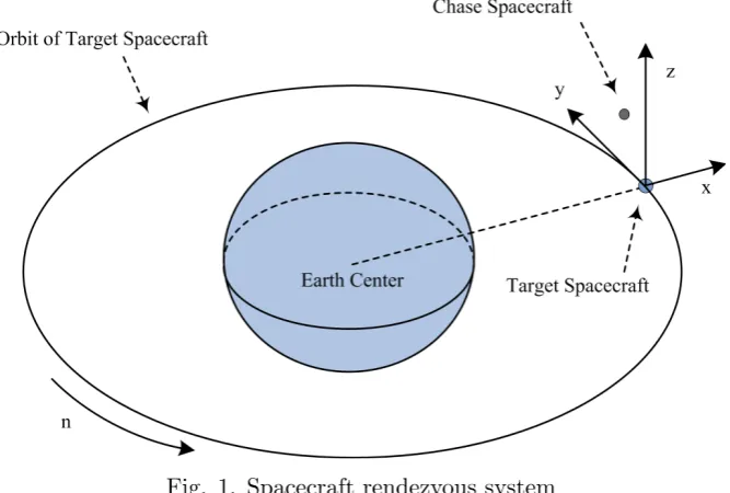
The spacecraft rendezvous system is illustrated in Fig. 1. We assume the two spacecraft (Target and Chaser) are adjacent, and the orbital coordinate frame in our study is a right-handed Cartesian coordinate, with origin attached to the target spacecraft center of mass, x-axis along the vector from earth center to the
target’s center of mass, y-axis along the target orbit circumference, and z-axis completing the right-handed frame.
Fig. 1. Spacecraft rendezvous system
The relative dynamic model can be described by C-W’s equations: 8
> < > :
•
x 2ny_ 3n2x= m1(Tx+!x);
•
y+ 2nx_ = m1(Ty+!y);
•
z+n2z= m1(Tz+!z);
(1)
wherex; y and z are the components of the relative position, n is the angle velocity of the target moving
around the earth,mis the mass of the chaser,Ti (i=x; y; z) is theithcomponent of the control input force acting on the relative motion dynamics, !i (i=x; y; z) is the ith component of the external disturbance.
disturbance vector!(t) = [!x; !y; !z]T;and output vectorf(t) = [x; y; z]T, we have (
_
q(t) =Aq(t) +Bu(t) +B!!(t);
f(t) =Cq(t); (2)
where A= 2 6 6 6 6 6 6 6 6 6 4
0 0 0 1 0 0
0 0 0 0 1 0
0 0 0 0 0 1
3n2 0 0 0 2n 0
0 0 0 2n 0 0
0 0 n2 0 0 0
3 7 7 7 7 7 7 7 7 7 5
; B=B!=
1 m 2 6 6 6 6 6 6 6 6 6 4
0 0 0
0 0 0 0 0 0 1 0 0
0 1 0 0 0 1
3 7 7 7 7 7 7 7 7 7 5
; C =
2 6 6 6 6 6 6 6 6 6 4
1 0 0
0 1 0 0 0 1 0 0 0
0 0 0 0 0 0
3 7 7 7 7 7 7 7 7 7 5 T :
The whole rendezvous process can be described by the transformation of state vector q(t) from nonzero initial stateq(0)to the terminal state q(tm) = 0;where tm is the rendezvous time.
In order to meet the requirements of actual conditions, the following important aspects should be taken into consideration simultaneously:
(1) Parameter uncertainty. Due to the detection errors or the complex force among the objects in
space, the angle velocity of target spacecraftncannot be determined online accurately. It can be generally characterized as
n=n0(1 + ); (3)
wheren0 is the theoretical angle velocity, and denotes the magnitude of uncertainty.
(2) Input constraint. In view of the limited power of actuator, the actual control input force should be
con…ned into a certain range, which means that
ku(t)k2 umax; (4)
whereumax denotes the maximum input force.
(3)Pole assignment. In order to obtain a desired dynamic performance of the closed-loop system, usually
the poles placement needs to be imposed. Here, we consider the disk regional poles constraint, and letf( ; r)
denote the disk region centered in with radius r in the complex plane ( ; r2Rand r >0). According to the parameter uncertainty, we have
_
where
~
A = A0+ A;
A0 =
2 6 6 6 6 6 6 6 6 6 4
0 0 0 1 0 0
0 0 0 0 1 0
0 0 0 0 0 1
3n2
0 0 0 0 2n0 0
0 0 0 2n0 0 0
0 0 n20 0 0 0
3 7 7 7 7 7 7 7 7 7 5 ; A = 2 6 6 6 6 6 6 6 6 6 4
0 0 0 0 0 0
0 0 0 0 0 0
0 0 0 0 0 0
3n20(2 + 2) 0 0 0 2 n0 0
0 0 0 2 n0 0 0
0 0 n2
0(2 + 2) 0 0 0
3 7 7 7 7 7 7 7 7 7 5 :
For the uncertain matrix Ain (5), we assume the norm-bounded condition
k Ak ; (6)
where is positive which can be determined by :
Now, we consider the following controller structure:
u(t) =Kq(t); (7)
whereK is a constant feedback control gain to be determined. Then, the resulting closed-loop system (5)
with (7) can be written as (
_
q(t) =Aq(t) +B!!(t);
f(t) =Cq(t); (8)
where A = ~A+BK. Our objective in this paper is to determine the controller gain K, such that the system in (8) is robustly stable and the performancekTf !k1 < is guaranteed subject to the parameter
uncertainties, external disturbance and input constraints, and the poles of the closed-loop system lie inside the disk regionf( ; r), wherekTf !k1denotes the closed-loop transfer function from!(t)tof(t), andf( ; r) denotes the disk region centered in with radius r in the complex plane. It can be brie‡y summarized as
the following minimization problem:
min s.t. 8 > < > :
the closed-loop system is stable and kTf !k1< ;
ku(t)k2 umax; OC;
where umax is a given constant, and OC represents other constraints, such as the poles constraint of the
closed-loop system.
Remark 1 In this paper, we only consider the state-feedback control problem, and it is assumed that the
real-time state signals can be transmitted accurately. It is worth mentioning that the output-feedback control problem is more important in real application, and the possible data missing phenomena should also be taken into consideration [31]. For spacecraft rendezvous, the output-feedback control problem with possible missing
Remark 2 It is known that the transient response of a linear system is related to the location of its poles.
By constraining the poles to lie in a prescribed region, speci…c bounds can be put on these quantities to ensure a satisfactory transient response. Till now, many di¤ erent kinds of poles regions have been studied, such as vertical strip, elliptical and hyperbolic regions. The circular region has been proved to be more e¤ ective in both
theory and practice, see, for instance [29], [30] and [32]. Readers are referred to [3] for more information about how to select the circular region.
3
Controller Design
In this section, we will investigate the multi-objective robustH1 state-feedback controller design problem. The design requirements mentioned above will be analyzed separately, and the obtained results will be utilized for the controller design. First, we recall the following results which will be used in our later
development, and their proofs and the applications can be found in [1], [2], [8], [9], [14], and [28].
Lemma 1 Let L,E andF are real matrices of appropriate dimensions withkFk 1:Then, for any scalar >0; we have
LF E+ETFTLT 1LLT + ETE:
Lemma 2 Let M andN be real matrices of appropriate dimensions, for any scalar " >0;
"
0 N MT
M NT 0
# "
"N NT 0 0 " 1M MT
#
:
Lemma 3 (Projection Lemma): Let ; and be given, there exists a matrix F satisfying
+ F T + FT T <0;
if and only if
? ?T <0; ? ?T <0:
In the multi-objective synthesis, in order to cast the controller design into a convex optimization problem,
we usually need to set a common Lyapunov matrix for di¤erent performance objectives. This method is simple, but is inevitably conservative due to the …xed positive symmetric matrix. In the following, we will
present a new approach which is potentially less conservative. Firstly, we will present three propositions, which convert the design requirements (H1performance, poles assignment and input constraints) into LMI conditions respectively.
Proposition 1 Consider the system in (8) and the state feedback control law in (7). The closed-loop system is stable and kTf !k1< if and only if there exist positive symmetric matrix P1, general matricesF andG
satisfying 2
6 6 6 6 4
ATG+GTA GTB! CT
F FT FTB
! 0
I 0
I
3 7 7 7 7 5
<0; (9)
where A= ~A+BK; =P1 GT +A
T
Proof. By de…ning = [G F], the inequality (9) can be written as
+ T + T T <0; (10)
where = 2 6 6 6 6 4
0 P1 0 CT
0 0 0
I 0 I 3 7 7 7 7 5; =
2 6 6 6 6 4 AT I B!T 0 3 7 7 7 7 5; =
2 6 6 6 6 4 I 0 0 I 0 0 0 0 3 7 7 7 7 5:
The orthogonal complements of and T are
?=
2 6 4
I AT 0 0
0 BT
! I 0
0 0 0 I
3 7
5; ?=
"
0 0 I 0
0 0 0 I
#
:
It is obvious that ? ?T <0:Then, by Lemma 3, it can be seen that (10) holds if and only if
? ?T =
2 6 4
ATP1+P1A P1B! CT
I 0
I
3 7
5<0: (11)
According to [3], the system in (8) is stable andkTz!k1< if and only if (11) holds, which, together with the equivalence between (9) and (11), completes the proof.
Proposition 2 Consider the closed-loop system in (8) and the state feedback control law in (7), assuming
that the initial stateq(0) is known, and given the positive symmetric matrixP1 introduced in Proposition 1.
Then, for allt 0; the input constraintku(t)k2 umax can be ensured if there exist general matrix V and
positive scalar satisfying
"
u2maxI K KT 1P1
#
0; (12)
"
I qT(0)V
VTq(0) VT +V P1
#
0: (13)
Proof. De…ne a Lyapunov functionU(q(t)) =qT(t)P1q(t), which satis…es
U(q(t)) ;
where is a given positive scalar. Denote the ellipsoid (P1; ) = q(t)jqT(t)P1q(t) . For ku(t)k2
umax, denote another ellipsoid (K) = q(t)j qT(t)KTKq(t) u2max . Thus, it can be seen that the input
constraints can be ensured by
(P1; ) (K): (14)
According to [4], we can see that (14) can be guaranteed if and only if
which can be readily obtained from (12) by Schur complement. At the same time, forP1 is introduced by
Proposition 1 which guaranteesU_(q(t))<0, then we haveq(t)TP1q(t)< q(0)TP1q(0) for t >0. Thus, the
conditionq(t)TP1q(t) can be ensured byq(0)TP1q(0) , which is equivalent to
"
I qT(0)
q(0) P1 1
#
0: (15)
Pre- and post-multiplying (15) bydiagfI; VTg and its transpose respectively, we obtain "
I qT(0)
q(0) VTP1 1V
#
0: (16)
For (P1 V)TP1 1(P1 V) 0, we have VTP1 1V VT +V P1: Then, it is obvious that (16) can
be ensured by (13). Thus, we can see that the conditions (12) and (13) can ensure (P1; ) (K) and q(t)TP
1q(t) , which renders the input constraints to be respected. The proof is completed.
Proposition 3 Consider the system in (8). All the poles of the closed-loop system lie inside the disk region
f( ; r) (centered in with radius r in the complex plane) if there exist positive symmetric matrix P2 and
general matrixH satisfying "
P2 HT H HT A I
r2P2
#
<0: (17)
Proof. For(P2 H)TP2 1(P2 H) 0;we have
HP2 1HT P2 HT H:
Then, it can be seen that if (17) holds, thenH is invertible and "
HTP2 1H HT A I
r2P2
#
<0: (18)
Pre- and post-multiplying (18) bydiagfP2H T; Ig and its transpose respectively, we obtain
"
P2 P2 A I
r2P2
#
<0: (19)
According to [3], the poles of the closed-loop system in (8) lie inside the disk region f( ; r) (centered in with radiusr in the complex plane) if and only if (19) holds, which can be ensured by (17). The proof is completed.
Propositions 1-3 formulate the conditions under which the closed-loop system meets the multi-objectives. Based on these propositions, the following theorem presents a controller design method via convex optimiza-tion.
Theorem 1 For the uncertain rendezvous system in (8) and a given scalar > 0, under the constraint
poles lie inside the disk regionf( ; r)(centered in with radiusrin the complex plane), if there exist scalars
i (i= 1;2;3); and >0; "j >0 (j= 1;2;3);and matrices S; L; P~k >0 (k= 1;2)satisfying
2 6 6 6 6 6 6 6 6 6 4
11 12 2B! STCT 1ST 2ST
22 1B! 0 0 0
I 0 0 0
I 0 0
"1I 0 "2I
3 7 7 7 7 7 7 7 7 7 5
<0; (20)
"
u2maxI L 1Pe
1
#
0; (21)
"
4qT(0)
4S+ 4ST Pe1
#
0; (22)
2 6 4
11 12 0
r2Pe2 ST "3I
3 7
5<0; (23)
where
11 = 2STAT0 + 2A0S+ 2BL+ 2LTBT +"2 2I;
12 = Pe1 2S+ 1STAT0 + 1LTBT;
22 = 1S 1ST +"1 2I;
11 = Pe2 3S 3ST +"3 23 2I;
12 = 3A0S+ 3BL 3 S:
Furthermore, the desired robust H1 state feedback control law is given by u(t) =LS 1q(t):
Proof. For the general matrices in Propositions 1–3, we select F , 1V; G , 2VT; H , 3V and S,V 1:Then, condition (9) in Proposition 1 can be rewritten as
2 6 6 6 6 4
2VTA+ 2ATV 2VTB! CT
1V 1VT 1VTB! 0
2I 0
I 3 7 7 7 7
5<0; (24)
where
=P1 2VT + 1A
T
V:
Pre- and post-multiplying (24) bydiag ST; ST; I; I and its transpose respectively, we obtain 2 6 6 6 6 4
2STA
T
+ 2AS 2B! STCT
1ST 1S 1B! 0
I 0 I 3 7 7 7 7
5<0; (25)
where
=STP1S 2S+ 1STA
T
Here, we de…nePe1,STP1S; L,KS;and then we have
2 6 6 6 6 4
11 12 2B! STCT
1ST 1S 1B! 0
I 0
I
3 7 7 7 7 5
<0; (26)
where
11 = 2A0S+ 2STAT0 + 2BL+ 2LTBT + 2 AS+ 2ST TA;
12 = Pe1 2S+ 1STA0T + 1ST TA+ 1LTBT:
By Lemma 2 and (6), for any scalar"1 >0;
"
# 1ST TA
&
# "
# +"11 21STS 0
& +"1 2I
#
; (27)
where # and & represent the original corresponding matrix elements in (26). And by Lemma 1 and (6), with scalar"2 >0;
2 AS+ 2ST TA "2 A TA+"21 2 2STS
"2 2I+"21 22STS: (28)
Thus, considering (26), (27) and (28), and by Schur complement, we can see that (24) can be ensured if (20)
holds, which means that the stability andH1performance can be guaranteed by (20).
Next, consider the conditions in Proposition 2. Pre- and post-multiplying (12) and (13) bydiag I; ST
and its transpose respectively, we can readily obtain the equivalent conditions (21) and (22), which can ensure the input constraints.
Finally, for H= 3V, (12) in Proposition 3 can be rewritten as
"
P2 3VT 3V 3VT A I
r2P2
#
<0: (29)
Pre- and post-multiplying (29) bydiag ST; ST and its transpose respectively, and by de…ningPe
2 =STP2S;
we obtain " e
P2 3S 3ST 3A0S+ 3 AS+ 3BL 3 S r2Pe2
#
<0: (30)
By Lemma 2 and (6), there exists scalar "3 >0 satisfying
"
# 3 AS
&
# "
# +"3 23 2I 0
& +"31STS
#
; (31)
where # and & represent the original corresponding matrix elements in (30). Thus, considering (30) and
(31), and by Schur complement, we can obtain (29) if (21) holds, which means that the poles constraint can be guaranteed by (23).
Thus, we can see that all the conditions listed in Proposition 1–3 can be ensured by (20)–(23), which
Remark 3 The scalar can be included as an optimization variable to obtain a reduction of the H1
disturbance attention level bound. Then, the minimumH1disturbance attention level bound in terms of the
feasibility of admissible controllers can be readily found by solving the following convex optimization problem:
Minimize subject to the LMIs in Theorem 1 (32)
4
Illustrative Example
In this section, we provide an example to illustrate the usefulness and advantage of the controller design
method proposed in the above sections. Here, we consider a pair of adjacent spacecraft, and make the following assumptions. The mass of the chaser is300kg; and the target is moving along a geosynchronous orbit of radiusr= 42241kmwith an orbital period of24hours. Thus, the angle velocityn0 = 7:2722 10 5
rads/s. Assume that the initial relative position (x0; y0; z0) = (800;600;500) at time t = 0: Furthermore,
for simplicity, we assume that the initial stateq(0) = [800;600;500;0;0;0];which means that the spacecraft
are relatively static before timet= 0. Assume that the maximum input control force is 3000N: Then, our purpose is to design a state feedback controller K in the form of u(t) = Kq(t); such that the closed-loop system satis…es
(1) stable and kTf !k1< ;
(2)ku(t)k2 3000;
(3) all the poles lie inside the disk regionf( 1;1)(centered in 1 with radius1 in the complex plane). First, we consider the situation without external perturbations (!(t) = 0) and assume = 0:01. By solving the convex optimization problem in (32), we obtain the associated matrices as follows (for brevity,
we only list the matrices necessary for the construction of the admissible controllers):
S=
2 6 6 6 6 6 6 6 6 6 4
0:5271 0:0310 0:0258 0:0308 0:0048 0:0041
0:0310 0:5448 0:0194 0:0049 0:0336 0:0030
0:0257 0:0194 0:5520 0:0040 0:0031 0:0347
0:0414 0:0032 0:0026 0:0074 0:0001 0:0001
0:0031 0:0432 0:0020 0:0001 0:0075 0:0001
0:0026 0:0020 0:0439 0:0001 0:0001 0:0075
3 7 7 7 7 7 7 7 7 7 5
;
L=
2 6 4
0:2482 0:1024 0:0853 0:0972 0:0094 0:0078
0:1028 0:1891 0:0643 0:0094 0:1025 0:0059
0:0854 0:0641 0:1653 0:0078 0:0059 0:1047
3 7 5:
Therefore, the gain matrix for the feedback controller is given by
K =L S 1 =
2 6 4
2:2541 0:0071 0:0072 22:3975 2:3256 1:9369
0:0104 2:2493 0:0055 2:3259 23:7456 1:4544
0:0072 0:0055 2:2471 1:9357 1:4552 24:2818
3 7 5:
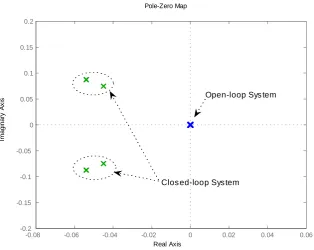
With the controller K, we consider the poles assignment of the closed-loop system. Fig. 2 illustrates the
-0.08 -0.06 -0.04 -0.02 0 0.02 0.04 0.06 -0.2
-0.15 -0.1 -0.05 0 0.05 0.1 0.15 0.2
Pole-Zero Map
Real Axis
Im
ag
ina
ry
A
x
is Open-loop Sys tem
Clos ed-loop Sys tem
Fig. 2. Poles of open- and closed-loop systems.
We can see that all the poles of open-loop system are near by the origin, which means the weak stability of
the system. And we can see that all the poles of the closed-loop system have been aparted from the imagine axis, and have been placed into the expected regionf( 1;1). So the requirement of poles assignment can be satis…ed by the designed controller.
Next, we assume = 0:002and the following external disturbance signal:
!(t) =
(
10 sin 0:2t; 0< t <60s,
0; otherwise.
By solving the convex optimization problem in (32), the gain matrix for the feedback controller is given by
K=
2 6 4
1:9770 0:0300 0:0237 23:4372 0:7655 0:6378
0:0270 1:9939 0:0177 0:7695 23:8812 0:4796
0:0237 0:0177 2:0004 0:6392 0:4804 24:0589
3 7 5;
and min = 4:9678. The output of the closed-loop system (which means the relative position of the two
0 20 40 60 80 100 120 140 160 -200
-100 0 100 200 300 400 500 600 700 800
tim e / s
ou
tp
ut
/ m
Zx
Zy Zz
Fig. 3. The output of system (which also means the relative position of the two satellites)
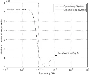
Generally, the expected attitude and orbit of spacecraft are always heavily a¤ected by low frequency
distur-bance force. Thus, it is necessary to investigate the frequency response of the system during the controller design. Fig. 4 shows the open- and closed-loop frequency responses from the disturbance!(t) to the out-put z(t): The zoomed area is depicted clearly in Fig. 5. It can be seen that the response of very low
frequency disturbance is huge in open-loop system, which is unacceptable in practice. And we can see that the closed-loop system has signi…cant reduction in amplitude compared with the open-loop system.
10-10 10-8 10-6 10-4 10-2 100 0
1 2 3 4 5 6 7x 10
5
Frequency / Hz
M
ax
im
um
pos
it
ional
res
pons
e
/
m
Open-loop Sys tem Clos ed-loop Sys tem
be s hown in Fig. 5
Fig. 4. Overview of the frequency responses of open- and closed-loop system from disturbance to the
10-4 10-3 10-2 0.2
0.4 0.6 0.8 1 1.2 1.4 1.6 1.8
Frequency / Hz
Max
imum pos
iti
onal
r
es
po
ns
e
/
m
Open-loop System Closed-loop System
Fig. 5. Zoomed area of frequency responses of open- and closed-loop system from disturbance to the positional output
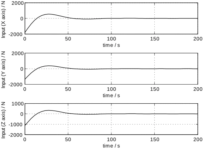
Furthermore, the maximal control input force must be investigated due to its constraint. The variations of control input force in three axes are depicted in Fig. 6. From the …gure, we can see that the input force
component in x-axis is the largest, which is obvious due to the initial state (the position component in x-axis is the largest when t = 0). And we can see that even the largest input force of three axes is bellow the maximum allowed force3000N;which means that the input constraints can be guaranteed by the designed
controller.
0 50 100 150 200
-2000 0 2000
tim e / s
In
pu
t
(X
a
x
is
) /
N
0 50 100 150 200
-2000 0 2000
tim e / s
In
pu
t
(Y
a
x
is
) /
N
0 50 100 150 200
-2000 -1000 0 1000
tim e / s
In
pu
t
(Z axi
s
) / N
Fig. 6. Control input force in three axises
rendezvous process. It can be shown that the two spacecraft will eventually asymptotically rendezvous.
-50 -40 -30 -20 -10 0 10 20 30 -50
0 50 -25 -20 -15 -10 -5 0 5 10 15 20
← Target
x / m rendezvous orbit→
y / m
z
/ m
Fig. 7. Approximate rendevzous orbit in the …nal peroid
5
Conclusions
This paper has presented a new robustH1state-feedback controller design method for spacecraft rendezvous subject to parameter uncertainty, external perturbation, input constraints and poles assignment. By using
Lyapunov method and linear matrix inequality techniques, the multi-objective design problem has been transformed into a convex optimization problem with linear matrix inequality constraints. An illustrative example has shown the e¤ectiveness of the proposed controller design methods.
References
[1] M. V. Basin and A. E. Rodkina. On delay-dependent stability for a class of nonlinear stochastic delay-di¤erence equations. Dynamics of Continuous, Discrete and Impulsive Systems, 12(5):663–675,
2005.
[2] M. V. Basin and A. E. Rodkina. On delay-dependent stability for a class of nonlinear stochastic systems
with multiple state delays. Nonlinear Analysis: Theory, Methods and Applications, 68(8):2147–2157, 2007.
[3] S. Boyd, L. El Ghaoui, E. Feron, and V. Balakrishnan. Linear Matrix Inequalities in Systems and
Control Theory. SIAM, Philadelphia, PA, 1994.
[4] Y. Y. Cao and Z. Lin. Robust stability analysis and fuzzy-scheduling control for nonlinear systems
[5] W. H. Clohessy and R. S. Wiltshire. Terminal guidance system for satellite rendezvous. Journal of
Aerospace Science, 27(9):653–658, 1960.
[6] V. Coverstone-Carroll, J. W. Hartmann, and W. J. Mason. Optimal multi-objective low-thrust
space-craft trajectories. Computer Methods in Applied Mechanics and Engineering, 186:387–402, 2000.
[7] B. Ebrahimi, M. Bahrami, and J. Roshanian. Optimal sliding-mode guidance with terminal velocity constraint for …xed-interval propulsive maneuvers. Acta Astronautica, 60(10):556–562, 2008.
[8] H. Gao and T. Chen.H1estimation for uncertain systems with limited communication capacity.IEEE
Transactions on Automatic Control, 52(11):2070–2084, 2007.
[9] H. Gao, J. Lam, C. Wang, and Y. Wang. Delay-dependent output-feedback stabilisation of discrete-time systems with time-varying state delay. IEE Proceedings Control Theory & Application, 151(6):691–670,
2004.
[10] H. Gao, P. Shi, and J. Wang. Parameter-dependent robust stability of uncertain time-delay systems.
Journal of Computational and Applied Mathematics, 206(1):366–373, 2007.
[11] H. Gao and C. Wang. A delay-dependent approach to robust H1 …ltering for uncertain discrete-time state-delayed systems. IEEE Transactions on Signal Processing, 52(6):1631–1640, 2004.
[12] G. W. Hughes and C. R. McInnes. Solar sail hybrid trajectory optimization for non-keplerian orbit
transfers. Journal of Guidance Control and Dynamics, 25(3):602–604, 2002.
[13] D. J. Jezewski and J. D. Donaldson. An analytical approach to optimal rendezvous using
clohessy-wiltshire equations. Journal of Astronautical Sciences, 27(3):293–310, 1979.
[14] P. P. Khargonekar, I. R. Petersen, and K. Zhou. Robust stabilization of uncertain linear systems: quadratic stabilizability and H1 control theory. IEEE Transactions on Automatic Control, 35:356– 361, 1990.
[15] C. A. Kluever. Optimal low-thrust interplanetary trajectories by direct method techniques. Journal of
Astronautical Sciences, 45(3):247–262, 1997.
[16] C. A. Kluever. Comet rendezvous mission design using solar electric propulsion spacecraft. Journal of
Spacecraft and Rockets, 37(1):698–700, 2000.
[17] Y. Z. Luo and G. J. Tang. Spacecraft optimal rendezvous controller design using simulated annealing.
Aerospace Science and Technology, 9:732–737, 2005.
[18] Y. Z. Luo, G. J. Tang, and Y. J. Lei. Optimal multi-objective linearized impulsive rendezvous. Journal
of Guidance Control and Dynamics, 30(2):383–389, 2007.
[19] G. Mengali and A. A. Quarta. Fuel-optimal, power-limited rendezvous with variable thruster e¢ ciency.
Journal of Guaidance Control and Dynamics, 28(6):1194–1199, 2005.
[20] D. S. Naidu. Fuel-optimal trajectories of aeroassisted orbital transfer with plane change. IEEE
[21] W. Scheel and B. A. Conway. Optimization of very-low-thrust, many-revolution spacecraft trajectories.
Journal of Guaidance Control and Dynamics, 17(6):1185–1192, 1994.
[22] P. Shi and K. Boukas. OnH1control design for singular continuous-time delay systems with parametric
uncertainties. Journal of Nonlinear Dynamics and Systems Theory, 4(1):59–71, 2004.
[23] P. Shi, K. Boukas, and R. Agarwal. Control of markovian jump discrete-time systems with norm bounded uncertainty and unknown delay. IEEE Transactions on Automatic Control, 44(11):2139–2144, 1999.
[24] P. Singla, K. Subbarao, and J. L. Junkins. Adaptive output feedback control for spacecraft rendezvous
and docking under measurement uncertainty. Journal of Guaidance Control and Dynamics, 29(4):892– 902, 2006.
[25] G. L. Tang, Y. Z. Luo, and H. Y. Li. Optimal robust linearized impulsive rendezvous.Aerospace Science
and Technology, 11:563–569, 2007.
[26] A. Tiwari, J. Fung, J. M. Carson, R. Bhattacharya, and R. M. Murray. A framework of lyapunov certi…cates for multi-vehicle rendezvous problems.Proceeding of the 2004 American Control Conference,
Boston, Massachusetts, pages 5582–5587.
[27] J. Wang, P. Shi, and H. Gao. Gain-scheduled stabilization of linear parameter-varying systems with time-varying input delay. IET Control Theory & Applications, 1(5):1276–1285, 2007.
[28] Y. Wang, L. Xie, and C. E. de Souza. Robust control of a class of uncertain nonlinear systems.Systems and Control Letters, 19:139–149, 1992.
[29] Z. Wang. Robust H1 state feedback control with regional pole constraints: An algebraic riccati
equation approach. Journal of Dynamic Systems Measurement and Control-Transactions of the ASME, 120(2):289–292, 1998.
[30] Z. Wang, G. Tang, and X. Chen. Robust controller design for uncertain linear systems with circular pole constraints. International Journal of Control, 65(6):1045–1054, 1996.
[31] Z. Wang, F. Yang, D. W. C. Ho, and X. Liu. RobustH1 control for networked systems with random packet losses. IEEE Transactions on System, Man and Cybernetics-Part B: Cybernetics, 37(4):916–924,
2007.