The effect of school quality on educational attainment and wages

(1)

The Review of Economics and Statistics

V

OL

. LXXXIV

F

EBRUARY

2002

N

UMBER

1 THE EFFECT OF SCHOOL QUALITY ON EDUCATIONAL

ATTAINMENT AND WAGES

Lorraine Dearden, Javier Ferri, and Costas Meghir

Abstract—The paper examines the effects of pupil-teacher ratios and type of school on educational attainment and wages using the British National Child Development Survey (NCDS). The NCDS is a panel survey that follows a cohort of individuals born in March 1958 and has a rich set of background variables recorded throughout the individuals’ lives. The results suggest that, once we control for ability and family background, the pupil-teacher ratio has no impact on educational qualifications or on men’s wages. It has an impact on women’s wages at the age of 33, particularly those of low ability. We also find evidence that those who attend selective schools have better educational outcomes and, in the case of men, higher wages at the age of 33. The impact is greater for the type of individuals who are less likely to attend selective schools but for whom a comparison group does exist among those attending.

I. Introduction

T

HIS paper examines the impact of measures of inputs

into schooling (often referred to as “school quality”) on educational attainment, hourly wage rates at 23 and 33 years of age, and employment. We use a unique data set for this purpose that, due to its rich array of characteristics, allows us to address many of the concerns raised in the school quality literature. This data set follows a cohort of individ-uals born in a week of 1958.

There is much controversy over whether particular as-pects of school quality that are directly affected by govern-ment policy have significant effects on an individual’s future educational achievement and earnings. The measures of school quality or school inputs that are typically central to this debate include pupil-teacher ratios, expenditure per pupil, and measures of teacher quality, such as average teacher salaries. Most of the literature looking at school quality stems from the United States, and it began with the publication of the Coleman Report in 1966 (Coleman et al., 1966). The controversial finding of this report was that

measured school quality had very little effect on pupil achievement once family background and school composi-tion effects had been taken into account. The subsequent U.S. literature looking at this issue has, on the whole, tended to confirm this somewhat surprising finding, or at best found only weak effects of school quality on pupil achievement. (See, for example, Hanushek (1986) and Hanushek, Rivkin, and Taylor (1996).)

As Moffitt (1996) points out, a separate strand of the school quality literature has instead focused on the impact of school quality on later earnings. The findings from this strand of the school quality debate have, on the whole, found significant impacts of school quality on later earnings in distinct contrast to the pupil achievement literature. (See, for example, the papers by Johnson and Stafford (1973) and Card and Krueger (1992).) Some quite recent contributions to this literature have, however, found no significant effects (for example, Betts (1995) and Heckman, Layne-Farrar, and Todd (1996)). There are a number of differences between the various studies in type of data and in the way they are used that could be at the root of the differences.

A possible explanation for the different findings is that the effect of school quality has been declining over time and/or is less important for younger workers than it is for older workers. Most of the analyses looking at pupil achievement have focused on relatively young cohorts of individuals, born in the 1950s or later, while they are early in their careers, whereas the studies focusing on earnings have tended to concentrate on older cohorts of individuals who are later in their working life (aged 30 or above). Card and Krueger (1992), for example, focus on a cohort of individuals born in the 1920s, 1930s, and 1940s and aged between 30 and 60 in 1980, whereas the study by Betts (1995) focuses on men aged 32 or younger. Loeb and Bound (1996) look at the issue of whether school quality effects on achievement have been declining over time by examining a cohort of men born in the United States in the 1920s, 1930s, and 1940s. They find that state-level measures of school quality have a significant effect on pupil achievement for this group of individuals. They argue that this finding may, in part, reflect differences across cohorts but that it also may reflect the extent of aggregation involved in measuring school inputs in their study. Betts (1996) looks at the issue

Received for publication January 27, 1998. Revision accepted for publication February 13, 2001.

Institute for Fiscal Studies, Universitat de Vale`ncia, and University College London and Institute for Fiscal Studies, respectively.

We thank two anonymous referees, Christian Dustmann, James Heck-man, Paul Johnson, the editor Robert Moffitt, Steve Pischke, Chris Pissarides, and Petra Todd for useful comments and stimulating discus-sions. Participants in seminars at CREST-INSEE and CEP-LSE provided useful comments. Costas Meghir’s work on this paper was largely under-taken while he was visiting CREST-INSEE in Paris. Lorraine Dearden’s work on this paper was funded under Leverhulme Trust Research Grant F/386/G. We thank CREST, the ESRC Centre for the Microeconomic Analysis of Fiscal Policy at the Institute for Fiscal Studies, and the Leverhulme Trust for financial support.

The Review of Economics and Statistics, February 2002, 84(1): 1–20

(2)

of whether school quality effects increase with age and labor market experience. He uses both individual-level and state-level census data and finds that there is no evidence of age dependence.

Another explanation relates to the importance of factors such as family background and ability in determining choice of school, as well as pupil achievement and earnings. If this is not taken into account, the estimated relationship between school quality and earnings and/or achievement may be spurious. Very few studies in the school quality literature have directly addressed this problem because of a lack of suitable data. The original Coleman Report explicitly con-trolled for individuals’ socioeconomic characteristics as well as school composition and found that these factors were much more important determinants of pupil achieve-ment than were quality measures. Two recent studies have used sibling (Altonji & Dunn, 1996) and twin (Behrman, Rosenzweig, & Taubman, 1996) data to look at this issue. If some siblings or twins attend different schools, the data can be used to look at the impact of differences in school quality on differences in earnings. In these models, unobserved family effects with the same impact on all siblings will be differenced out. Altonji and Dunn (1996) find that school quality effects on earnings increase when such family-fixed effects are controlled for, whereas Behrman et al. (1996) find that college quality effects on earnings are decreased.

In this paper, we use data from England and Wales1 _to

examine the impact of the pupil-teacher ratio and type of school on educational achievement, employment, and hourly wages at two different ages (23 and 33). We use a unique data set, the National Child Development Survey (NCDS), which is a continuing longitudinal study of all subjects living in Great Britain who were born in the week of March 3–9, 1958. There have been five follow-up sur-veys for this cohort, the latest in 1991 when the individuals were aged 33. The surveys have detailed information on the individuals’ educational achievements (both school and post-school), family backgrounds, and labor market histo-ries. Importantly for the purpose of this paper, the data set also has information obtained from the individuals’ schools at the ages of 7, 11, and 16 on measures such as the pupil-teacher ratios and class sizes, type of school (such as state selective, state nonselective, or private, and single-sex or coeducational) and results of numerous ability tests undertaken by the individuals at the time of each of the follow-up surveys, as well as the families’ financial circum-stances and compositions.

The paper looks at the effect of the pupil-teacher ratio and school type on educational achievement and earnings at two points in the life cycle: ages 23 and 33. The importance of controlling for ability and family background, which are

often unobserved, can therefore be assessed directly. The age dependence of the effect of the pupil-teacher ratio can

also be explicitly examined.2

Other studies that consider the effects of school quality on outcomes are Dustmann, Rajah, and Van Soest (1997), who focus on the effects of school quality on continuation of education beyond sixteen, Robertson and Symons (1996), who attempt to measure the effects of peer groups on school performance, and Feinstein and Symons (1999), who study attainment in secondary schools. Our focus is on outcomes later on, that is, on the ultimate educational attainment and on labor market performance.

In section II of the paper, we outline our methodological approach. Section III takes a closer look at the NCDS data used in the paper. We discuss our empirical results in section IV. Section V concludes and considers the important policy implications of our analysis.

II. Methodological Approach

Our methodology involves a sequential approach. We begin by examining the effect of school quality measures and other factors on educational attainment. We then exam-ine the effects of our school quality measures on wages at two points in the life cycle ten years apart, conditional on the highest qualification obtained up to that point. Finally, we look at the effect of school quality on the probability of being employed. By taking this sequential approach, we can assess the effects of school quality on outcomes through three main channels: educational attainment, the level of wages, and the returns to potential experience. We also consider the effect of school inputs on wages without conditioning on qualifications. This allows us to measure the total impact, comprising the direct effect and the effect that works through educational qualifications. We also ex-amine the effect of the pupil-teacher ratios in primary and in secondary school as well as the type of school, such as single-sex schools, private schools, and different types of state schools (selective and nonselective).

A number of important endogeneity issues need to be addressed in looking at the effect of school quality on both educational attainment and earnings. First, parents with a greater interest in their child’s education may locate close to schools that they consider to be better. They may use the pupil-teacher ratio as a factor. They may also choose single-sex schools for girls and mixed schools for boys simply because this is thought to be “best.” Because an active interest in the child’s education may lead to better educa-tional attainment and higher earnings, such self-selection

1_{We exclude individuals from Scotland because we use local education}

authority data in the paper, and these are only available on a consistent basis for England and Wales. Also, the Scottish schooling system differs from that of England and Wales.

2_{In an earlier version of the paper, we also considered the impact of the}

(3)

may generate an upward bias on school quality measures. If this is the case, our estimate of the pupil-teacher ratio effect may be too large due to nonrandom assignment to schools. Alternatively, a downward bias may be generated if parents whose children attend the better schools invest less of their time in their children’s education. Second, some types of schools select pupils by ability, which in itself is likely to imply that pupils from such schools will perform better and obtain higher qualifications. This is certainly the case for most private schools and for the state grammar schools. In the two examples just given, the bias is generated by the active choices of parents and schools.

Another source of bias may originate in the way that education is financed in the United Kingdom. In England and Wales, the responsibility for schooling is shared be-tween central government and local education authorities (LEAs). In 1974, there were 117 LEAs in England and Wales. Central government provides LEAs with resources to fund education (and other local services), and LEAs with an economically disadvantaged population receive higher

government grants.3 _{It is up to the LEA to determine how}

much of this money they allocate to schools. Private schools do not receive government money and are funded by en-dowments and fee-paying pupils. Some of the extra educa-tion money given to LEAs with a more disadvantaged population is spent on providing things such as free school meals to disadvantaged pupils, and this forms part of the education budget. It may also be spent on reducing the pupil-teacher ratio. But children from deprived neighbor-hoods may perform worse, thus generating a downward bias on the effect of the pupil-teacher ratio on educational attainment. Finally, the local socioeconomic environment that the child lives in may affect educational attainment and/or future earnings (such as through role model or peer effects). If such characteristics are also correlated with measures of school quality, omitting them may generate a further source of bias.

In the absence of some obvious experimental framework (as in Krueger (1999)) allocating pupils randomly to differ-ent types of school, one way of solving such endogeneity problems would be to use some instrumental variables procedure. This requires exclusion restrictions. However, in this context, it is very hard to argue that any of the available background, family, or local variables determine school allocation but not educational attainment and wages. All such variables are potential inputs in the production of human capital.

In our view, the best way to deal with the endogeneity issues with data such as ours is to control for the variables that are likely to be driving school selection before the

relevant treatment occurs. Hence, on the basis of the previ-ous discussion, we need

● family background variables to control for differences

in parental circumstances and tastes for education (X1),

● individual characteristics and test scores to control for

differences in ability (X2),

● characteristics of the local authority to control for

variation in education expenditures related to the

amount of deprivation in the area (X3), and

● neighborhood characteristics (X4).

The NCDS data used in this study explicitly allow us to control for all of these effects, which makes the matching approach we use here credible. Such rich data have not been previously used in the school quality literature.

Formally, we wish to estimate the effect of school input

variables (Qi) on schooling or education (si) and (log)

wages (wi). We assume that any selection takes place on the

basis of observable variables Zi⫽ [X1i, X2i, X3i, X4i]. We

assume that conditioning on the observables (Zi) is

suffi-cient to control for the endogenous choice of school quality

(Qi). More formally, we have the following simple

sequen-tial model for two time periods ( j ⫽ 1, 2):

sji⫽␦j0⫹␦⬘j1Qi⫹␦⬘j2Zi⫹uji j⫽1, 2 (2.1)

wji⫽␤j0⫹␤⬘j1Qi⫹␤⬘j2Zi⫹␳⬘sji⫹vji, j⫽1, 2 (2.2)

where the␦j1and␤j1measure the effect of school quality on

our outcome variables sji and wji in 1981 ( j ⫽ 1) and in

1991 ( j ⫽ 2), respectively. In this model, we assume that

individuals who are the same in the observable dimension Zi

but who attended schools characterized by different values

of Qido not differ, on average, in the unobserved dimension

uji and vji. Formally, this means that E(uji兩Qi, Zi) ⫽

E(uji兩Zi), and E(vji兩Qi, Zi, sji) ⫽ E(vji兩Zi).

We can extend this simple model to allow the effects of school quality to be heterogeneous in the population (that is,

␦j1i⫽ ␦j1⫹ vji where Var (vji) ⬎0, and␤j1i⫽ ␤j1 ⫹ ⑀ji

where Var (⑀ji) ⬎ 0). We assume that, although the effects

of Qimay be heterogeneous in the population (that is, Var

(vji) ⬎ 0 and Var (⑀ji) ⬎ 0), only the average population

values of␦j1i and␤j1i, conditional on the observables, are

known by the person undertaking the choice of Qi for the

child. In other words, we assume that the parent does not

know the precise return of Qi to his or her own child.

Formally, we assume that E(vji兩Qi, Zi)Qi⫽E(vji兩Zi)Qiand

E(⑀ji兩Qi, Zi, sji)Qi ⫽ E(⑀ji兩Zi)Qi. Hence, the average

school quality effects,␦j1and␤j1, can be identified from the

following sequential regression models:

sji⫽␦j0⫹␦⬘j1Qi⫹␦⬘j2Zi⫹␦⬘j3共Zi 䊟 Qi兲⫹uji

j⫽1,2 (2.3)

3_{The Education Reform Act of 1988 allowed schools to opt out of LEA}

(4)

wji⫽␤j0⫹␤⬘j1Qi⫹␤⬘j2Zi⫹␤⬘j3共Zi 䊟 Qi兲

⫹␳⬘sji⫹vji j⫽1, 2

(2.4)

where E(uji兩Qi, Zi) ⫽ 0 and E(vji兩Qi, Zi, sji) ⫽ 0. In

equations (2.3) and (2.4), the coefficients␦j3and␤j3capture

the heterogeneity in the effects of Qi. The arguments used

here are similar to the arguments made for matching esti-mators (see Heckman, Ichimura, and Todd (1997)), al-though our approach is more restrictive in the sense that we use linear matching.

As pointed out in the previous model, we present results for wages with education achieved up to that point as a control variable. This is done to isolate the effect of the pupil-teacher ratio and type of school over and above their effect on the qualification obtained. However, we also present results for wages without the educational qualifica-tions included.

When using matching estimators, one should control for variables in the information set of agents making the deci-sion that will affect treatment (here, the pupil-teacher ratio and type of school). When we consider the primary school pupil-teacher ratio, we condition on family background and local characteristics describing the broader area and the local neighborhood. Test scores at age seven are obtained at the early stages of primary school, and they may already contain the effect of the primary pupil-teacher ratio. Thus, we report results with test scores at seven included and not included.

In the next part of the empirical results, we focus our attention on the effect of the secondary school pupil-teacher ratio and type of secondary school. When we do this, we control for test scores at seven and eleven years of age, as well as the other background variables. Of course, the test scores are themselves probably endogenous and a function of family background and earlier school inputs. Neverthe-less, when the secondary schooling decision is made, the test scores at seven and eleven are known by the decision-makers (parents and schools) and consequently the selection takes place possibly using these variables. Omitting them may confound the effect of the subsequent school inputs with the selection on these ability scores. In fact, our assumption that all selection is on observables (the match-ing assumptions) relies on includmatch-ing all those observables that are likely to affect the treatment decision. The fact that our data allow us to do this is the strength of our approach. However, we also report results that do not include some or all of the test scores.

Given these matching assumptions, the wage equation can be estimated by ordinary least squares (OLS). The standard errors must be estimated using White’s (1980) adjustment for heteroskedasticity, if only because the

heter-ogeneous returns imply that the variance of uji andvji will

depend on Qi.

For educational qualifications, we use an ordered probit. The basic assumption is that we can explain all education

choices using a single index given by the right-hand side of the regression in equation (2.1). Heckman and Cameron (1998) provide conditions under which this is a valid ap-proach. We also need to assume that our errors are ho-moskedastic. This assumption does not sit comfortably with the possibility of heterogeneous responses that depend on unobservables. A multinomial choice model incorporating seven education levels is, however, computationally com-plex. Instead, we assess the validity of the ordered probit assumption by comparing the results we get with those obtained by a simple probit model where the dependent variable is “obtain some qualifications” versus none. We also look at the top of the educational distribution by estimating another probit model for obtaining a degree versus no degree. Under the null hypothesis, the results of the two approaches should be similar. Under the alternative, they would differ because the probit does not impose the single index assumption across all education choices.

An important issue, particularly when we consider the

causal impact of school type,4_{is whether the composition of}

the population going to different types of schools is such that we can actually form comparison groups. We examine this issue in a separate section, and we also construct a nonparametric matching estimator for the effect of school type, taking particular care to impose common support when we compare children in selective and nonselective schools. We do this because we feel that school type may reflect important inputs in education.

III. The Data

For this study, we use the National Child Development Survey (NCDS), which charts the development of all chil-dren born in a week of March 1958. The data set contains information on the parents and a wealth of information on the subjects at six points in the life cycle: birth, 7, 11, 16, 23, and 33. The data contain information on family background, on ability test scores, on the characteristics and types of school attended at each interview date, on educational qualifications and training, on the area of residence at each survey date, on wages and hours worked (at ages 23 and 33), and on occupation. The initial sample covered 17,414 individuals, but there has been quite a lot of attrition since. In the subsequent waves, the sample sizes were 15,468, 15,503, 14,761, 12,537, and 11,409, respectively. In 1978, exam results were obtained for 14,370 subjects directly

4_{The three types of state secondary schools are comprehensive schools,}

(5)

from their schools. Dearden, Machin, and Reed (1997) show that attrition has tended to take place among individuals

with lower ability and lower educational qualifications.5_The

sample used in this paper under-represents individuals in the

bottom of the ability distribution.6 _{Attrition need not bias}

our results, however, to the extent that it depends on observables only. Given the large array of characteristics relating to ability and background, we have reasonable grounds to believe that, in our analysis, attrition is exoge-nous, given the observables.

A. Variables Used in the Analysis

School Quality Variables: From the NCDS, we observe the pupil-teacher ratio in the child’s school at age eleven (end of primary school) and sixteen (end of compulsory schooling), both collected directly from the school. Class size often reflects the needs of the particular class because schools use streaming by ability and tend to place children with greater learning difficulties in smaller classes. Because we cannot directly control for this with the NCDS data, we decided to use the overall pupil-teacher ratio in the school, which does not suffer from this endogeneity problem. Al-though it is still true that schools in more deprived areas will tend to have lower pupil-teacher ratios because of the extra funding they receive from central government, the data allow us to control directly for the level of deprivation in the child’s immediate neighborhood.

Rather than excluding pupils who went to private schools, as is often done in school quality studies (such as Card and Krueger (1992)), we keep them in the sample and include controls for the type of school in some of the regressions. With our large array of information on test scores and family background, we can control for the main relevant factors that govern selection into schools. We also control for whether the secondary school is single-sex or not. This dimension of schooling is an important issue in the United Kingdom.

Family Background Variables: We use data from the second and third waves of the survey to construct variables identifying

● the father’s occupation in 1974,

● the years of full-time education undertaken by the

child’s mother and father,

● a variable identifying individuals who had no father

figure in 1974,

● whether the child was receiving free school meals in

1969 and/or 1974,

● whether the family was experiencing serious financial

difficulties in 1969 and/or 1974, and

● the number of siblings and older siblings the individual

had in 1974.

We also include indicators of the parents’ interest in the child’s education as assessed by the primary-school teacher.

Ability Variables: We utilize the results from reading and mathematical ability tests undertaken when the person was aged seven and eleven. From these reading and math-ematical ability tests, we construct dummy variables

rank-ing the individual’s results in each of the tests by quintiles.7

Local Authority and Neighborhood Characteristics: All regressions presented include indicators for the ten broad administrative regions as well as a dummy for the inner London and outer London regions. We also include a set of variables that describe the immediate social environment in the child’s neighborhood, as well as the overall deprivation level of the local authority (municipality). These variables are taken from the 1971 census and relate to the enumera-tion district and to the local authority where the child lived in 1974. The enumeration district is small enough to pick up the characteristics of the child’s immediate neighborhood. The local authority variables cover a much larger area and are included to control for the fact that central government grants to local authorities (including education grants) relate to the level of LEA deprivation. Finally, we include a set of variables describing the size of the local authority and its

“needs.”8

Wage and Education Data: We use data from the fourth and fifth waves of the survey to construct real hourly gross wage data measured in 1995 prices. We limit our sample to individuals who are employees at the time of the 1981 and/or 1991 survey. Because all individuals in the sample were born in the same week of March 1958, age (or potential labor market experience) is controlled for in all of our models. Our other outcome variable is highest educa-tional qualification (based on both school and post-school qualifications) at the ages of 23 in 1981 and 33 in 1991. A

5_{See Dearden et al. (1997), tables 2a and 2b, pp. 53–54. The nature of}

attrition in the NCDS sample is discussed in detail in the documentation accompanying the various surveys.

6_{For example, only 16.5% of individuals (15.9% of men and 17.0% of}

women) in the sample used in this paper were in the bottom quintile of the math ability test undertaken at the age of seven, whereas 22.41% of individuals (24.6% of men and 20.4% of women) were in the top quintile of this math ability test. (See table A1 in the appendix.)

7_{We choose quintiles because 20% of individuals in 1965 when the tests}

were undertaken obtained maximum marks in the reading ability test. The quintiles refer to quintiles at the time the test was taken and not in our final sample. (See table A2 in the appendix.)

8_{The enumeration district variables we include are the proportions of}

(6)

full description of how this is constructed is given in table A1 in the appendix.

Individuals often work in different areas from the one in which they attended school. When estimating the wage equations, we include nine dummies for region of schooling at age 16. In the paper, we estimate two sets of wage equations, one at the age of 23 and one at the age of 33. In each case, we also include dummies for the region of residence at that age to control for the effects of the local labor market. We also include the highest qualification obtained by that age.

B. Descriptive Information from the Final Sample

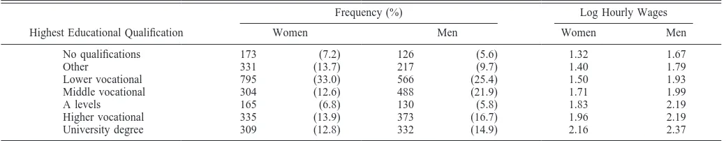
Table 1 shows the educational achievement of men and women by the age of 33. In the last two columns, we show the real log hourly wage in 1991 (in January 1995 prices) for each of the educational categories for the subsample of individuals for whom we have valid wages data.

A significant number of individuals in this cohort have ended up with only a low-level qualification, that is, more than 40% of men and more than 50% of women if we take the first three categories. Nevertheless, the rest have a higher qualification, which, as we see from log wages, is associated with large pay advantages. As an interesting aside, note that, in the raw data, there are very large male/female wage differentials at all educational levels, although these are likely to be explained in part by the differing levels of labor market experience at the age of 33. From table A2 in the appendix, we see that the pupil-teacher ratio is much more dispersed for primary schools than it is for secondary schools. For the largest sample, the average primary pupil-teacher ratio is 23.8 with a standard deviation of 9.5, compared with an average of 17.1 and a standard deviation of 2.0 for secondary schools. In table 2, we break down the pupil-teacher ratio in secondary schools

by school type and sex. There are four types of school. The 1968 Education Act allowed LEAs to establish nonselective state schools called “comprehensives.” Prior to this act, pupils had to take an exam at age eleven. The successful pupils (those in the top 10%–20%) went on to a grammar school, whereas the rest attended a secondary modern

school.9 _{Our cohort went through the education system as}

this reform was being implemented. In fact, grammar schools still survive in some areas today, and their revival is at the center of the education policy debate. The final category of schools are the private or independent schools, which are known in England and Wales as “public” schools. From table 2, it seems that private schools have the lowest pupil-teacher ratio, although the degree of dispersion is relatively large compared with the state sector. Secondary modern schools have the highest average pupil-teacher ratio. Women went through schools with a slightly higher ratio, particularly in grammar schools. For a more complete picture of the variability of the pupil-teacher ratio, we present histograms for state and private, and primary and secondary schools in figure 1.

In our sample, approximately 56% of children attend comprehensives, 24% secondary moderns, 14% grammar schools, and 6% private schools. Comprehensive and sec-ondary modern schools are usually mixed-sex (90% and 75% mixed, respectively). Only 33% of grammar schools and 20% of private schools are mixed-sex.

IV. Empirical Results

In earlier versions of our work, we carried out a number of experiments with various school input measures. These included the expenditure per pupil, the average teacher salaries, and the pupil-teacher ratio in both primary and secondary schools at the LEA level. The expenditure mea-sures and the teacher salaries were never jointly significant, and the estimates were not precise in any of the outcome equations (qualifications and wages at 23 and 33), probably because of lack of sufficient variation within the broad LEA regions. In the tables presented in this section, we do not report any of the results with these variables included

9_{There were also technical schools, although these were not very}

common. Technical schools provided a more vocationally oriented edu-cation up to the age of sixteen.

TABLE1.—EDUCATIONALQUALIFICATIONS ANDLOGWAGES IN1991: MEN ANDWOMEN

Highest Educational Qualification

Frequency (%) Log Hourly Wages

Women Men Women Men

No qualifications 173 (7.2) 126 (5.6) 1.32 1.67

Other 331 (13.7) 217 (9.7) 1.40 1.79

Lower vocational 795 (33.0) 566 (25.4) 1.50 1.93

Middle vocational 304 (12.6) 488 (21.9) 1.71 1.99

A levels 165 (6.8) 130 (5.8) 1.83 2.19

Higher vocational 335 (13.9) 373 (16.7) 1.96 2.19

University degree 309 (12.8) 332 (14.9) 2.16 2.37

TABLE2.—PUPIL-TEACHERRATIO INSECONDARYSCHOOLS(1974 NCDS)

Type of School

Males Females

Mean (S.D.) Mean (S.D.)

Comprehensive 17.1 (1.6) 17.3 (1.9)

Secondary modern 18.3 (1.7) 18.3 (1.6)

Grammar 15.9 (1.5) 16.3 (1.3)

Private 14.5 (2.5) 14.6 (3.2)

(7)

because, in all cases, we could not identify any impact on

educational attainment or wages.10

A. The Pupil-Teacher Ratio in Primary School

In table 3, we present the estimated impact (coefficients and marginal effects) of the pupil-teacher ratio in primary

school on qualifications by the age of 33.11_{The results are}

from an ordered probit that controls for family background variables, the local authority and neighborhood variables, and the region of residence. Results with and without the test scores at age seven are included. The effect of the

primary school pupil-teacher ratio is precisely estimated to be zero when test scores at age seven are included (speci-fication 2) and very small when they are excluded (specifi-cation 1). This result is also robust to whether we control for type of primary school (private or state). This result is achieved, despite the very large variability of the pupil-teacher ratio in primary schools. (See figure 1.)

We also find that the primary school pupil-teacher ratio has no effect on wages at 33, as shown in table 4. Including the primary school pupil-teacher ratio together with the corresponding secondary school ratio reduced the precision of our estimates but did not significantly affect the estimated impact of the secondary school pupil-teacher ratio on either education or wages. In what follows, we concentrate on the effect of the secondary school pupil-teacher ratio as well as on variables describing the type of secondary school at-tended.

10_{These results are available from the authors.}

11_{We also looked at the determinants of highest educational}

qualifica-tions at 23 and highest school qualificaqualifica-tions, but this did not change the estimated impact of our school quality measures significantly.

FIGURE 1.—PRIMARY AND SECONDARY SCHOOL PUPIL-TEACHER RATIOS FOR THE PRIVATE AND STATE SECTORS

TABLE3.—THEIMPACT OF THEPRIMARYSCHOOLPUPIL-TEACHER RATIO ONEDUCATIONALATTAINMENT

Specification

Men Women

1 2 1 2

Pupil-teacher ratio (primary) ⫺0.005 ⫺0.002 ⫺0.003 0.002 (0.002) (0.0025) (0.0023) (0.0024) Impact of reducing the pupil

teacher ratio by one on the probability of obtaining some qualification (in

percentage points) 0.7 0.2 0.3 ⫺0.2

Test scores at age 7 No Yes No Yes

Regressions include region of schooling and residence, family background, local authority, and census enumeration district characteristics.

Asymptotic standard errors are shown in parentheses.

TABLE4.—THEIMPACT OF THEPRIMARYSCHOOLPUPIL-TEACHER RATIO ONWAGES ATAGE33

Specification

Men Women

1 2 1 2

Pupil-teacher ratio (primary) ⫺0.0006 ⫺0.0003 ⫺0.0014 ⫺0.0013 (0.001) (0.001) (0.0014) (0.0014)

Test scores at age 7 No Yes No Yes

Regressions include region of schooling and residence, family background, local authority, and census enumeration district characteristics.

(8)

A. The Effect of the Pupil-Teacher Ratio and School Type on Educational Qualifications

Men: The results for educational qualifications for men

are presented in table 5. They are based on an ordered probit

for qualifications obtained by the age of 33.12_{The highest}

qualification (degree) is given the highest rank. Thus a positive coefficient denotes a positive impact of the corre-sponding variable on qualifications.

In table 5 (and the following tables), we present four sets of results that all include regional dummies, the local area characteristics described in section IIIA, and the family

background variables.13 _{The local area characteristics}

in-clude characteristics of the municipality (local authority) and the census enumeration district (census track), which should capture the effects of local deprivation and general level of resources. At the bottom of each table, we list the p-value for the additional controls included in our four different specifications. When no p-value is presented, this indicates that these additional controls were not included in

the regression.14

In specification 1, no test scores are included. In this regression, the pupil-teacher ratio measured at sixteen years of age has a large and significant effect on educational attainment. The estimated marginal effect using the mean characteristics of those who do not obtain qualifications suggests that an increase in the pupil-teacher ratio by one increases the chance of ending up with no qualifications by 7.5 percentage points. The other notable result based on this regression is that being in a single-sex school has a signif-icant and positive effect on men’s educational attainment. The probability of ending up with no qualifications is 3.4 percentage points lower, on average, for those attending a single-sex school than it is for those attending a coeduca-tional school.

In specification 2, we control for test scores at both ages seven and eleven. All these extra controls are highly signif-icant and reduce both the pupil-teacher ratio effect and the single-sex school effect. The effect of the pupil-teacher ratio is now reduced substantially but is still significant. An increase of 1 in the pupil-teacher ratio increases the proba-bility of having no qualifications by 4.7 percentage points, whereas, at the other extreme, the probability of obtaining a

degree declines by 0.7 percentage points (from ⫺2.0

per-centage points in the previous specification).15_{At the same}

time, the negative effect of being in a single-sex school on the probability of obtaining no qualification decreases to 1.1

percentage points (from 3.4 percentage points).16

In specification 3, we include school type variables but exclude test scores. In specification 4, we include both school type variables and test scores. In a sense, these are the results most comparable to those from the United States where, typically, private schools are excluded from the data. Here, we keep them in the sample but we control for them. When we do this, the pupil-teacher ratio and the single-sex school effect both decline further. This is despite the fact that there is considerable variation in the pupil-teacher ratio

within both the state and the private sectors.17_{As can be}

seen from the table, the standard error of the estimate hardly

increases.18_{Increasing the pupil-teacher ratio by 1 increases}

the chance of having no qualifications by 1.8 percentage points and has practically no effect on the chances of obtaining a degree. Hence, we can detect an impact on individuals with characteristics that lead them to have low or no qualifications, but this impact is not statistically significant. The effect on educational qualifications of at-tending a state selective school (grammar) or a private 12_{Again, the results when we instead used highest qualification at 23 and}

highest school qualification were essentially the same.

13_{The family background variables include father’s social class,}

moth-er’s and fathmoth-er’s years of education, whether the parents were in serious financial difficulty when the child was age 11 and when the child was 16, indicators for the religion of the child when he/she was 23 (parental religion is not available), whether the child was receiving free school meals at 11 and at 16, the number of siblings, and the number of older siblings. The test scores relate to reading and mathematical ability. They are a series of dummy variables identifying the child’s quintile in the distribution of scores.

14_{We always include regional indicators, but we do not report the}

p-values.

15_{These probabilities are evaluated at the average characteristics of the}

relevant group.

16_{Conditioning on test scores at age seven only does not alter this result.} 17_{In a simple regression of the pupil-teacher ratio on school type, the}

school type explains 20% of the variance.

18_{A full set of results for specification 3 is given in table A3 in the}

appendix. TABLE5.—SCHOOLQUALITY ANDMALEEDUCATIONALQUALIFICATIONS

Specification 1 2 3 4

Pupil-teacher ratio 1974

⫺0.065 ⫺0.046 ⫺0.015 ⫺0.016 (0.012) (0.013) (0.014) (0.014) Single-sex school 0.223 0.070 ⫺0.015 ⫺0.044

(0.057) (0.058) (0.06) (0.064) Secondary modern

school

⫺0.15 ⫺0.108 (0.059) (0.060)

Grammar school 0.68 0.314

(0.083) (0.088)

Private school 0.715 0.559

(0.126) (0.128)

P-value: local area

characteristics 0.000 0.054 0.01 0.09 P-value: family

background 0.000 0.000 0.000 0.000

P-value: test scores

at age 7 0.000 0.000

at age 11 0.000 0.000

at ages 7 and 11 0.000 0.000

Log likelihood ⫺3738.5 ⫺3523.0 ⫺3689.9 ⫺3507.7

Pseudo R2 _0.032 _0.131 _0.090 _0.135

Number of

observations 2232 2232 2232 2232

(9)

school is large and significant even after controlling for tests

at age eleven.19

We carried out a number of experiments in which we checked whether the pupil-teacher ratio had a larger effect in state schools or for children of different levels of ability. None of these interaction effects had any sizeable impact or was in any way significant. We also checked whether the pupil-teacher ratio had a larger impact on highest school qualifications and highest qualifications at age 23 (rather than highest qualifications at 33 as reported in the table). Our conclusions are the same for these outcome variables as well.

There is the question of whether the ordering of education levels and the imposition of a single index model for educational attainment is biasing the results. In particular, it is an issue whether the impact of the pupil-teacher ratio at the low end of the educational distribution is biased by forcing it to explain the impact at the upper end with the same coefficient on the linear index. To test for this, we compare the coefficients and marginal effects derived from the third specification of table 5 with the ones derived using a simple probit of obtaining no qualification versus obtain-ing some qualifications. The probit is less restrictive than the ordered probit because it does not force the same index to explain the progression between the higher levels of qualification. It does, however, nest the ordered probit as far as the estimation of the probability of the first or last category is concerned. When we use the probit, the marginal effect of a change in the pupil-teacher ratio on not obtaining

a qualification is zero (⫺0.08 percentage points with

stan-dard error 0.1 percentage points). Checking the upper end of the education distribution by estimating the probability of obtaining a degree versus not obtaining one, the marginal

effect of the pupil-teacher ratio is ⫺0.2 percentage points

(standard error 0.26). Thus, there is no evidence to suggest that the single index assumption is seriously distorting the results in the sense that it is masking a strong effect either at the top or at the bottom of the distribution. The single index assumption does, however, substantially improve pre-cision.

Women: The results for women’s educational attain-ment are presented in table 6. The overall pattern of results for women is very similar to that for men. The pupil-teacher ratio has a significant and large impact when we do not control for ability, implying a marginal effect of 4.9 per-centage points on the probability of ending up with no

qualifications and of⫺0.7 percentage points on the

proba-bility of ending up with a university degree (specification 1). The size of the effect is reduced substantially, to 2.4 per-centage points on the probability of having no qualifica-tions, when we include test scores at ages seven and eleven and family background (specification 2). Finally, as was the

case for men, controlling for the type of school reduces this marginal impact to 1.3 percentage points, which is not significant (specification 4). Similarly, the single-sex school effect becomes small and insignificant in specification 4.

Finally, to test whether the single index assumption is biasing the women’s results, we compared again our results with those from a probit for obtaining some qualification versus none and for obtaining a degree versus not obtaining one. The marginal effect of an increase in the pupil-teacher ratio on the probability of obtaining a qualification is zero percentage points (standard error 0.05). The degree probit

implies a marginal effect of ⫺0.1 percentage points

(stan-dard error 0.2). Hence, again there is no evidence that the single index assumption is leading us to the wrong conclu-sions.

Thus, as for boys, the strongest evidence we have that school inputs might matter is in the effect of the type of school attended. Attending either a grammar school or a private school seems to lead to better educational outcomes, even conditional on ability, family background, and neigh-borhood effects. We are not able to distinguish which aspect of grammar schools and private schools enhances educa-tional outcomes. The fact that pupils in these schools seem to do better, even conditional on our observables, may have something to do with the way teaching is organized, or possibly with the type and quality of teachers that such schools attract. If this could be shown to be the case, important lessons can be learned from such schools. An alternative possibility is that, by selecting high-ability pu-pils, the schools create an environment of highly motivated pupils generating strong peer pressure to achieve. This is a view expressed in Robertson and Symons (1996) and Fein-19_{For more on this issue and caveats associated with causal inference}

here, see subsection IVD.

TABLE6.—SCHOOLQUALITY ANDFEMALEEDUCATIONALQUALIFICATIONS

⫺0.051 ⫺0.027 ⫺0.018 ⫺0.011 (0.011) (0.011) (0.012) (0.012) Single-sex school 0.36 0.212 0.090 0.080

school

⫺0.074 ⫺0.027 (0.057) (0.058)

(0.75) (0.079)

(0.116) (0.118)

background 0.000 0.000 0.000 0.000

at 7 0.000 0.000

at 11 0.000 0.000

at 7 & 11 0.000 0.000

Log likelihood ⫺4112.6 ⫺3590.7 3790.1 ⫺3573.6

Pseudo R2 _0.058 _0.177 _0.132 _0.181

Number of

observations 2412 2412 2412 2412

(10)

stein and Symons (1999). If the latter is the reason for the success of such schools, it is not easy to see what can be learned from such settings for the purpose of improving the overall educational outcomes in the population. We look more closely at the effect of school type on wages using propensity score matching techniques in subsection IVD.

C. Wages and the Pupil-Teacher Ratio

We now consider whether educational inputs affect wages, both conditional on and not conditional on qualifi-cations obtained. Better educational inputs may offer other qualities to a worker, enhancing the ability to learn at any qualification level. In looking at the effect of school quality variables on wages, we once again consider four specifica-tions. In specification 1, we control for the individual’s highest educational qualification, local area characteristics, family background variables, and region of residence. In specification 2, we also control for ability tests undertaken at the ages of seven and eleven. In specification 3, we also

control for the type of school attended in 1974 at the age of sixteen. Specification 4 is the same as specification 3 except that we no longer control for highest qualification.

Men: The first set of results, for males at 23, are shown

in table 7. The dependent variable is the real log hourly wage rate in 1981 (in January 1995 prices). All regressions control for region of residence at 23 and at 16 as well as for family background and the local authority and census enu-meration district characteristics, as outlined earlier. When we control for qualifications, we use those obtained by the

age of 23.20

The results are very striking. At 23 years of age, the principal determinant of wages is educational attainment. The influence of family background variables and test scores is not significant. The type of school has no obvious independent influence either. In fact, the school type

vari-20_{The full set of results is available from the authors on request.}

TABLE7.—SCHOOLQUALITY ANDMALEWAGES ATAGE23

0.004 0.003 0.004 0.003 (0.005) (0.004) (0.005) (0.005) Single-sex school ⫺0.029 ⫺0.020 ⫺0.026 ⫺0.027

school ⫺

0.002 ⫺0.001 (0.021) (0.022)

(0.029) (0.028)

Private school ⫺0.006 ⫺0.010

(0.043) (0.044) Highest Educational

Qualification by 1981 (No qualification is base group)

Other 0.060 0.046 0.047

(0.033) (0.033) (0.033) Lower vocational 0.122 0.101 0.102

(0.030) (0.032) (0.032) Middle vocational 0.160 0.132 0.133

(0.029) (0.320) (0.032)

A levels 0.106 0.085 0.082

(0.038) (0.041) (0.041) Higher vocational 0.182 0.158 0.158

(0.035) (0.037) (0.037)

Degree 0.126 0.098 0.096

(0.041) (0.043) (0.044)

background 0.37 0.41 0.44 0.21

at age 7 0.23 0.25 0.15

at age 11 0.68 0.69 0.32

at ages 7 and 11 0.34 0.40 0.017

R2 _0.109 _0.119 _0.120 _0.106

Number of

observations 1700 1700 1700 1700

Heteroskedasticity consistent standard errors are shown in parentheses. Dependent variable: log wage.

TABLE8.—SCHOOLQUALITY ANDMALEWAGES ATAGE33

⫺0.005 ⫺0.004 0.002 ⫺0.0013 (0.005) (0.005) (0.006) (0.006) Single-sex school ⫺0.019 ⫺0.035 ⫺0.069 ⫺0.069

school

0.003 ⫺0.013 (0.026) (0.027)

(0.035) (0.036)

(0.052) (0.054) Highest educational

qualification by 1991 (No qualification is base group)

Other 0.048 0.007 0.010

(0.054) (0.054) (0.054)

A levels 0.393 0.270 0.253

(0.056) (0.056) (0.056)

Degree 0.566 0.433 0.422

(0.057) (0.058) (0.058)

characteristics 0.36 0.30 0.31 0.20

P-value: family

background 0.52 0.53 0.53 0.12

at age 7 0.003 0.007 0.000

at age 11 0.12 0.09 0.000

at ages 7 and 11 0.000 0.000 0.000

R2 _0.309 _0.334 _0.341 _0.277

Number of

observations 1523 1523 1523 1523

(11)

ables are jointly and individually insignificant at conven-tional levels of significance. The coefficients are both low and precisely estimated. Finally, the impact of the

pupil-teacher ratio is very small and insignificant.21 _“Good”

schooling is valuable to the extent that it leads to qualifica-tions that are valued by the market. No other aspect of measured school quality seems to matter at this stage. Excluding qualifications (specification 4) does not overturn these results.

In Table 8, we present the results for the wages of this

cohort measured when they were 33.22 _{In these}

specifica-tions, the relevant qualifications are those obtained by the age of 33. The full set of results for specification 3 is given in table A4 in the appendix. The pupil-teacher ratio still has

no effect on wages.23 _{However, the ability scores at age}

seven and the school type and single-sex indicators are now

significant,24 _{but family background remains insignificant}

conditional on qualifications. Hence, it seems that school type does affect wage growth. This may reflect better access to on-the-job training or a better ability to learn by men who went through private or grammar schools (even conditional on test scores at age eleven, which is the principal selection mechanism for admittance to such schools). Removing qualifications from the regression (specification 4) has no significant effect on the results. The school type results may be biased, however, if the children attending selective schools (private and grammar schools) are of a different type from those attending nonselective schools. By

differ-21_{When we remove all controls, the regression coefficient becomes}

⫺0.017 with a standard error of 0.004.

22_{We experimented with using individuals employed at both dates. The}

overlap is very large, and this selection made little difference to the results (but, of course, reduced precision slightly).

23_{When we exclude all controls, the coefficient of the pupil-teacher ratio}

for wages at age 33 is⫺0.04 with a standard error of 0.007.

24_{When we exclude the single-sex indicator, the school type effect is}

significant only at the 9% level. In this sample, there seems to be considerable collinearity between the two.

TABLE9.—SCHOOLQUALITY ANDFEMALEWAGES ATAGE23

⫺0.0032 ⫺0.0001 0.0008 0.00002 (0.004) (0.004) (0.004) (0.004) Single-sex school 0.024 0.019 0.024 0.026

school

⫺0.026 ⫺0.029 (0.022) (0.022)

Grammar school ⫺0.008 0.030

(0.024) (0.026)

Private school ⫺0.012 0.011

Other 0.082 0.074 0.076

(0.038) (0.038) (0.038)

A levels 0.247 0.177 0.176

(0.039) (0.039) (0.039)

Degree 0.428 0.345 0.345

(0.043) (0.045) (0.045)

P-value: family

background 0.48 0.35 0.34 0.000

at age 7 0.82 0.83 0.42

at age 11 0.000 0.000 0.000

at ages 7 and 11 0.000 0.000 0.000

R2 _0.251 _0.280 _0.280 _0.225

Number of

observations 1486 1486 1486 1486

Heteroskedasticity consistent standard errors are shown in parentheses. Dependent variable: log wage.

TABLE10.—SCHOOLQUALITY ANDFEMALEWAGES ATAGE33

⫺0.0095 ⫺0.009 ⫺0.010 ⫺0.0122 (0.0058) (0.006) (0.006) (0.0064) Single-sex school 0.0032 0.021 0.029 0.061

school

0.002 ⫺0.004 (0.032) (0.035)

Grammar school ⫺0.026 0.057

(0.040) (0.043)

Private school ⫺0.026 0.037

Other 0.020 0.004 0.004

(0.055) (0.061) (0.061)

A levels 0.386 0.328 0.330

(0.052) (0.057) (0.058)

Degree 0.679 0.594 0.598

(0.056) (0.063) (0.064)

at age 7 0.49 0.50 0.20

at age 11 0.006 0.005 0.000

at ages 7 and 11 0.009 0.007 0.000

P-value: family

background 0.000 0.000 0.000 0.000

R2 _0.387 _0.401 _0.402 _0.285

Number of

observations 1324 1324 1324 1324

(12)

ent, we mean that the observed characteristics of children in selective schools have little or no overlap with those of children attending nonselective schools. (That is, there is lack of common support.) We consider this issue in detail in

subsection IVD.25

We have also considered interaction effects of the pupil-teacher ratio with low ability and with the type of school. Such interaction effects are jointly insignificant. However, the pupil-teacher ratio impact for men who went through

secondary modern schools is quite large (a⫺1.5% effect on

wages for a unit increase in the pupil-teacher ratio with a standard error of 1.3), although the effect is not significant.

Women: In table 9, we present regressions for female wages at age 23. All regressions include dummies for the region of residence and the region of schooling at 16 as well as the set of local authority and enumeration district char-acteristics described before and the family background vari-ables.

As for men, there is no effect of the pupil-teacher ratio,

whose effect is in fact quite precisely estimated at zero.26

The main difference compared with men is that, for women, the test scores at age 11 are strongly related to hourly wage rates at age 23. We also checked whether interaction effects with ability and type of schooling were important and found no significant differences across different groups. Female wages at age 23 are determined by qualifications, ability at age 11, and region of residence, which reflects the charac-teristics of the local labor market. The conclusions relating to the effect of the pupil-teacher ratio on wages at age 23 when we do not condition on highest qualifications are shown in specification 4. The results are, once again, not significantly different from those obtained when we control for qualifications.

In table 10, we present results for women at age 33. The full set of results for specification 3 is given in table A4 in the appendix. Unlike our earlier results, we find a significant and relatively large impact of the pupil-teacher ratio on

female wages at age 33.27_{A decrease of 1 in the}

pupil-teacher ratio in secondary school is associated with a 1% increase in wages. This is true in all specifications we tried, and in particular it remains true regardless of whether we condition on test scores, on family background, or the type of school. Given the large variability in the pupil-teacher ratio in the data, the results imply that it could be respon-sible for some large wage differentials. Moreover, there

appears to be no strong school type effect for women at age 33, although again these results could be biased if we do not have common support. This issue is explored in detail in subsection IVD. What seems to matter for wages is ability measured at age 11, family background, qualifications, and, to some extent, the pupil-teacher ratio. When we exclude qualifications (specification 4), the impact of a unit increase

in the pupil-teacher ratio increases to⫺1.2%. Moreover, the

single-sex school effect becomes large and significant, but the other school type variables remain unimportant.

Next, we consider whether interaction effects are impor-tant. The results are presented in table 11. In the table, we

interact the pupil-teacher ratio with low and high ability.28

The results suggest that the pupil-teacher ratio may be more important for the wage outcomes of low-ability women than of high-ability women, and this holds whether we include qualifications (specification 3) or not (specification 4) in the regression. In specification 4, the difference in the coeffi-cients is significant at the 12.6% level, whereas, in specifi-cation 3, the difference is significant at the 9.6% level. The impact for higher-ability women is smaller but not negligi-ble. We also tried interactions with the type of school. These were insignificant ( p-value of 24%).

The result that the pupil-teacher ratio has an impact at a later age is similar to some U.S. results showing that the impact of quality effects is stronger at older ages. The significance of our result is that we control for cohort. Hence, for women, there seems to be some evidence that quality effects have an impact at a later age, and particularly for less able women.

D. The Effect of Selective Education on Wages at Age 33

An interesting and potentially important result in the regres-sions presented previously has been the positive impact of 25_{This could also be an issue when evaluating the effect of the}

pupil-teacher ratio on outcomes. We have investigated this by estimating a propensity score for being in a school with a small (below the mean) versus a large (above the mean) pupil-teacher ratio and undertaking nearest-neighbor nonparametric matching. (See Heckman, Ichimura, and Todd (1997).) Our results are similar, although precision is considerably reduced.

26_{In the regression with no additional controls, the pupil-teacher ratio}

has a coefficient of⫺0.017 with a standard error of 0.004.

27_{In the regression with no additional controls, the pupil-teacher ratio}

has a coefficient of⫺0.039 with a standard error of 0.007.

28_{High-ability people are defined to be those in the top two quintiles of}

either the reading or maths ability test at the age of seven. TABLE11.—SCHOOLQUALITY ANDFEMALEWAGES ATAGE33

Specification 4 3

Pupil-teacher ratio 1974⫻high ability ⫺0.0106 ⫺0.008 (0.0066) (0.006) Pupil-teacher ratio 1974⫻low ability ⫺0.0152 ⫺0.012

(0.0067) (0.006)

Single-sex school 0.062 0.030

(0.031) (0.030) Secondary modern school ⫺0.004 0.001

(0.035) 0.03

Grammar school 0.060 ⫺0.023

(0.043) (0.04)

Private school 0.039 ⫺0.024

(0.065) (0.06)

Qualifications included No Yes

R2 _0.287 _0.403

Number of observations 1324 1324

Controls as in specification 3 of Table 10.

(13)

selective schools (private and state grammar schools) on wages at age 33 as well as on qualifications. This may well be an indication that inputs matter or that peer effects are important. However, to give a causal interpretation of this result, we need to make sure that the effect of selective schools is measured using comparable pupils in selective and nonselective schools. Of course, we must also assume (as before) that selection into the type of school takes place only on observables. Given the vast array of family, local, and individual characteristics (in-cluding test scores) at our disposal, this seems to us to be a reasonable assumption.

We use propensity score matching. (See Rosenbaum and Rubin (1983).) The propensity score for attending a selec-tive school is estimated using family background variables, local characteristics, test scores, regional indicators, the pupil-teacher ratio, and the school’s single-sex status as covariates, but not qualifications. Hence, the impact we measure is the impact of selective schools on wages at age 33 including that which operates through qualifications (that is, the covariates of specification 4). The approach we follow is semiparametric. The conditional expectation of the counterfactual outcome is estimated using a Gaussian ker-nel. This is followed by nearest-neighbor matching, in which observations that cannot be matched closely enough are excluded. This ensures that the comparison takes place over a common support for the treated and the nontreated

group.29_{(See Heckman et al., 1997.)}

In table 12, we report the impact of selective schools on wages at age 33 for those who attended a selective school (treatment on the treated) and for those who did not (treat-ment on the nontreated). For the purposes of inference, we present the 95% bias-corrected confidence interval com-puted using the bootstrap. This takes into account the fact that the propensity score is estimated. We also present the standard deviation of the bootstrap estimates.

In all cases, the effect of being in a selective school is positive. However, the 95% confidence interval for the treatment-on-the-treated parameter does contain zero, and the results are generally quite imprecise. This is obviously due to the relatively small sample sizes involved in the matched samples. When considering the effect on the non-treated, the effect for men is large and significantly different from zero, although still quite imprecisely estimated. This

suggests that it is those (male) children who are less likely to attend a selective school (say, because of coming from a poorer socioeconomic background) and who do have a comparison group within the selective sector, who would have benefited the most from the type of education offered by the selective sector. In fact, the matched sample we use to estimate the effect of treatment on the nontreated has a mathematics test score at the age of seven which is one-third of a standard deviation higher than the average child in the nonselective sector and one-half of a standard deviation lower than the average child in the selective sector. In terms of background, in the selective sector, 40.4% of fathers work in white-collar jobs. For the nonselective sector, the corresponding percentage of fathers in similar jobs is

14.8%, whereas for the matched sample30_{this rises to 24%.}

The wide confidence bands reflect partly the fact that some individuals in the comparison group are used a number of times. In particular, for treatment on the nontreated in the case of men, there are only 88 distinct individuals in the matched control group (children in selective schools) and they are used repeatedly (each is used 7.3 times on average). The same happens in all other cases in the table. Obviously, the approach remains silent on the effect of selective school-ing on children for whom there is no comparison group in the selective sector. The fact that we have smoothed the expected outcome for the control group before removing the unmatched observations helps improve precision consider-ably. (See Heckman et al. (1997).)

Overall, the results point to a positive causal effect on wages of selective schools for men, subject to the assump-tion that all selecassump-tion is on observables. For women, the impact is not significant. Discovering the causes of such an 29_{The effect we estimate is} ␣ ⫽ _E

F1(P(X))(Yi

1 _⫺ _E(Y

i 0_兩_P(X

i), Di ⫽ 0)兩Di⫽1), where Yi

1_{and Y} i

0_{represent the outcome in the treatment and}

nontreatment state, respectively (in our cases, the log wage at age 33). P(Xi) is the probability of being treated, that is, the propensity score, evaluated at the Xs of the ithtreated individual. E(Yi

0_兩_P(X

i), Di⫽0) is the expected outcome conditional on P(Xi) in the nontreated state, and that is estimated using a Gaussian kernel on the nontreated sample. Finally, the notation EF1_(P(X))denotes expectation over the distribution of the propen-sity score in the treatment group. We use only those treated observations for which a match based on P(Xi) is close enough. The maximum score difference is five percentage points for the smallest treated samples and 0.8 percentage points for the larger samples. In the former case, 90% of the sample have score differences of less than 1.5 percentage points. For the effect of treatment on the nontreated, just reverse the definition of treatment and control.

30_{These figures are for the male sample where we estimate treatment on}

the non-treated.

TABLE12.—IMPACT OFSELECTIVESCHOOLING ONLOGWAGES ATAGE33

Male Female All

Average impact of a selective school of the population attending one (treatment on the treated)

0.0987 0.0352 0.0823

(0.0799) (0.0790) (0.0567)

[⫺0.127, 0.218] [⫺0.210, 0.124] [⫺0.074, 0.150] Number of

observations in selective schools

matched 237 240 486

Average impact of a selective school on the population attending a nonselective one (treatment on the nontreated)

0.2080 0.0821 0.1248

(0.0644) (0.0736) (0.0508)

[0.081, 0.349] [⫺0.123, 0.166] [0.018, 0.209] Number of

observations in nonselective

schools matched 645 557 1272