A Deep Learning Approach for Wi-Fi based People
Localization
A. M. Khalili 1,*, Abdel-Hamid Soliman 1 and Md Asaduzzaman 1
1 School of Creative Arts and Engineering, Staffordshire University, United Kingdom; [email protected], [email protected], [email protected] * Correspondence: [email protected]
Abstract: People localization is a key building block in many applications. In this paper, we propose a deep learning based approach that significantly improves the localization accuracy and reduces the runtime of Wi-Fi based localization systems. Three variants of the deep learning approach are proposed, a sub-task architecture, an end-to-end architecture, and an architecture that incorporates prior knowledge. The performance of the three architectures under different conditions is evaluated and the significant improvement of the three architectures over existing approaches is demonstrated.
Keywords: Deep learning; Compressive sensing; People localization; Signal detection; Wi-Fi.
1. Introduction
People localization is a key building block in many applications such as surveillance, activity classification, and elderly people monitoring. Video-based systems suffer from many limitations making them unable to operate in many real-world situations; for instance, they require users to be in the camera’s line-of-sight, they cannot work in the dark, through walls or smoke, and they violate users’ privacy; furthermore, video-based tracking and localization algorithms suffer from low localization accuracy and high computational cost.
Wi-Fi provides an accessible source of opportunity for people localization, it does not have the limitations of video-based systems; furthermore, it has reasonable bandwidth and transmitted power. The potential to provide people localization by using this ubiquitous source of opportunity, and without transmitting any additional signal, nor requiring co-operation from the users, provides interesting opportunities. The users will be localized based on the available Wi-Fi signals that are reflected from their bodies.
Recently, a number of Wi-Fi based localization systems were proposed [1-3], and [7-10]. A multi-person localization system was proposed by Adib et al. [1], they determined users’ locations based on the reflections of Wi-Fi signals from their bodies, the results show that their system was able to localize up to five people at the same time with an average accuracy of 11.7 cm. Colone et al. [2] studied the use of Wi-Fi signals for people localization, they have conducted an ambiguity function analysis for Wi-Fi signals. They have also studied the range resolution for both direct sequence spread spectrum (DSSS) and orthogonal frequency division multiplexing (OFDM) frames, for both the range and the Doppler dimensions, large sidelobes were detected, which explains the masking of closely spaced users. Chetty et al. [3] conducted an experiment in a high clutter indoor environment using
Wi-Fi signals, they were able to detect one moving person behind a wall.
Compressive Sensing (CS) is a convenient approach to improve the accuracy and detect closely spaced users, which are difficult to separate using conventional methods. CS can also work at a lower rate than the Nyquist rate. The use of CS in radar has been recently investigated in [4, 5]. Anitori et al. [6] presented an architecture for adaptive CS radar detection with Constant False Alarm Rate (CFAR) properties, they also provided a methodology to predict the performance of the proposed detector. Researchers in [7] and [8] have shown that compressive sensing can detect objects with high accuracy using Wi-Fi signals.
Recently, there is a growing interest in using Deep Learning (DL) in communication and signal processing due to its ability in adapting to many imperfections that exist in real-world environments. DL has recently shown promising results in image recognition and classification [11-13]. The key factors behind these significant results are high-performance computing systems and the use of large amount of data such as the ImageNet dataset [14] which contains more than one million images.
In communication, researchers have recently used deep learning for modulation detection [15], channel encoding and decoding [16-21], and channel estimation [22-25]. Wang et al. [26] have recently surveyed the applications of DL in communication.
In [22], different deep learning architectures such as Deep Neural Network (DNN), Convolutional Neural Network (CNN), and Long Short-Term Memory (LSTM) were used for signal detection in a molecular communication system. Simulation results demonstrated that all these architectures were able to outperform the baseline, while the LSTM based detector has shown promising performance in the presence of Inter-Symbol Interference (ISI).
In [23], a deep learning based detector called DetNet was proposed, the aim was to reconstruct a transmitted signal x using the received signal y. To test the performance of the proposed approach in complex channel environments, two scenarios were considered, the fixed channel model and the varying channel model. DetNet was compared with two algorithms, the approximate message passing (AMP), and the semi-definite relaxation (SDR) which provide close to optimal detection accuracy. In the fixed channel scenario, the simulation results showed that DetNet was able to outperform AMP and achieves comparable accuracy to SDR but with a significant reduction of the computational cost (about 30 times faster). Similarly, in the varying channel scenario, DetNet was 30 times faster than the SDR and showed a close accuracy.
In [24], a five layers fully connected DNN was used for channel estimation and detection of OFDM system by considering the channel as a black box. In the training phase, the data are passed through a channel model. The frequency domain signal representing the data information is then fed to the DNN detector that reconstructs the transmitted data. When comparing with the conventional minimum mean square error (MMSE) method, the DNN detector was able to achieve comparable performance. Then it was able to show better performance when fewer pilots are used, or when clipping distortion was introduced to decrease the peak-to-average power ratio.
In radar, Yonel et al. [27] have recently used deep learning for the inverse problem in radar imaging, they designed a recurrent neural network architecture and used it as an inverse solver. The results show that the proposed approach was able to outperform conventional methods in terms of the computation time and the reconstructed image quality.
compressive sensing has revolutionized signal processing, the main challenge facing it, is the slow convergence of current reconstruction algorithms, which limits the applicability of CS systems. In [28] a new signal reconstruction framework called DeepInverse was introduced. DeepInverse uses a convolutional network to learn the inverse transformation from measurements to signals. The experiments indicated that DeepInverse was able to closely approximate the results produced by state of the art CS reconstruction algorithms; however, it is hundreds times faster in runtime. This significant improvement in the runtime requires computationally intensive off-line training. However, the training needs to be done only once.
Recently, there is a trend of using deep learning for Wi-Fi based localization systems [31-35], [54]. Fang and Lin [31] proposed a system that uses a neural network with a single hidden layer to extract features from Received Signal Strength (RSS). It was able to improve the localization error to below 2.5m, which is 17% improvement over state of the art approaches. A system called DeepFi was proposed in [33] with four layers neural network. DeepFi was able to improve the accuracy by 20% over the FIFS system, which uses a probability based model. A system called CiFi was proposed in [34], it used a convolutional network for indoor localization based on Wi-Fi signals. First, the phase data was extracted from the channel state information (CSI), then the phase data is used to estimate the angle of arrival (AOA). which is used as an input to the convolutional network. The results show that CiFi has an error of less than 1 m for 40% of the test locations, while for other approaches it is 30%. In addition, it has an error of less than 3 m for 87% of the test locations, while for DeepFi it is 73%. In [35], A system called ConFi was proposed, which is a CNN based Wi-Fi localization technique that uses CSI as features. The CSI was organized as a CSI feature image, where the CSIs at different times and different subcarriers were arranged into a matrix. The CNN consists of three convolutional layers and two fully connected layers. The network is trained using the CSI feature images. ConFi was able to reduce the mean error by 9.2% and 21.64% over DeepFi and DANN respectively.
These results show the significant improvement in the runtime and the accuracy of deep learning based systems. However, RSS provides only coarse-grained information about the wireless channel variations. CSI can capture fine-grained variations in the wireless channel. It also contains the amplitude and the phase measurements for each OFDM subcarrier. However, using the reflected signals from the bodies of the users can capture more valuable information such as the Doppler shift, therefore the latter approach will be used in this work.
In challenging environments where there are multipath, weak signals, and multiple people, the performance of conventional localization techniques degrades rapidly. Therefore, in this paper, we investigate the use of deep learning for Wi-Fi based localization systems. The main contribution of this paper is a deep learning based Wi-Fi localization technique that significantly improves the accuracy and reduces the runtime in comparison with existing techniques. Three architectures are proposed, an end-to-end architecture, a sub-task architecture, and an architecture that introducing prior knowledge. The performance of the proposed approach is evaluated in the presence of multipath propagation. The role of each parameter of the training set and the effect of each parameter of the network are also investigated.
localization technique is introduced in Section 6. Simulation results are listed in Section 7. Section 8 discusses the results and future research directions, and the paper is concluded in Section 9.
2. Wi-Fi Signal Model
Wi-Fi standards IEEE 802.11 [36] use both DSSS modulation in the 802.11b standard with 11MHz bandwidth and OFDM with 20MHz bandwidth in the newer a/g/n standards. In OFDM, the signal is divided into Ns symbols, then these symbols are modulated onto multiple subcarriers. The duration
of each OFDM symbol is T. The spacing of the subcarrier is ∆f = 1/T and the bandwidth is B = Ns∆f. fc
is the carrier frequency, and fm = fc + m∆f is the frequency of the mth subcarrier. A cyclic prefix (CP)
is used to avoid inter-symbol interference, Tcp denotes the length of the CP. One OFDM symbol in the
baseband is given by
x(t) = ∑ S[m]ej2πm∆ft
m q(t) (1)
Where s[m] is the symbol of the mth subcarrier and q(t) is a rectangular window of length Tcp + T. We
consider a uniform linear array with N elements and P signals impinge on the array from directions θ1, θ2, ..., θP, respectively, the received Wi-Fi signals can be expressed by
y(t) = ∑ a(θp)Apej2πfcaptx(t − p
τp) + w(t) (2)
Where w(t) is white Gaussian noise and Ap is the attenuation which includes the path loss and the reflection, τp is the delay and ap is the range rate of the pth path divided by the speed of light, x(t) is
an OFDM symbol and the steering vector a(θp) is expressed by
a(θp) = [e−j2πdcos(θp)/λ .. e−j2πLdcos(θp)/λ] (3)
Where λ is the signal wavelength, d is the array inter-element spacing and L is the number of antennas.
3. Compressive Sensing
Consider a discrete-time signal x of length N. x can be represented in terms of basis vectors ѱi
x = ∑Ni=0siѱi (4)
Where si is weighting coefficients. When x is a linear combination of a small number of K basis
vectors, with K < N, i.e., only K vectors of si in (4) are non-zero; then, compressive sensing allows to
sample x with a smaller number of measurements than the Nyquist rate. Measurements y with M < N are performed by linear projections
y = Φx + n (5)
is incoherent with the basis ѱ, i.e., the vectors {φj} cannot sparsely represent the vectors {ψi}. The
compressive sensing reconstruction problem then can be formulated as a convex optimization problem
x` = minx˜ ||x˜||1 subject to ||y - Φx˜||2 ≤ ε (6)
Where ε bounds the noise in the signal.
4. Deep Learning
Deep learning [37, 38] is inspired from neural systems in biology, where the weighted sum of many inputs is fed to an activation function such as the sigmoid function, to produce an output. The neural network is then built by linking many neurons to form a layered architecture. A loss function, such as the mean square error should be used to get the weights that minimize the loss function between the expected output and output of the network. Optimization algorithms such as the Gradient Descent (GD) are typically used in the training to find the best parameters. In [39] it has been shown that neural network can be used as a universal function approximator by introducing hidden layers between the output and the input layers.
In the fully connected feedforward neural network, each neuron is linked to the adjacent layers. Efficient algorithms such as the backpropagation were proposed for training such networks. Many problems could arise during the training process, such as converging to a local minimum. To address this problem, many adaptive learning algorithms such as the Adam algorithm were proposed. However, although the trained network can perform well using the training data, the network might perform very poorly using the testing data because of overfitting. Many techniques have been proposed to reduce overfitting such as dropout.
Recurrent Neural Network (RNN) was introduced to provide neural networks with memory, where in many situations, the outputs need also to depend on the input from previous time steps. One example is translation, where the knowledge of previous words in the sentence would significantly help in producing a better translation of the current word. Some recently used RNN architectures that are showing promising results include Gated Recurrent Unit (GRU), and LSTM.
The convolutional neural network is another promising architecture. The basic idea of the CNN is to use convolutional and pooling layers before the fully connected network. In the convolutional layer, a number of filters are learned to represent local spatial patterns along the input channels. The pooling layer performs down-sampling, where the number of parameters is significantly decreased before the fully connected layers.
introduced instead of the sigmoid function. The problem was also addressed by introducing normalized initialization [43, 44] and batch normalization layers [45], which were able to make networks with tens of layers to begin converging. However, with the increased network depth, the accuracy gets saturated and then rapidly degrades [46, 47]. In [46], the researchers have addressed the degradation problem by proposing a deep residual learning approach. To maximize the information flow, skip connections were introduced. The 152 layers residual network was applied on the ImageNet dataset, it was able to win the first place in the ILSVRC 2015 competition. To ensure maximum information flow between different layers of the network, all layers are connected to each other directly in [49]. Where each layer connects its output to all subsequent layers and gets inputs from all preceding layers.
5. Wi-Fi based localization Using Compressive Sensing
In this section, we describe a Wi-Fi localization method using compressive sensing, where the works of [7] and [8] are extended to also include the angle of arrival estimation. The number of objects is often very small compared to the number of points in the scene, this implies that the scene is sparse, which enable us to formulate a CS reconstruction problem and solve it using convex optimization. The received signal should be matched to delay-Doppler-angle combinations, corresponding to objects detections. A sufficient delay-Doppler-angle resolution should be considered; however, a very high resolution may lead to a large number of combinations, many of them are highly correlated. The delay-Doppler-angle scene is divided into a P × V × Z matrix, in which each point represents a unique delay-Doppler-angle point, the sparse vector x is composed of P data points in the range dimension and Z data points in the angle dimension at all considered Doppler shifts with V data points in the Doppler dimension. The size of vector x is Q = PVZ. The pvz index will be nonzero if an object exists at the point (p, v, z). The measurements vector y contains the data from L antennas at time tl. The
measurement matrix Φ is generated by creating time-shifted versions of the transmitted signal (represented by (7)) for each Doppler frequency and each angle of arrival.
F = [ s(t) s(t − τ1) … . s(t − τp) ] (7)
We assume that s(t) is known. The measurement matrix Φ establishes a linear relation between the measurements at multiple antennas [y1 y2 … yL] with the range profile [x1, x2 …. xQ] at different
Doppler shifts ωv and different angles θz.
[ 𝑦1
𝑦2
⋮ 𝑦𝐿
] = Φ [ 𝑥1
𝑥2
⋮ 𝑥𝑄
] (8)
(
𝑒−𝑗2𝜋𝑑𝑐𝑜𝑠(𝜃1)𝜆 𝑒𝑗𝜔1𝑡1𝐹 .. 𝑒−
𝑗2𝜋𝑑𝑐𝑜𝑠(𝜃𝑧)
𝜆 𝑒𝑗𝜔1𝑡1𝐹 … 𝑒−
𝑗2𝜋𝑑𝑐𝑜𝑠(𝜃1)
𝜆 𝑒𝑗𝜔𝑉𝑡1𝐹 . . 𝑒−
𝑗2𝜋𝑑𝑐𝑜𝑠(𝜃𝑧) 𝜆 𝑒𝑗𝜔𝑉𝑡1𝐹 𝑒−𝑗2𝜋2𝑑𝑐𝑜𝑠(𝜃1)𝜆 𝑒𝑗𝜔1𝑡1𝐹 .. 𝑒−
𝑗2𝜋2𝑑𝑐𝑜𝑠(𝜃𝑧)
𝜆 𝑒𝑗𝜔1𝑡1𝐹 ⋯ 𝑒−
𝑗2𝜋2𝑑𝑐𝑜𝑠(𝜃1)
𝜆 𝑒𝑗𝜔𝑉𝑡1𝐹 . . 𝑒−
𝑗2𝜋2𝑑𝑐𝑜𝑠(𝜃𝑧) 𝜆 𝑒𝑗𝜔𝑉𝑡1𝐹
⋮ ⋱ ⋮
𝑒−𝑗2𝜋𝐿𝑑𝑐𝑜𝑠(𝜃1)𝜆 𝑒𝑗𝜔1𝑡1𝐹 .. 𝑒−
𝑗2𝜋𝐿𝑑𝑐𝑜𝑠(𝜃𝑧)
𝜆 𝑒𝑗𝜔1𝑡1𝐹 ⋯ 𝑒−
𝑗2𝜋𝐿𝑑𝑐𝑜𝑠(𝜃1)
𝜆 𝑒𝑗𝜔𝑉𝑡1𝐹 . . 𝑒−
𝑗2𝜋𝐿𝑑𝑐𝑜𝑠(𝜃𝑧)
𝜆 𝑒𝑗𝜔𝑉𝑡1𝐹)
To improve the detection probability, the results of 10 signals are combined before the threshold step, where the final value of the object is equal to the count of its appearance across all the 10 reconstructed scenes.
6. Method
Most signal processing techniques in communications and radar have solid foundations in information theory and statistics, and are optimal using some assumptions such as linearity, and Gaussian statistics. However, many imperfections exist in real-world environments. Deep learning is a very appealing option because it can adapt to real-world imperfections, which cannot be always captured by analytical models. In challenging environments where there are multipath, weak signals, and multiple people, the performance of conventional localization techniques degrades rapidly. Therefore, we will investigate the use of deep learning to address these challenges.
Deep learning has shown a remarkable ability in extracting useful features from speech and visual data, and then uses these features in classification tasks. We want to extract the location information from the received signal, which is distorted by noise, multipath, and reflections from other people. In conventional localization techniques such as the technique proposed in the previous section, the Time of Arrival (TOA) of the reflected signal is used to determine the object range and the Doppler information is used to suppress clutters. Here, we want to test the ability of deep learning in determining the location information in low SNR situations and in the presence of multiple people. We want also to test its ability in using the Doppler information to suppress clutters. We will formulate the localization problem as a classification problem; however, instead of classifying the object to a particular category, the object will be classified to the most likely location. The DL approach will use the received signal to build a grid, where each object will be matched to a particular location.
plausible in biological systems. To accelerate the training process and to further reduce the overfitting, batch normalization [45] is used in the proposed architecture. Vanishing gradients or getting trapped in a local minimum may occur when using a high learning rate. However, by normalizing the activations throughout the network, small changes are prevented from amplifying to large changes in activations in gradients. Batch normalization has also shown promising results in reducing overfitting. Softmax is used as an activation function in the output layer, softmax takes the advantage that the locations are mutually exclusive, i.e. the object can be at one location only, softmax will also output a probability for each location.
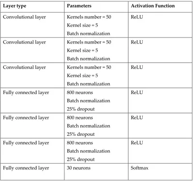
Table 1. The architecture of the network
Layer type Parameters Activation Function
Convolutional layer Kernels number = 50 Kernel size = 5 Batch normalization
ReLU
Convolutional layer Kernels number = 50 Kernel size = 5 Batch normalization
ReLU
Convolutional layer Kernels number = 50 Kernel size = 5 Batch normalization
ReLU
Fully connected layer 800 neurons
Batch normalization 25% dropout
ReLU
Fully connected layer 800 neurons
Batch normalization 25% dropout
ReLU
Fully connected layer 800 neurons
Batch normalization 25% dropout
ReLU
Fully connected layer 30 neurons Softmax
The Adam optimizer is used to train the network and the training rate is set to 0.01. The used accuracy metric is given by (9)
𝐴𝑐𝑐𝑢𝑟𝑎𝑐𝑦 =𝑇𝑃 𝑃 (9)
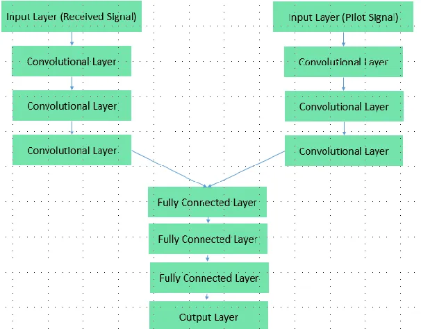
Three variants of the above architecture will be used. The first one seeks to simplify the problem and reduces its dimensionality by using several copies of the above network to estimate the location of each user alone, where the first network will be trained to estimate the location of the first user, the second network will be trained to estimate the location of the second user, and so on. The second variant will use an end-to-end approach where the performance of the whole system can be optimized. The above network will be used to estimate the locations of all users at the same time; however, several output layers are added to estimate the locations of different users. The third variant will introduce prior knowledge to the network by feeding the used pilot signal as an input to the network, where the above network is modified by adding one more input layer for the used pilot signal, followed by three convolutional layers, then the two branches are merged and the same fully connected layers are used. Fig. 1 shows the modified architecture. The performance of these three variants will be compared in the next section. Similar to the CS based approach, the output of the network for 10 signals will be combined.
Fig 1. A DL architecture where prior knowledge is incorporated
7. Results
Computer simulations were performed to evaluate the proposed approach. We consider the 2.4GHz industrial, scientific, and medical (ISM) band. The delay profile is represented by 30 samples, the Doppler resolution is represented by 30 samples. The proposed approaches will be used to localize users with random positions in the scene under different conditions. Training of the network took 12 hours on a standard Intel i3-4030U processor. First, we will compare the deep learning approach with existing methods, then the performance of the proposed architectures will be compared. After that, the performance of the deep learning approach is evaluated in the presence of multipath propagation. Then, the role of each parameter of the training set is evaluated, and finally, the effect of each parameter of the network is investigated.
A. Comparison with other methods in terms of accuracy and runtime
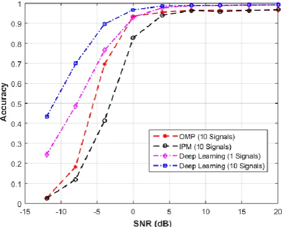
To compare the proposed deep learning approach with the compressive sensing approach described in section 5, 1000 Monte Carlo runs were performed to evaluate the compressive sensing approach under different SNR values where the locations of the users are generated randomly. Both the Orthogonal Matching Pursuit (OMP) [52] and the Interior Point Method (IPM) [53] were used to reconstruct the scene. Each reconstructed scene is the result of combining 10 signals. The same accuracy metric described in section 6 will be used to evaluate the CS approach. Fig. 2 shows the percentage of correctly detecting four users for the OMP and the IPM versus the first DL architecture which estimates the location of each object alone, the comparison is done for different SNR values, and when a different number of signals is combined. The DL based approach is showing a significant improvement in the accuracy, particularly for low SNR signals. This shows that the DL based approach has a higher ability to adapt to noisy environments where the conventional approaches are challenged.
B. Comparing with an end-to-end approach
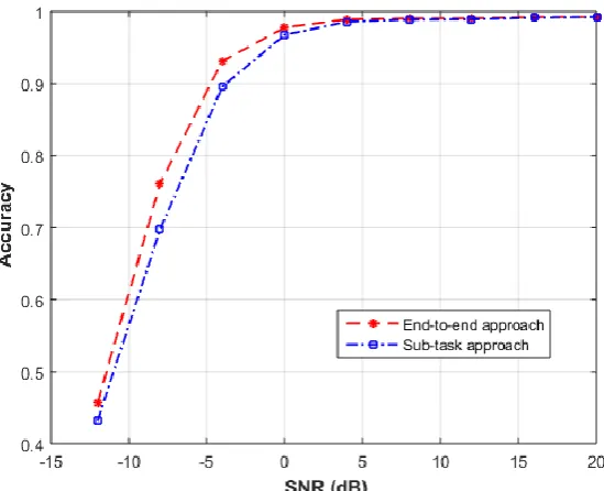
Two DL approaches will be compared, the first one tries to simplify the problem and reduces its dimensionality by estimating the location of each user alone as described in section 6. The second approach is an end-to-end approach where the locations of all users are estimated at the same time. The end-to-end approach has shown a better performance, which suggests that the gain from dividing this particular problem into simpler sub-tasks is lower than the gain from the overall optimization of the whole problem. Fig. 3 shows the probability of correctly detecting the users under different SNR values for the two approaches.
Fig 3. The probability of correctly detecting the users under different SNR values for the sub-task approach and the end-to-end approach.
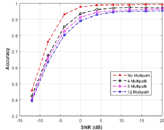
C. Comparing with an approach where prior knowledge is incorporating
Here we compare the end-to-end architecture with an architecture where prior knowledge is fed to the network. The used pilot signal is also used as an input to the network to see whether it will improve the performance of the network. The two approaches showed comparable results with a very small improvement of the prior knowledge approach, which means that there is no much gain from using additional information as an input to the network and the network is able to extract the needed information from the received signal. Fig. 4 shows the probability of correctly detecting the users under different SNR values for the two architectures.
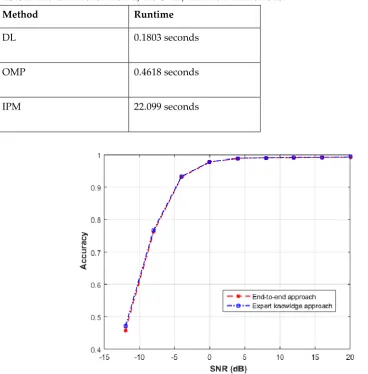
Table 2. The runtime for the DL, the OMP, and the IPM methods.
Method Runtime
DL 0.1803 seconds OMP 0.4618 seconds IPM 22.099 seconds
Fig 4. The probability of correctly detecting the users under different SNR values for the end-to-end approach and the approach when prior knowledge is incorporated.
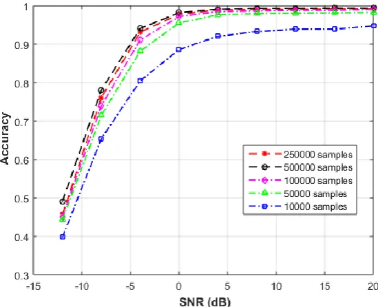
D. The effect of multipath
Fig 5. The probability of correctly detecting the users under different SNR values when 4, 8 and 12 multipath signals are used.
E. The effect of the SNR of the training set
To compare the effect of the SNR of the training samples, five sets will be tested. The first one contains signals with 20dB SNR, the second one contains signals with 0dB SNR, the third one contains signals with -12dB SNR, the fourth one contains signals with varying SNR starting from high SNR values to low SNR values i.e. from 20dB to -12dB, and the final set contains signals with varying SNR, however the signals here are sorted randomly. Fig. 6 shows the probability of correctly detecting the users under different SNR values for the five sets. Using the fourth and the fifth set have resulted in higher accuracy than the other sets, which means that the network should see examples from different SNR values. The -12dB set has shown higher accuracy at -12dB since there are more training samples at this SNR, however; the accuracy is much lower for other SNR values.
To investigate the effect of the number of the training examples on the performance of the proposed network, five sets with 10000, 50000, 100000, 250000, and 500000 training examples are compared. Fig. 7 shows the probability of correctly detecting the users under different SNR values for the five sets, the results show that the accuracy increases when a higher number of examples is used; however, the improvement becomes very small after 250000.
Fig 7. The probability of correctly detecting the users under different SNR values when different sizes of the training set are used.
G. The effect of different parameters of the network
Here we analyze the effect of different parameters on the performance of the network. First, we compare using a different number of neurons, then we compare using different number and sizes of kernels, and finally, we compare the role of dropout.
1. The effect of the number of neurons in each layer
Fig 8. The probability of correctly detecting the users under different SNR values when a different number of neurons is used.
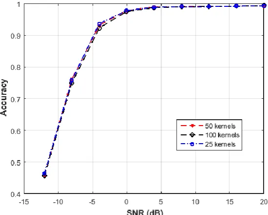
Then we compare changing the number of the kernels in the convolutional layers. 25, 50, and 100 kernels are compared. Fig. 9 shows the probability of correctly detecting the users under different SNR values for the three cases. Increasing the number of kernels has not resulted in increasing the accuracy where the three cases have shown comparable results. Fig. 10 shows the results for different sizes of the kernels, where kernels of size 9 are found to be slightly better in capturing useful features from the signal.
Fig 10. The probability of correctly detecting the users under different SNR values when different sizes of the kernels are used.
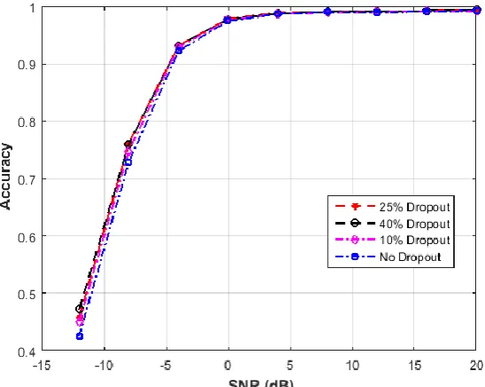
2. The effect of dropout
Here we compare the performance of the network for four cases, the first one is with no dropout, the second one is with 10% dropout, the third one is with 25% dropout, and the fourth one is with 40% dropout. Fig. 11 shows that increasing the dropout has resulted in more ability of the network to create useful features where 25% and 40% dropout are showing slightly higher accuracy.
8. Discussion
The proposed deep learning approach has shown higher performance with less runtime in comparison with the CS approach. The proposed approach has also shown a high ability to adapt to challenging environments. For the studied problem, using deep learning for each sub-task and hence reducing the curse of dimensionality has resulted in less accurate results in comparisons with the end-to-end approach where the performance of the whole system is optimized. Introducing prior knowledge by using the pilot signal as an input to the network has not resulted in much improvement in the accuracy, where the network seems to be able to extract the needed
information from the received signal. The proposed approach has also shown that it is relatively robust in multipath environments.
Increasing the number of examples in the training stage has resulted in higher accuracy; however, the improvement was very small after 250000. Using training examples from different SNR values has resulted in more accurate results in comparison of using the same SNR value for all the examples, whether that SNR is low or high. The results have also shown the role of different network parameters in improving the accuracy.
This work along with many other recent works have shown that deep learning has many potential applications in future signal processing, communication, and radar systems where conventional approaches are challenged. It represents a promising research direction that is still in its early stage. Some challenges still worth further investigations. Further research must be
conducted to propose deep learning architectures that best suit signal processing, communication, and radar systems.
9. Conclusions
This paper has presented a Wi-Fi based localization technique based on deep learning, where three different architectures were proposed. Simulation results demonstrated the significant improvement in the accuracy and in the runtime of the proposed approaches over existing approaches. The end-to-end architecture was found to be more accurate than the other two architectures. The proposed approach has also shown that it is relatively robust in multipath environments. Future work will investigate further improvement in the localization accuracy by building architectures that best suit localization systems.
Funding
This research received no external funding Conflicts of Interest:
The authors declare no conflict of interest.
References
1. Adib, F.; Kabelac, Z.; Katabi, D. Multi-person localization via RF body reflections. In Proceedings of the 12th USENIX Conference on Networked Systems Design and Implementation, Oakland USA, pp. 279-292, May 2015.
3. Chetty, K.; Smith, G.; Guo, H.; Woodbridge, K. Target detection in high clutter using passive bistatic WiFi radar. Proc. IEEE Radar Conf, Pasadena, CA, USA, pp. 1-5, May 2009.
4. Ender, J. A brief review of compressive sensing applied to radar. IEEE 14th international radar symposium, pp. 3-16, June 2013.
5. Hadi, MA.; Alshebeili, S.; Jamil, K.; El-Samie, FE. Compressive sensing applied to radar systems: an overview. Signal, Image and Video Processing, 2015, vol. 9, no. 1, pp. 25-39.
6. Anitori, L.; Maleki, A.; Otten, M.; Baraniuk, RG.; Hoogeboom, P. Design and analysis of compressed sensing radar detectors. IEEE Transactions on Signal Processing, 2013, vol. 61, no. 4, pp. 813-27. 7. Maechler, P.; Felber, N.; Kaeslin, H. Compressive sensing for wifi-based passive bistatic radar. Proc.
20th IEEE European Signal Processing Conf, Bucharest, Romania, pp. 1444-1448, August 2012. 8. Berger, C.R.; Zhou, S.; Willett, P. Signal Extraction Using Compressed Sensing for Passive Radar with
OFDM Signals. IEEE Int. Conf. Inf. Fusion, pp. 1-6, July 2008.
9. Khalili, A.; Soliman, A. A. Track before mitigate: aspect dependence-based tracking method for multipath mitigation. Electronics Letters, 2016, vol. 52, no. 4, pp. 316-317.
10. Khalili, A.; Soliman, A. A.; Asaduzzaman, M. Quantum particle filter: a multiple mode method for low delay abrupt pedestrian motion tracking. Electronics Letters, 2015, vol. 51, no. 16, pp. 1251-1253. 11. Krizhevsky, A.; Sutskever, I.; Hinton, G. Imagenet classification with deep convolutional neural
networks. In NIPS, 2012.
12. Zeiler, M. D.; Fergus, R. Visualizing and understanding convolutional neural networks. In ECCV, 2014. 13. Sermanet, P.; Eigen, D.; Zhang, X.; Mathieu, M.; Fergus, R.; LeCun, Y. Overfeat: Integrated recognition,
localization and detection using convolutional networks. In ICLR, 2014.
14. Deng, J.; Dong, W.; Socher, R.; Li, L.J.; Li, K.; Fei-Fei, L. Imagenet: A large-scale hierarchical image database. In Proc. CVPR, 2009.
15. O’Shea, T. J.; Hoydis, J. An introduction to deep learning for the physical layer. arXiv preprint arXiv:1702.00832, 2017.
16. Nachmani, E.; Be’ery, Y.; Burshtein, D. Learning to decode linear codes using deep learning. in Proc. Communication, Control, and Computing, pp. 341–346, 2016.
17. Nachmani, E.; Marciano, E.; Burshtein, D.; Be’ery, Y. RNN decoding of linear block codes. arXiv preprint arXiv:1702.07560, 2017.
18. Gruber, T.; Cammerer, S.; Hoydis, J.; Brink, S. On deep learning-based channel decoding. in Proc. of CISS, pp. 1–6, 2017.
19. Gruber, T.; Cammerer, S.; Hoydis, J.; Brink, S. Scaling deep learning-based decoding of polar codes via partitioning. arXiv preprint arXiv:1702.06901, 2017.
20. Nachmani, E.; Marciano, E.; Lugosch, L.; Gross, W. J.; Burshtein, D.; Beery, Y. Deep learning methods for improved decoding of linear codes. arXiv preprint arXiv:1706.07043, 2017.
21. Liang, F.; Shen, C.; Wu, F. An iterative BP-CNN architecture for channel decoding. arXiv preprint arXiv:1707. 05697, 2017.
22. Farsad, N.; Goldsmith, A. Detection algorithms for communication systems using deep learning. arXiv preprint arXiv:1705.08044, 2017.
23. Samuel, N.; Diskin, T.; Wiesel, A. Deep MIMO detection. arXiv preprint arXiv:1706.01151, 2017. 24. Ye, H.; Li, G. Y.; Juang. B.F. Power of deep learning for channel estimation and signal detection in
OFDM systems. arXiv preprint arXiv:1708.08514, 2017.
25. Neumann, D.; Wiese, T.; Utschick, W. Learning the MMSE channel estimator. arXiv preprint arXiv:1707.05674, 2017.
26. Wang, T.; Wen, C. K.; Wang, H.; Gao, F.; Jiang, T.; Jin, S. Deep learning for wireless physical layer: Opportunities and challenges. China Communications, 2017, vol. 14, no. 11, pp. 92-111.
27. Yonel, B.; Mason, E.; Yazıcı, B. Deep Learning for Passive Synthetic Aperture Radar. IEEE Journal of Selected Topics in Signal Processing, 2018, vol. 12, no. 1, pp. 90-103.
28. Mousavi, A.; Baraniuk, R. G. Baraniuk, Learning to invert: Signal recovery via deep convolutional networks. In Acoustics, Speech and Signal Processing (ICASSP), IEEE International Conference on, pp. 2272-2276, March 2017.
30. Kulkarni, K.; Lohit, S.; Turaga, P.; Kerviche, R.; Ashok, A. Reconnet: Non-iterative reconstruction of images from compressively sensed random measurements. Proc. IEEE Int. Conf. Comp. Vision, and Pattern Recognition, 2016.
31. Fang S. H.; Lin, T. N. “Indoor location system based on discriminant adaptive neural network in IEEE 802.11 environments,” IEEE Trans. Neural Network, 2008, vol. 19, no. 11, pp. 1973–1978.
32. Wang, X.; Gao, L.; Mao, S. CSI phase fingerprinting for indoor localization with a deep learning approach. IEEE Internet Things J, 2016, vol. 3, no. 6, pp. 1113–1123.
33. Wang, X.; Gao, L.; Mao, S.; Pandey, S. CSI-based fingerprinting for indoor localization: A deep learning approach. IEEE Trans. Veh. Technol, 2017, vol. 66, no. 1, pp. 763–776.
34. Wang, X.; Wang, X.; Mao, S. Cifi: Deep convolutional neural networks for indoor localization with 5 GHZ Wi-Fi. In Communications (ICC), 2017 IEEE International Conference on, pp. 1-6, May 2017. 35. Chen, H.; Zhang, Y.; Li, W.; Tao, X.; Zhang, P. ConFi: Convolutional Neural Networks Based Indoor
Wi-Fi Localization Using Channel State Information. IEEE Access, 2017, vol. 5, pp. 18066-18074. 36. IEEE standard for information technology, part 11: Wireless LAN medium access control (mac) and
physical layer (phy) specifications. June 2007.
37. Lecun, Y.; Bengio, Y.; Hinton, G. Deep learning. Nature, vol. 521, no. 7553, 2015. 38. Goodfellow, I.; Bengio, Y.; Courville, A. Deep learning. MIT press, 2016.
39. Hornik, K.; Stinchcombe, M.; White, H. Multilayer feedforward networks are universal approximators. Neural networks, 1989, vol. 2, no. 5, pp. 359–366.
40. Simonyan, K.; Zisserman, A. Very deep convolutional networks for large-scale image recognition. In ICLR, 2015.
41. Szegedy, C.; Liu, W.; Jia, Y.; Sermanet, P.; Reed, S.; Anguelov, D.; Erhan, D.; Vanhoucke, V.; Rabinovich, A. Going deeper with convolutions. In CVPR, 2015.
42. Bengio, Y.; Simard, P.; Frasconi, P. Learning long-term dependencies with gradient descent is difficult. IEEE Transactions on Neural Networks, 1994, vol. 5, no 2, pp. 157–166.
43. Glorot X.; Bengio, Y. Understanding the difficulty of training deep feedforward neural networks. In AISTATS, 2010.
44. He, K.; Zhang, X.; Ren, S.; Sun, J. Delving deep into rectifiers: Surpassing human-level performance on Imagenet classification. In ICCV, 2015.
45. Ioffe, S.; Szegedy, C. Batch normalization: Accelerating deep network training by reducing internal covariate shift. In ICML, 2015.
46. He, K.; and Sun, J. Convolutional neural networks at constrained time cost. In CVPR, 2015. 47. Srivastava, R. K.; Greff, K.; Schmidhuber, J. Highway networks. arXiv:1505.00387, 2015.
48. He, K.; Zhang, X.; Ren, S.; Sun, J. “Deep residual learning for image recognition,” In Proceedings of the IEEE conference on computer vision and pattern recognition, pp. 770-778, 2016.
49. Huang, G.; Liu, Z.; Weinberger, K. Q.; van der Maaten, L. Densely connected convolutional networks. In Proceedings of the IEEE conference on computer vision and pattern recognition, p. 3, July 2017. 50. Srivastava, N.; Hinton, G.; Krizhevsky, A.; Sutskever, I.; Salakhutdinov, R. Dropout: A simple way to
prevent neural networks from overfitting. The Journal of Machine Learning Research, vol. 15, no. 1, pp. 1929-1958.
51. George, D.; Huerta, E. Deep neural networks to enable real-time multimessenger astrophysics. arXiv preprint arXiv:1701.00008, 2016.
52. Tropp, J. A.; Gilbert, A. C. Signal Recovery from Random Measurements via Orthogonal Matching Pursuit. IEEE Trans. Inf. Theory, 2007, vol. 53, no. 12, pp. 4655 – 4666.
53. Dantzig, G.B.; Thapa, M.N. Linear Programming 2: Theory and Extensions. Springer-Verlag, 2003. 54. Jiang, H.; Cai, C.; Ma, X.; Yang, Y.; Liu, J. Smart Home based on WiFi Sensing: A Survey. IEEE Access,