Eleventh Floor, Menzies Building Monash University, Wellington Road CLAYTON Vic 3800 AUSTRALIA
Telephone: from overseas:
(03) 9905 2398, (03) 9905 5112 61 3 9905 2398 or 61 3 9905 5112
Fax:
(03) 9905 2426 61 3 9905 2426
e-mail: impact@buseco.monash.edu.au
Internet home page: http//www.monash.edu.au/policy/
Microeconomic Reform and Income
Distribution: The Case of Australian Ports
and Rail Freight Industries
by
G
EORGE
VERIKIOS
Centre of Policy Studies
Monash University
and
X
IAO
-
GUANG
ZHANG
Productivity Commission
Melbourne
General Paper No. G-230 July 2012
ISSN 1 031 9034 ISBN 978 1 921654 39 1
MICROECONOMIC REFORM AND INCOME DISTRIBUTION: THE
CASE OF AUSTRALIAN PORTS AND RAIL FREIGHT INDUSTRIES
George Verikios
Centre of Policy Studies, Monash University, Clayton, Victoria, Australia 3800.
Xiao-guang Zhang
Productivity Commission, Melbourne, Victoria, Australia 3000.
Abstract
We analyse structural changes in the Australian ports and rail freight industries during 1990s that were driven by microeconomic reform. We estimate the direct and indirect effects on household income groups of these industry changes by applying a computable general equilibrium model incorporating detailed household income and expenditure accounts, and microsimulation behaviour. The model contains both top-down and bottom-up linkages. The structural changes lead to a small increase in household welfare in most regions, with an overall increase of 0.18%. Income inequality is estimated to have decreased slightly by 0.02%.
JEL codes: C68, C69, D31, L92.
Keywords: computable general equilibrium, household income distribution, microeconomic reform, microsimulation, ports, rail freight.
Acknowledgements
Table of contents
1. Introduction 1
2. Microeconomic reform during the 1990s 2
2.1 Australian infrastructure industries and the Hilmer Reforms 2
2.2 Ports and the Hilmer Reforms 3
2.3 Rail freight and the Hilmer Reforms 4
3. Method: a CGE-microsimulation approach 5
3.1 The history of linked models 5
3.2 Analytical framework 6
3.3 The MMRF model with household accounts 7
3.3.1 A linear equation system 7
3.3.2 Behavioural equations 8
3.3.3 Household accounts 12
3.3.3.1 Theory 12
3.3.3.2 Data 15
3.4 Model closure 16
4. Calculating industry-specific changes 16
5 Results 18
5.1 Economy-wide effects 18
5.2 Household effects 21
6. Sensitivity analysis 22
7. Concluding remarks 24
Tables
1 Mapping between MMRF income sources and household income sources 15
2 Selected expenditure and income shares, national 16
3 Estimated changes in port and rail freight industry variables: 1989/90–1999/00
(percentage change) 19
4 Ports and rail freight industry effects due to changes in unit-output employment and relative output prices: 1989/90–1999/00 (percentage change) 20 5 Regional effects of changes in the ports and rail freight industries:
1989/90–1999/00 (percentage change) 21
6 Changes in household real income and inequality (percentage change) 22 7 Results of systematic sensitivity analysis: household real income and inequality
1. Introduction
In the early 1990s Australian governments introduced a series of microeconomic reform policies for infrastructure industries (e.g., ports, rail freight, telecommunications, electricity); Productivity Commission (PC) (2002) summarises these reforms. The reforms were part of the process produced by the Hilmer Report and, subsequently, the National Competition Reform Act
1995 and the Competition Principles Agreement between Australian governments.1 The Hilmer Report’s terms of reference focused on government businesses and regulations that had created protected enterprises: these had been a feature of industry policy in Australia for most of the 20th century. Hilmer argued for the introduction of competition policy in these areas in order to promote competition for the purpose of promoting community welfare, i.e., economic efficiency and other social goals (King and Maddock 1996). Thus, a major aim of the policy initiatives was to bring about market competition that, in turn, would lead to productivity improvements and attendant increases in real incomes, as well as better choice and services for consumers. Early in the reform process it was estimated that the reforms could increase national output by around 5.5% of its current value at the time (IC 1995). Since the initial introduction of the reforms, the affected industries have undergone significant structural changes that are observable in their cost structure and output prices. PC (2002) documents some of the infrastructure price changes in different Australian regions over 1990/91 to 2000/01.
As major service providers, changes in infrastructure industries can potentially have far-reaching impacts on other industries, businesses and households. Both PC (1999) and Madden (2000) noted that the competition policy reforms were regarded by many in the community as being responsible for the increased economic divide between capital cities and regional Australia. Related to this, there has also been natural community concern over the impact on income distribution of sectoral changes, in general, and infrastructure industry changes, in particular, viewed as a result of the microeconomic reforms.
There is a paucity of Australian studies that have analysed the distributional effects of the Hilmer reforms with only two notable exceptions. In PC (1996a), an input-output model and household survey data are used to estimate the effects on household expenditure of price reforms by government trading enterprises (GTEs) in the electricity industry and the water, sewerage and
1 Australia’s system of government is of federal form. Constitutional responsibilities are shared across the national
drainage services industry. In a companion paper (PC 1996b), a more sophisticated approach is adopted. A computable general equilibrium (CGE) model in conjunction with an income distribution model is used to analyse the effects of a specific set of reforms on the sources of household income. Each of these studies concentrates on only one side of the household budget, so the overall impact on household real income remains unclear. Moreover, input-output models, as applied in PC (1996a), do not capture effects generated from sectoral reallocation of resources that are arguably the most important effects of any policy change. As a result, the effects of a policy change derived from such a model may be misleading.
As a response to the shortcomings of previous studies, we conduct a more comprehensive analysis of the effects of industry changes on household income distribution: we focus on the ports and rail freight industries; these industries play an important role in the transport of domestic and international freight. We estimate the distributional effects of industry changes by integrating both sides of the household budget to capture the total (direct and indirect) effect on household real income. We do this by incorporating expenditure and income data on individual households within a multi-region CGE model. Within this framework we simulate the ports and rail freight-industry-specific changes during the 1990s to generate region-specific changes in the prices of goods and services, and productive factor returns and usage. Region-specific prices and other variables calculated by the CGE model are linked in a top-down manner to expenditure prices, employment and factor returns at the household level. In contrast, labour supply is determined at the household level and is linked to aggregate labour supply in a bottom-up manner. Our approach allows for a detailed analysis of changes in individual household expenditure and income. This represents a methodological advance on the few Australian studies that analyse the effects on income distribution of structural changes by incorporating both sides of the household budget. Further, it adds a regional dimension to the analysis that is lacking in previous studies.
2. Microeconomic reform during the 1990s2
2.1 Australian infrastructure industries and the Hilmer reforms
At the beginning of the 1990s Australian governments began an extensive process of microeconomic reform of Australian infrastructure industries; this included electricity, gas, water,
sewerage, urban passenger transport, port services, rail freight, telecommunications and postal services. The main objectives of these reforms were to increase competition and performance in these industries, and thus bring about higher living standards.
Prior to the commencement of the reform process almost all infrastructure industries were dominated by GTEs providing services with monopoly rights. Thus the reform process has been largely concerned with improving the performance of GTEs. With respect to GTEs, the reform process can be categorised into four broad areas: commercialisation; corporatisation; capital market disciplines; and competition policy.
1. Commercialisation. This involves GTEs taking a more market-driven approach to service
provision and pricing. To aid the commercialisation process, competitive tendering and contracting out of service provision have been introduced, community service obligations are now funded in a more direct and transparent way, and GTE regulatory functions have been transferred from GTEs to independent regulators.
2. Corporatisation. This focuses on making GTEs autonomous entities, within the public
sector, with commercially-oriented boards pursuing commercial objectives without ministerial interference. Financial and non-financial performance monitoring and reporting regimes were set up to measure and compare performance. Price regulation has also been largely transferred from ministerial control to independent regulators.
3. Capital market disciplines. Traditionally, GTEs were not required to earn a commercial rate
of return on their assets in the way that private sector firms must. This has now changed, with many governments requiring GTEs to either reduce negative rates of return or earn higher positive rates of return.
4. Competition policy. The implementation of the National Competition Policy Agreement has
focussed on removing existing entry barriers to infrastructure industries and thereby stimulating competition and increasing contestability. Increased competitive pressure is aimed at lowering prices and increasing service provision and quality.
2.2 Ports and the Hilmer reforms
authorities manage navigation channels and aids, berths, cargo storage areas and other wharf facilities.
The Hilmer reforms brought improvements to port governance arrangements that included: corporatisation; separation of commercial and regulatory functions; identification and costing of community service obligations (CSOs); and the introduction of dividend and tax-equivalent regimes. In many cases restructuring involved transforming port authorities into statutory bodies operating outside the departmental structure of government. There were also reforms to introduce contestability that mainly involved adoption of a landlord model of ownership and management (see IC 1993). Where the landlord model was adopted, it encouraged privatisation and contracting out of non-core activities. Many port authorities also sold their non-core assets. Pricing reforms involved shifting from charges based on the value of cargo handled to charges based on the costs of services rendered. Most governments also established independent price oversight for port charges.
2.3 Rail freight and the Hilmer reforms
Australian rail infrastructure is also important in the transport of domestic and international freight. In 1999/00, the Australian rail industry accounted for approximately one-third of the domestic freight task. Government and privately owned railways hauled over 134 billion net freight tonne kilometres (i.e., net freight tonnes hauled multiplied by the number of kilometres travelled). Rail authorities provide rail infrastructure and rolling stock.
Rail freight governance arrangements were reformed by commercialising GTEs and, in some cases, corporatising or privatising them. Other reforms included separating the management of rail stock from rolling stock. These reforms better clarified management objectives and responsibilities, identified and explicitly funded CSOs, and introduced stronger financial disciplines.
Australian Competition and Consumer Commission. These arrangements allowed the entry of a number of private operators, including interstate freight operators.
3. Method: a CGE-microsimulation approach
Our modelling approach links two separate analytical frameworks for the purpose of generating results at a high level of household detail without a complex CGE model that fully integrates individual households.
3.1 The history of linked models
As the inventor of microsimulation, it is not surprising that Orcutt (1967) was the first to describe a process for linking models that operate at differing levels of aggregation. He envisaged multiple models, each describing part of the economy, being linked as modules that together would describe the overall system. A succinct summary of alternative approaches to linking micro and macro models is provided by Bækgaard (1995) who identifies the following methods:
1. a top-down approach in which the micro model is adjusted to match an exogenous macro aggregate;
2. a bottom-up approach in which a change generated in the micro model is used to adjust the macro model;
3. a recursive linkage approach in which there is a two-way lagged interaction between models; and
4. an iterative approach in which the two models are solved simultaneously within each period.
A fifth approach proposed by Toder et al. (2000) involves the micro and macro models being solved separately over the full simulation period, with the models then calibrated and resolved until convergence is achieved. A further alternative is to build a model that inherently includes both a micro and macro dimension (Davies 2004). In principle, such a fully integrated model is preferred; in practice, most models in the literature take a recursive-linkage approach. This reflects the practical difficulties of including both dimensions within the one model.
is provided by Meagher and Agrawal (1986) in which output from a CGE model was used to reweight the 1981–82 National Income and Housing Survey. Their approach was updated by Dixon et al. (1996), who also foreshadowed an iterative linking of a CGE model to either a static or dynamic microsimulation model. In related work, Polette and Robinson (1997) used the top-down approach to link an aggregated version of the MONASH dynamic CGE model to a microsimulation model of the Australian income support system.
Of the two Australian studies that have analysed the distributional effects of the Hilmer reforms, PC (1996b) follows the pioneering work (in the Australian context) of Meagher and Agrawal (1986) by using a CGE model in conjunction with an income distribution model to analyse the effects of some of the Hilmer reforms on the sources of household income. PC (1996a) applies an input-output model and household survey data to estimate the effects on household expenditure of price reforms by GTEs in the electricity industry and the water, sewerage and drainage services industry. But input-output models are inappropriate for analysing distributional effects as they assume all prices are fixed whereas, in reality, any reallocation in resources across sectors due to structural change will alter factor prices and incomes. Further, both PC studies concentrate on only one side of the household budget so the overall impact on household real income is unclear.
3.2 Analytical framework
Most of the Australian studies mentioned above have focused on linking a CGE model to a detailed microsimulation model of household income. Thus, they have mostly ignored the differences in expenditure patterns across households and their effect on estimates of distributional effects. Further, none of these studies employed a bottom-up regional model of Australia that can capture region-specific changes and thus derive region-specific changes in commodity and factor prices, and region-specific changes in resource allocation across industries. Allowing for region-specific changes in analysing structural change in Australian infrastructure industries due to the microeconomic reform process is important, as the reform process did not proceed at an even pace and was not of a similar nature across the Australian regions. This is a function of the reform process being the responsibility of regional (state and territory) governments, rather than the national government.3
As a response to the shortcomings of previous Australian studies, we develop a more comprehensive framework by (i) integrating both sides of the household budget to capture the effects on household real income, and (ii) employing a regional model to generate region-specific changes in commodity prices, factor prices and factor usage. A comparative-static multi-region CGE model – the Monash Multi-Region Forecasting (MMRF) model (Naqvi and Peter 1996) – is modified by incorporating individual household income and expenditure accounts. The household accounts are linked to the CGE accounts by which they are updated in a mostly top-down manner. Importantly, though, labour supply by occupation is determined at the household level in each region. Labour supply is then linked in a bottom-up manner to the core of the CGE model. In terms of the four approaches identified by Bækgaard (1995), our approach is a combination of approaches (1) and (2).
3.3 The MMRF model with household accounts
The MMRF model represents the supply and demand side of commodity and factor markets in the eight Australian regions. Each region contains five representative agents – producers, physical capital investors, households, governments and foreigners. There are 54 producers in each region, each producing one commodity. Commodities are traded between regions and are also exported. There is a single representative household in each region that owns all factors of production and thus receives all factor income (net of taxes): households can either spend or save their income. Saving contributes to the financing of domestic investment. There are nine government sectors (eight regional and one national). Foreigners supply imports to each region at fixed c.i.f. prices, and demand commodities (exports) from each region at variable f.o.b. prices.
3.3.1 A linear equation system
MMRF is represented by equations specifying behavioural and definitional relationships. There are m such relationships involving a total of p variables and these can be compactly written in matrix form as
Av=0, (1)
where A is an m×p matrix of coefficients, v is a p×1 vector of percentage changes in model variables and 0 is the p×1 null vector. Of the p variables, e are exogenous (e.g., input-output
endogenous variables. Many of the functions underlying (1) are highly nonlinear. Writing the equation system like (1) allows us to avoid finding the explicit forms for the nonlinear functions and we can therefore write percentage changes in the
(
p e−)
variables as linear functions of the percentage changes in the e variables. To do this, we rearrange (1) as1
n x A A− =
-n x , (2)
where n and x are vectors of percentage changes in endogenous and exogenous variables, and An and Ax are matrices formed by selecting columns of A corresponding to n and x. If An is square and nonsingular, we can compute percentage changes in the endogenous variables as in (2). Computing solutions to an economic model using (2) and assuming the coefficients of the A
matrices are constant is the method pioneered by Johansen (1960).
Equations (1) represent the percentage-change forms of the nonlinear functions underlying the model; these forms are derived by total differentiation. Thus, (1) is an approximation based on marginal changes in the independent variables. So (2) only provides an approximate solution to the endogenous variables n; for marginal changes in x the approximation is accurate but for
discrete changes in x the approximation will be inaccurate. The problem of accurately
calculating n for large changes in x is addressed by allowing the coefficients of the A matrices to
be nonconstant; this is done by breaking the change in x into i equal percentage changes. The
multistep solution procedure requires that there are
( )
i−1 intermediate values of the underlying (levels) values of n, i.e., N. The intermediate values of N are obtained by successively updatingthe values of N after each of the i steps is applied. Once the values of N are updated for any
given step, the coefficients of the A matrices in (2) are recomputed before (2) is solved again.4 Below we present the important behavioural equations for producers in the model.
3.3.2 Behavioural equations
Representative firms are assumed to treat the three factors of production (agricultural land, eight labour types and physical capital) as variable and take factor prices as given in minimising
4 The model is implemented and solved using the multistep algorithms available in the GEMPACK economic
costs. Demands for primary factors are modelled using nested production functions consisting of three levels. At the top level, the j (=1,…,54) firms in the r (=1,..,8) regions decide on the (percentage change in) demand for the primary factor composite (i.e., an aggregate of land, labour and capital) qfjrF using Leontief production technology:
F
jr jr jr
qf =qf +af ; (3) where qf is (the percentage change in) the jr
( )
j r -th industry’s activity level, and , af is jr technical change augmenting the use of all production inputs. By applying Leontief production technology, we are assuming that firms’ use of the primary factor composite is a fixed share of output, reflecting the idea that the value added share of output is invariant to changes in relative prices and reflects characteristics intrinsic to the production of each good.At the second level, firms decide on their demand for the i (=3) factors of production, qfijrF. All industries apply CES (constant elasticities of substitution) production functions:
(
)
F F F F F F F
ijr jr ijr jr ijr ijr jr
qf =qf +af −σf pf +af −pf ; (4) where σfjrF
(
=0.5)
is the elasticity of factor substitution,F ijr
af is factor i-augmenting technical change, and pfijrF
( )
Fjr
pf is the individual (average) price of primary factors. For i = Capital, (4) represents stocks of capital used by each industry. These stocks represent past investments net of depreciation. Any investment that occurs from perturbing the model will add to existing stocks if it exceeds depreciation.
At level 3, firms decide on their use of the m (=8) labour types (occupations) qfmjrL using CES production technology,
(
)
L F L L L
mjr ijr mr mjr jr
qf =qf −σf pf −pf , i=labour (5)
where σfL
(
=0.35)
is the CES between any pair of labour types, and pfmjrL( )
L jrpf is the individual (average) wage rate paid to the m-th labour type.
We add a supply function for labour type m supplied by household c in region r, c mr ls , c c c
mr mr
ls =β rw , (6)
and
c c
mr mr r
rw =w −p , (7)
where wmr is the average post-income-tax wage paid to the
( )
m r, -th labour type. Thus, (7) assumes that all households supplying the( )
m r, -th labour type are paid a common wage rate.c r
p is the household-specific consumer price index in region r and is defined in Section 3.3.3. So the household supply of each labour type is a positive function of the real wage, c
mr
rw , and βc , the household labour supply elasticity. βc
is set at 0.15 reflecting econometric evidence on labour supply in Australia (Kalb 1997).
The initial labour market equilibrium includes unemployment in each region. Changes in the equilibrium are determined by imposing a relation between the pre-income-tax real wage
*
mr
rw and employment lmr of the form,
*
mr mr
rw =γl , (8)
and
* *
mr mr r
rw =w −p , (9)
54
1
L L mr j mjr mjr
l =
∑
= S qf . (10)Equation (9) defines rw as the pre-income-tax wage rate deflated by the regional consumer mr*
price index; equation (10) defines employment in occupation m in region r as the share-weighted sum of employment by occupation across all industries.
γ
in (8) represents the employment elasticity of the real wage, i.e., the responsiveness of the real wage to changes in employment. In any perturbation of the model,γ
determines the degree to which increases (decreases) in the demand for the( )
m r, -th labour type will be reflected in higher (lower) employment or the real wage. The value γ varies depending on whether the real wage is rising or falling. For rw*mr ≥0,grow faster than employment.5 For *
0 mr
rw < , γ equals 0.5 making real wages stickier downwards than upwards, which is also consistent with features of the Australian labour market whereby there is effectively a minimum wage for all jobs in all industries. Equations (6) and (8) together determine the endogenous unemployment rate for the
( )
m r, -th labour type.Firms are also assumed to be able to vary the k (=1,…,54) intermediate inputs they use in production, the prices of which they also take as given in minimising costs. In combining intermediate inputs, all firms are assumed to use nested production functions. At level 1, all firms decide on their use of the intermediate input composite qfjrI using Leontief production technology;
I
kjr jr jr
qf =qf +af . (11)
At level 2, firms decide on their use of the k intermediate input composites from domestic region r qfkjrI using CES production technology,
(
)
I I I I I
kjr kjr k kjr kjr
qfd =qf −σf pfd −pf , (12)
where I k f
σ is the CES for domestic intermediate input composites, and I
( )
I kjr kjrpfd pf is the individual (average) price of domestic intermediate input composites. The values for I
k f
σ range between 1 and 2 for most goods; the exceptions are low-value manufactured goods (e.g., textiles, clothing and footwear) that are set at 3 or more.
At level 3, firms decide on their use of individual intermediate inputs by source s (eight domestic sources and one foreign source qfskjsrI ) also using CES production technology,
(
)
I I I I I
kjsr kjr k kjsr kjr
qfs =qfd −σfd pfs −pfd , s=domestic; (13)
(
)
I I I I I
kjsr kjr k kjsr kjr
qfs =qf −σ f pfs −pf , s=foreign; (14)
where I
k fd
σ is the CES between any pair of individual intermediate inputs from domestic sources, and I
kjsr
pfs is the price of the k-th intermediate input from region s used by firm j in
region r. The values for I k fd
σ range from 2.5 for high-value manufactured goods (e.g., scientific
5 Equation (8) is also consistent with the wage curve idea of Blanchflower and Oswald (1995) that suggests an
equipment), 8 for primary goods (e.g., agriculture), and 10 or more for low-value manufactured goods.
We define average technical change for a given industry as the share-weighted sum of the technical change terms already defined,
F F jr jr ijr ijr
a =af +S af . (15)
where S is the cost share of the i-th factor. ijrF
All firms are assumed to operate in perfectly competitive markets and so we impose a zero-pure-profits condition that is expressed as equating revenues with costs;
(
)
(
)
3 54
1 1
F F F I I I
jr jr i ijr ijr ijr k kjr kjr kjr jr
pf +qf =
∑
= S pf +qf +∑
= S pf +qf +a . (16) Equation (16) forces revenue for the firm(
pfjr+qfjr)
to move with the sum of the costs of the ifactor inputs
(
pfijrF +qfijrF)
and k intermediate inputs(
)
I I kjr kjrpf +qf , weighted by cost shares (the
Ss). Equation (16) determines the
( )
j r -th industry’s activity level ,( )
qfjr . Commodity prices are determined by a market-clearing condition for each commodity.To facilitate the imposition of changes in the relative price of ports and rail freight, we add the equation
jr jr r
rp = pf −cpi , j∈
{
ports, rail freight}
, (17) where cpi is the consumer price index in region r. rIn order to impose exogenous changes in employment per unit of output we add the equation
F jr ijr jr
qfl =qf −qf , i=labour. (18)
3.3.3 Household accounts
The household accounts we add to MMRF represent the distribution of real incomes across households in eight Australian regions.
3.3.3.1 Theory
CV and EV apply a ‘money-utility’ concept rather than utility itself. A modified version of the CV is based on redefining real income as constant purchasing power. Applying this concept to measure changes in real income means there is no need to make any specific assumptions about consumer preferences or utility functions.
The computation of CV normally assumes unchanging household income and, therefore, emphasises only the role of each household’s consumption patterns in determining the welfare impact of a price change. But in a general equilibrium framework household income is not constant, so we extend the modified CV to account for changing income. For a household, real income can then be defined as nominal factor earnings and transfers received from different sources deflated by a household-specific consumer price index (HCPI). Then, the first-order approximation to the percentage change in the c-th household’s CV, relative to the initial consumption bundle and factor ownership, can be expressed as
(
)
c c c
cv = − i −p , (19)
where i and c p are the percentage changes in income and the HCPI for household c. c p is the c
average percentage change in the prices of the n goods consumed p weighted by expenditure n
shares S : nc
c c
n n n
p =
∑
S p . (20)Differences in the sources of income c
i for the c-th household can be expressed as
c c
g g g
i =
∑
S i , (21)where S is the share of income source g in total household income, and gc i is the percentage g
change in the price of income source g. The elements of the set of income sources g (=33) are
listed in Table 1.
The income side of our modified CV is the amount of money that would encourage households to supply the same amount of factors as prior to any price change. But the general equilibrium effects of industry changes will lead to changes in factor supply and employment, as well as factor returns. To account for such changes, we redefine c
i as
(
)
c c
g g g g
where q is the percentage change in the demand (or employment) of income source g. Thus, g our modified CV assesses the impact of a policy change on a given household or household group via the computation of the change in real income.
In computing real household income changes, price and quantity changes are mapped from less detailed MMRF variables to more detailed variables in the household accounts. Commodity prices are mapped as 54
1
c
nr k kn kr
p =
∑
=CM p , where a regional subscript has been added and CM knis a (0,1)-integer matrix mapping from MMRF commodities to more detailed household expenditure data. The household-specific consumer price index in region r p is then a share-rc
weighted sum of p across all commodities. nrc
Wages for the m (=8) occupations are mapped as imrc =w*mr+lmr, i.e., the wage rate times the quantity of labour of
( )
m r -th occupation. The s (=12) non-labour income sources are , mapped as isrc = pfrNL+qfrNL, whereNL r
pf and qfrNL are the average rental rate and quantity of capital and land in region r.
For income source g = unemployment benefits, igrc =cpi+pbr+unemr, where cpi is the
national consumer price index, pbr is the federal government’s personal benefits receipts rate, and unem is the number of unemployed in region r. For other government benefits, income is r
mapped as igrc =cpi+pbr+popr, where pop is population in region r. Note that cpi is the r
numeraire, and pbr and pop are assumed to be exogenous. Thus, government benefit r payments will only be affected via changes in the number of unemployed. Household income from all income sources is then 33
1
c c c
r g gr gr
i =
∑
=S i , where S is the share of income source g in grc total income for household c in region r. Household disposable income di is determined as grc(
)
c c c c c r r r r r
di =SI i −ST i +tr , where tr is the income tax rate, and SI is the share of total income in rc disposable income and ST is the share of income taxes in disposable income. Real household rc disposable income c
r
rdi is then
c c c r r r
3.3.3.2 Data
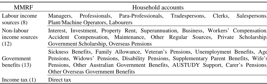
The household accounts are based on unit-record household survey data taken from the 1993/94 Household Expenditure Survey (HES93) (ABS 1994). The survey contains detailed information on household consumption patterns and income sources of 8,389 sample households across the eight Australian states and territories. On the income side, the HES93 lists private income sources, such as wages and salaries from eight occupations and non-wage income from investment or business sources, as well as various government transfer payments, such as family allowances, unemployment benefits and age pensions (see Table 1). It also contains expenditure data on more than 700 goods and services.
Table 1. Mapping between MMRF income sources and household income sources
MMRF Household accounts
Labour income sources (8)
Managers, Professionals, Para-Professionals, Tradespersons, Clerks, Salespersons, Plant/Machine Operators, Labourers
Non-labour income sources (12)
Interest, Investment, Property Rent, Superannuation, Business, Workers’ Compensation, Accident Compensation, Maintenance, Other Regular Sources, Private Scholarship, Government Scholarship, Overseas Pensions
Government benefits (13)
Sickness Benefits, Family Allowance, Veteran’s Pensions, Unemployment Benefits, Age Pensions, Widows’ Pensions, Disability Pensions, Supplementary Parent Benefits, Wife’s Pensions, Other Australian Government Benefits, AUSTUDY Support, Carer’s Pensions, Other Overseas Government Benefits
Income tax (1) Direct tax
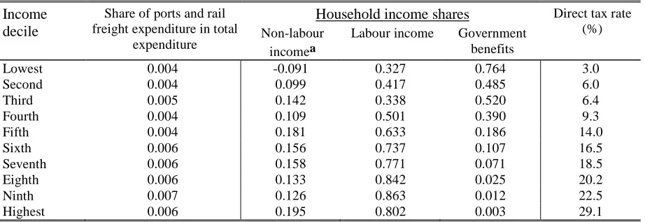
Table 2. Selected expenditure and income shares, national
Income decile
Share of ports and rail freight expenditure in total
expenditure
Household income shares Direct tax rate (%) Non-labour
incomea
Labour income Government benefits
Lowest 0.004 -0.091 0.327 0.764 3.0
Second 0.004 0.099 0.417 0.485 6.0
Third 0.005 0.142 0.338 0.520 6.4
Fourth 0.004 0.109 0.501 0.390 9.3
Fifth 0.004 0.181 0.633 0.186 14.0
Sixth 0.006 0.156 0.737 0.107 16.5
Seventh 0.006 0.158 0.771 0.071 18.5
Eighth 0.006 0.133 0.842 0.025 20.2
Ninth 0.007 0.126 0.863 0.012 22.5
Highest 0.006 0.195 0.802 0.003 29.1
Source: MMRF household accounts.
a Non-labour income sources are defined in Table 1. They are based on taxable income; thus, they include losses from business and property income. Such losses dominate non-labour income for the lowest income decile as a whole.
3.4 Model closure
The model contains m equations and p variables where m < p, so to close the model e (= p – m) variables must be set as exogenous. The exogenous variables are chosen so as to
approximately simulate a long-run environment. Thus, technical change, indirect tax rates, and industry depreciation rates are exogenous. To capture the overall scarcity of land, we also fix industry land usage. As this study is concerned with the reallocation of existing factors rather than growth effects, the national supply of capital is fixed. This means that any excess demands for capital at initial prices (due to industry changes) are partly reflected in rental price changes and partly reflected in the reallocation of capital across regions and sectors: capital moves between industries and across regions to maximise its rate of return. The national consumer price index is the numeraire, thus nominal price changes are measured relative to this composite price.
4. Calculating industry-specific changes
isolate all changes that are specific to these industries. To estimate such changes, the observed changes in these industries need to be adjusted to remove the effects of external factors. If complete information on changes in the quantities of industry inputs and outputs was available, these changes could be imposed directly as shocks in the model to generate the requisite equilibrium prices and quantities for ports and rail freight, as well as other commodities and primary factors. But information is only available on two industry variables: employment and output prices.
The observed changes in industry gross employment contain an expansionary effect caused by economy-wide output growth (due to changes in productivity, tastes and preferences, technology, etc.), which may be unrelated to industry-specific changes. To remove this effect, employment per unit of output is used to simulate the change in the ports and rail freight industries’ employment. Employment per unit of output is calculated as observed gross employment divided by the quantity of output. For ports, output is cargo handled annually in mass tonnes; for rail freight, output is net freight tonne kilometres.
In imposing the changes in employment per unit of output on the model, this typically endogenous variable, qfl in equation (18), must bet set as exogenous. This is accommodated by jt
setting labour-augmenting technical change as endogenous, afijrF
(
i=labour)
in equation (4). This implicitly assumes that any change in unit-output employment can be attributed to a change in industry-specific labour productivity.In calculating the price shocks, we want to remove the effects of factors not specific to the ports and rail freight industries, e.g., inflation, income growth, population expansion, etc. The impacts of these external effects on the price of ports and rail freight can be removed, to a large extent, by calculating a ‘real price index’, i.e., the observed market price divided by the consumer price index (CPI). If the CPI is taken as a proxy for the price index of all goods and services, the real price of ports and rail freight can be conveniently interpreted as a relative price. Any deviation of the real price from the CPI can then be interpreted as indicating changes caused purely by industry-specific factors. The real price of ports and rail freight is typically an endogenous variable in the model, rp in equation (17). To impose the price change in MMRF, jr we set it as exogenous and all-input-augmenting technical change is set as endogenous, af in jr
Changes in these industries are also likely to affect government revenue. To neutralise the effect of changes in government revenue in the analysis, we fix the federal budget deficit and endogenise the income tax rate. We also fix the budget deficit for all state governments and endogenise their payroll tax rates. This assumes that for a given level of public expenditure, any increased tax revenue due to industry changes will be automatically returned to households though a decrease in their income tax rates, and higher pre-tax wage rates due to lower payroll tax rates on firms.
5. Results 5.1 Economy-wide effects
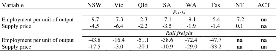
In this section the estimated changes in the real price and employment per unit of output in the ports and rail freight industries are applied to MMRF to project the effects of these changes on the wider economy. The changes are estimated from published statistics and are reported in Table 3.6 We see that employment per unit of output decreased slightly for the ports industry, from a maximum of -9.7% in NSW and a minimum of -2.3% in Queensland. Much larger changes in employment per unit of output were observed for the rail freight industry: this ranged from -72% in WA to -16% in Victoria. The changes in real prices were generally negative and were also smaller for the ports industry; price changes ranged from 0.1% (NT) to -6.4% (Victoria) for the ports industry; price changes ranged from -3% (Victoria) to -33% (Tasmania) for the rail freight industry.
6 MMRF does not contain separate ports and rail freight industries. These industries form part of the larger Services
Table 3. Estimated changes in port and rail freight industry variables: 1989/90–1999/00 (percentage change)
Variable NSW Vic Qld SA WA Tas NT ACT
Ports
Employment per unit of output -9.7 -7.3 -2.3 -7.1 -9.1 -5.4 -7.2 na
Supply price -4.5 -6.4 -2.2 -3.5 -1.9 -1.4 0.1 na
Rail freight
Employment per unit of output -43.8 -16.4 -51.1 -38.6 -72.4 -47.7 na na
Supply price -17.5 -3.0 -20.1 -10.9 -29.0 -33.2 na na
Source: SCNPMGTE (1995, 1996, 1998); PC (2002); ANRC (1991, 1993, 1994, 1995, 1997); FreightCorp (1998, 1999, 2000);
Queensland Rail (1998, 1999, 2000); Westrail (1998, 2000). See Chapter 4 of Verikios and Zhang (2005) for further details.
A CGE model captures both the direct and indirect effects of a given shock to the economy. The major determinant of the direct effects of changes in the ports and rail freight industries is their combined importance in the economy as a whole. Our model data indicates that value-added for these industries made up around 2.2% of national value-value-added. This varies from less than 1% in the Australian Capital Territory (ACT) to 3.1% in South Australia. Port and rail freight services are predominately used to transfer goods between industries and to export points. This means they are typically used as a margin input to production. Thus, changes in these industries will mainly affect household incomes indirectly, by affecting returns to primary factors and the prices of final goods and services.
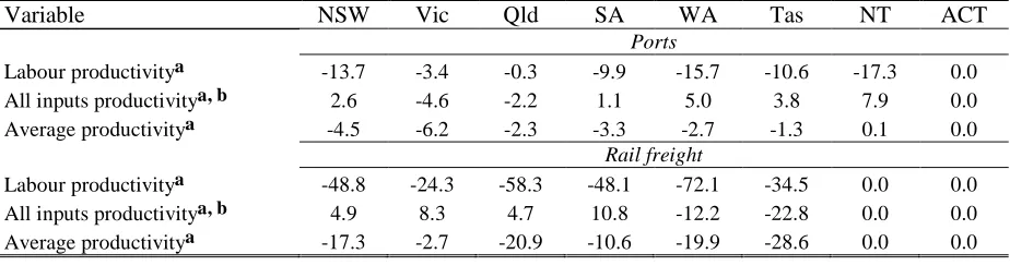
The results of applying the estimated changes in employment and prices to MMRF are reported in Table 4. The estimated changes in unit-output employment will determine the changes in labour productivity.7 The estimated changes in supply prices will determine the change in the productivity of all inputs, i.e., all primary factors and intermediate inputs. The change in labour- and all-input augmenting technical change is summed to give average technical change, a in equation (15). This change is closely related to the change in the supply price for jr
the industry. Average productivity is projected to improve in all regions where industry changes were observed except the Northern Territory (NT). As expected, larger improvements are estimated for the rail freight industry. The pattern of productivity changes across regions largely mimic the pattern of changes in real prices and unit-output employment reported in Table 3.
7 When referring to productivity changes in discussing model results, we are referring to the model equivalent of
Table 4. Ports and rail freight industry effects due to changes in unit-output employment and relative output prices: 1989/90–1999/00 (percentage change)
Variable NSW Vic Qld SA WA Tas NT ACT
Ports
Labour productivitya -13.7 -3.4 -0.3 -9.9 -15.7 -10.6 -17.3 0.0
All inputs productivitya, b 2.6 -4.6 -2.2 1.1 5.0 3.8 7.9 0.0
Average productivitya -4.5 -6.2 -2.3 -3.3 -2.7 -1.3 0.1 0.0
Rail freight
Labour productivitya -48.8 -24.3 -58.3 -48.1 -72.1 -34.5 0.0 0.0
All inputs productivitya, b 4.9 8.3 4.7 10.8 -12.2 -22.8 0.0 0.0
Average productivitya -17.3 -2.7 -20.9 -10.6 -19.9 -28.6 0.0 0.0
Source: MMRF simulation.
a This is the input requirement per unit of output; thus, a negative sign signifies an improvement. b This relates to all primary factors and intermediate inputs.
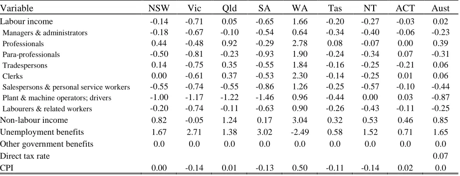
The national changes in relative occupational incomes (Table 5) indicate which occupations are favoured by the industry changes; these show large relative reductions for Plant and machine operators, drivers, Salespersons and personal service workers, and Para-professionals. This is
because around half of all wage payments in the ports & rail freight industries are made to these three occupations. Thus, when significant labour shedding occurs in these industries it is primarily Plant and machine operators, drivers, Salespersons and personal service workers, and Para-professionals who are affected, and consequently the wage rates for these occupations must
fall for them to be reemployed in other industries. Occupations that are least used in the ports and rail freight industries and most used in expanding industries experience the largest increases in relative incomes, e.g., Professionals.
Table 5. Regional effects of changes in the ports and rail freight industries: 1989/90– 1999/00 (percentage change)
Variable NSW Vic Qld SA WA Tas NT ACT Aust
Labour income -0.14 -0.71 0.05 -0.65 1.66 -0.20 -0.27 -0.03 0.02 Managers & administrators -0.18 -0.67 -0.10 -0.54 0.64 -0.34 -0.40 -0.06 -0.23 Professionals 0.44 -0.48 0.92 -0.29 2.78 0.08 -0.07 0.00 0.39 Para-professionals -0.50 -0.81 -0.23 -0.93 1.90 -0.24 -0.34 0.07 -0.31 Tradespersons 0.14 -0.75 0.35 -0.55 1.84 -0.16 -0.25 -0.21 0.06 Clerks 0.00 -0.61 0.37 -0.53 2.30 -0.14 -0.25 0.01 0.06 Salespersons & personal service workers -0.55 -0.74 -0.55 -0.86 1.26 -0.25 -0.57 -0.10 -0.44 Plant & machine operators; drivers -1.00 -1.17 -1.22 -1.46 0.96 -0.44 0.00 0.03 -0.87 Labourers & related workers -0.20 -0.74 -0.11 -0.63 0.90 -0.26 -0.43 -0.11 -0.25 Non-labour income 0.82 -0.05 1.24 0.17 3.04 0.32 0.53 0.46 0.85 Unemployment benefits 1.67 2.71 1.38 3.02 -2.49 0.58 1.52 0.71 1.65 Other government benefits 0.0 0.0 0.0 0.0 0.0 0.0 0.0 0.0 0.0
Direct tax rate 0.07
CPI 0.00 -0.14 0.01 -0.13 0.50 -0.11 -0.14 0.02 0.0
Source: MMRF simulation.
Non-labour income also increases nationally reflecting increased demand for capital and land. The relative changes in non-labour income across regions reflect the pattern of movements in labour income across regions. Unemployment benefits fall in regions that experience higher employment (WA) and rise in regions that experience lower employment (all other regions).
Besides the changes in primary factor incomes, the direct tax rate will also affect household post-tax income. With the assumption of a fixed federal budget deficit and an endogenous direct tax rate, changes in the direct tax rate are driven by the effect of changes in the ports and rail freight industries on total tax revenue. Changes in total tax revenue are driven by the effect of the industry changes on the level of economic activity. While productivity improves in most regions, there is a small contractionary effect in net terms on economic activity nationally; thus the direct tax rate rises slightly (0.07%).
5.2 Household effects
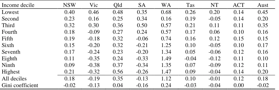
Table 6. Changes in household real income and inequality (percentage change)
Income decile NSW Vic Qld SA WA Tas NT ACT Aust
Lowest 0.40 0.46 0.48 0.35 0.68 0.26 0.20 0.14 0.45
Second 0.23 0.16 0.25 0.34 0.16 0.19 -0.05 0.14 0.20
Third 0.32 0.30 0.36 0.50 0.57 0.21 0.11 0.11 0.35
Fourth 0.18 -0.09 0.27 0.24 0.57 0.17 0.06 0.10 0.16
Fifth 0.19 -0.18 0.32 -0.06 0.74 0.16 0.12 0.15 0.15
Sixth 0.15 -0.20 0.32 -0.21 1.25 0.10 -0.05 0.10 0.17
Seventh 0.17 -0.24 0.23 -0.20 1.34 0.05 -0.06 0.12 0.16
Eighth 0.11 -0.35 0.24 -0.33 1.49 -0.04 -0.12 0.11 0.10
Ninth 0.09 -0.38 0.37 -0.34 1.35 0.07 -0.09 0.12 0.11
Highest 0.21 -0.32 0.56 -0.26 1.47 0.09 -0.04 0.14 0.20
All deciles 0.18 -0.19 0.35 -0.13 1.12 0.10 -0.01 0.12 0.18
Gini coefficient -0.02 -0.13 0.04 -0.16 0.24 -0.03 -0.04 0.00 -0.02
Source: MMRF simulation.
Decomposing the change in real household income by decile into the change in nominal disposable income and the change in the price index, indicates that nationally the price changes are around -0.1% for all deciles. Thus, the differences in real household income across deciles are mainly a reflection of the differences in nominal disposable income across deciles: the latter show relatively larger income gains for lower income deciles. The relatively larger income gains for lower income deciles are mainly due to a rise in labour income and unemployment benefits. Most upper income deciles receive relatively smaller increases in labour income (or experience small falls in labour income), and gain little from the rise in unemployment benefits as the unemployed are found mainly in lower income deciles.
6. Sensitivity analysis
standard deviations will be good approximations to the true means and standard deviations under certain conditions (Arndt and Pearson 1996).8
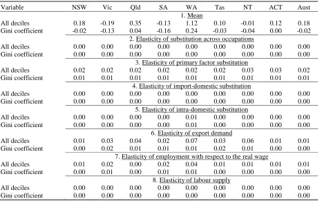
Table 7. Results of systematic sensitivity analysis: household real income and inequality (percentage change)
Variable NSW Vic Qld SA WA Tas NT ACT Aust
1. Mean
All deciles 0.18 -0.19 0.35 -0.13 1.12 0.10 -0.01 0.12 0.18
Gini coefficient -0.02 -0.13 0.04 -0.16 0.24 -0.03 -0.04 0.00 -0.02
2. Elasticity of substitution across occupations
All deciles 0.00 0.00 0.00 0.00 0.00 0.00 0.00 0.00 0.00
Gini coefficient 0.00 0.00 0.00 0.00 0.00 0.00 0.00 0.00 0.00
3. Elasticity of primary factor substitution
All deciles 0.02 0.02 0.02 0.02 0.02 0.02 0.03 0.03 0.02
Gini coefficient 0.01 0.01 0.01 0.01 0.01 0.01 0.01 0.01 0.01
4. Elasticity of import-domestic substitution
All deciles 0.00 0.00 0.00 0.00 0.00 0.00 0.00 0.00 0.00
Gini coefficient 0.00 0.00 0.00 0.00 0.00 0.00 0.00 0.00 0.00
5. Elasticity of intra-domestic substitution
All deciles 0.00 0.00 0.00 0.00 0.01 0.00 0.00 0.00 0.00
Gini coefficient 0.00 0.00 0.00 0.00 0.01 0.00 0.00 0.00 0.00
6. Elasticity of export demand
All deciles 0.01 0.03 0.04 0.02 0.07 0.03 0.06 0.01 0.01
Gini coefficient 0.00 0.02 0.01 0.01 0.01 0.02 0.01 0.00 0.00
7. Elasticity of employment with respect to the real wage
All deciles 0.01 0.02 0.00 0.02 0.04 0.01 0.01 0.01 0.01
Gini coefficient 0.00 0.01 0.00 0.01 0.01 0.00 0.00 0.00 0.00
8. Elasticity of labour supply
All deciles 0.00 0.00 0.00 0.00 0.00 0.00 0.00 0.00 0.00
Gini coefficient 0.00 0.00 0.00 0.00 0.00 0.00 0.00 0.00 0.00
Source: MMRF simulation.
In Table 7 the first two rows are the calculated means across the different solutions. As expected they are the same as for the original simulation as reported in Table 6. The other sets of results in Table 7 report the values of the standard deviations as each group of parameters (e.g., elasticity of substitution across occupations) is varied by 50%. When calculating means and standard deviations, the industry/commodity dimension of each parameter value is varied together whereas the regional dimension is varied independently.9 The results indicate that, in
8 That is: (i) simulation results are well approximated by a third-order polynomial in the varying parameters; (ii)
varying parameters have a symmetric distribution; (iii) parameters either have a zero correlation or are perfectly correlated within a specified range chosen by the user.
9 For example, in testing the sensitivity with respect to the elasticity of substitution across occupations, regional
general, our estimates of household real income effects are remarkably robust with respect to variations in nearly all model parameters because the estimated standard deviations are much smaller than the simulation results. There are a few exceptions and these are for WA and NT; this is for the elasticity of export demand and the elasticity of employment with respect to the real wage. The results also show our estimates of inequality are invariant to model parameters. Thus, we can be fairly confident of the size of the overall effect on households’ welfare and inequality, at the regional and national level, from the estimated changes in the ports and rail freight industries.
7. Concluding remarks
We apply a simple framework for analysing the distributional impacts of structural changes in Australian ports and rail freight industries during the 1990s. Our framework is a computable general equilibrium model with detailed household accounts and microsimulation behaviour. Our results show that changes in the ports and rail freight industries over the 1990s have had a small positive impact on household real income and a very small decrease in inequality. Overall, household real income is higher by 0.18%. This hides the uneven distribution of the effects across regions; households in New South Wales (0.18%), Queensland (0.35%) and Western Australia (1.12%) benefit the most whereas households in Victoria (-0.19%) and South Australia (-0.13%) lose the most. For most regions inequality falls. Nationally, the Gini coefficient is estimated to have decreased slightly by 0.02%. Sensitivity analysis indicates that the distributional and welfare impacts are robust with respect to variations in nearly all model parameters.
that almost all income deciles were better off due to changes in these industries over the 1990s, changes that were mainly driven by the implementation of microeconomic reform policies.
This work makes a number of contributions. One, it adds to the few Australian studies that have attempted to estimate the distributional effects of structural change due to microeconomic reform of infrastructure industries. Two, it represents a methodological advance on these existing studies by estimating the effects on both sides of the household budget, i.e., expenditure effects and income effects. Three, this work adds a regional dimension to the analysis that is also lacking in previous studies. Thus, this work advances the limited analysis of the distributional effects of the microeconomic reform of infrastructure industries by applying a more comprehensive analytical framework. Four, we have estimated the effects on two important infrastructure industries of a policy change that was strongly resisted for nearly a century by Australian governments, their constituents and many economists. We have shown that previously state-owned monopoly industries can experience significant structural changes while generating improvements in household real income and without adversely affecting income inequality: this is an important research finding.
References
Aaberge, R., Colombino, U., Holmøy, E., Strøm, B. and Wennemo, T. (2007), ‘Population ageing and fiscal sustainability: integrating detailed labour supply models with CGE models’, in Harding, A. and Gupta, A. (eds.), Modelling Our Future: Social Security and Taxation, Volume I, Elsevier, Amsterdam, pp. 259–90.
Arndt, C. and Pearson, K. (1996), ‘How to carry out systematic sensitivity analysis via Gaussian quadrature and GEMPACK’, GTAP Technical Paper No. 3, Purdue University, West Lafayette, Indiana.
Arntz, M., Boeters, S., Gürtzgen, N. and Schubert, S. (2008), ‘Analysing welfare reform in a microsimulation-AGE model: the value of disaggregation’, Economic Modelling, vol. 25, issue 3, pp. 422–39.
ABS (Australian Bureau of Statistics) (1994), 1993-94 Household Expenditure Survey, Australia: Unit
Record File, Cat. No. 6535.0, ABS, Canberra.
—— (2001a), Consumer Price Index, Australia, Cat. No. 6401.0, ABS, Canberra, April.
ANRC (Australian National Railways Commission) (1991, 1993, 1994, 1995, 1997), Annual Report, ANRC, Canberra.
Bækgaard, H. (1995), ‘Integrating micro and macro models: mutual benefits’, in Binning, P., Bridgman, H. and Williams, B. (eds.), International Congress on Modelling and Simulation Proceedings, Volume
4 (Economics and Transportation), University of Newcastle, Australia, pp. 253–8.
Commonwealth of Australia (1993), National Competition Policy, Report by the Independent Committee of Inquiry (Hilmer Report), Commonwealth Government Printer, Canberra.
Davies, J. (2004), Microsimulation, CGE and Macro Modelling for Transition and Developing
Economics, Paper prepared for the United Nations University / World Institute for Development
Economics Research (UNU/WIDER), Helsinki.
DeVuyst, E.A. and Preckel, P.V. (1997), ‘Sensitivity analysis revisited: a quadrature based approach’,
Journal of Policy Modeling, vol. 19, issue 2, pp. 175–85.
Dixon, P.B., Malakellis, M. and Meagher, T. (1996), ‘A microsimulation/applied general equilibrium approach to analysing income distribution in Australia: plans and preliminary illustration’, Paper presented to the Industry Commission Conference on Equity, Efficiency and Welfare, November 1–2, 1995, Melbourne.
FreightCorp (1998, 1999, 2000), Annual Report, FreightCorp, Sydney.
Harrison, W.J. and Pearson, K.R. (1996), ‘Computing solutions for large general equilibrium models using GEMPACK’, Computational Economics, vol. 9, no. 2, pp. 83–127.
IC (Industry Commission) (1993), Port Authority Services and Activities, Report No. 31, AGPS, Canberra, May.
—— (1995), The Growth and Revenue Implications of Hilmer and Related Reforms, AGPS, Canberra, March.
Johansen, L. (1960), A Multisectoral Study of Economic Growth, North-Holland, Amsterdam.
Kalb, G. (1997), An Australian Model for Labour Supply and Welfare Participation in Two-Adult
Households, Ph.D thesis, Monash University, October.
King, S. and Maddock, R. (1996), Unlocking the Infrastructure: The Reform of Public Utilities in
Australia, Allen & Unwin, St Leonards, New South Wales, Australia.
Madden, J.R. (2000), “The regional impact of national competition policy”, Regional Policy and Practice, vol. 19, no. 1, pp. 3–8.
Meagher, G.A. and Agrawal, N. (1986) ‘Taxation reform and income distribution in Australia’, Australian
Economic Review, vol. 19, no. 3, pp. 33–56.
Naqvi, F. and Peter, M.W. (1996), ‘A multiregional, multisectoral model of the Australian economy with an illustrative application’, Australian Economic Papers, vol. 35, issue 66, pp. 94–113.
Orcutt, G.H. (1967) ‘Microeconomic analysis for prediction of national accounts’, in Wold, H., Orcutt, G.H., Robinson, E.A., Suits, D. and de Wolff, P. (eds.), Forecasting on a Scientific Basis:
Proceedings of an International Summer Institute, Centro de Economia e Financas, Lisbon, pp. 67–
127.
Polette, J. and Robinson, M. (1997), Modelling the Impact of Microeconomic Policy on Australian
Families, Discussion Paper 20, National Centre for Social and Economic Modelling, University of
Canberra.
PC (Productivity Commission) (1996a), GBE Price Reform: Effects on Household Expenditure, Staff Information Paper.
—— (1996b), Reform and the Distribution of Income: An Economy-wide Approach, Staff Information Paper.
—— (1999), Impact of Competition Policy Reforms on Rural and Regional Australia, AusInfo, Canberra. —— (2002), Trends in Australian Infrastructure Prices 1990-91 to 2000-01, Performance Monitoring,
AusInfo, Canberra.
Queensland Rail (1998, 1999, 2000), Annual Report, Queensland Rail, Brisbane.
—— (1996), Government Trading Enterprises Performance Indicators: 1990-91 to 1994-95, Volume 2, SCNPMGTE.
—— (1998), Government Trading Enterprises Performance Indicators: 1992-93 to 1996-97, SCNPMGTE. Toder, E., Favreault, M., O’Hare, J., Rogers, D., Sammartino, F., Smith, K., Smetters, K. and Rust, J.
(2000), Long Term Model Development for Social Security Policy Analysis, Final Report to the Social Security Administration, USA, The Urban Institute.
Verikios, G. and Zhang, X-G. (2005), Modelling Changes in Infrastructure Industries and Their Effects on
Income Distribution, Research Memorandum MM-44, Productivity Commission, September.
—— (2008), Distributional Effects of Changes in Australian Infrastructure Industries During the 1990s, Staff Working Paper, Productivity Commission, January.