Exploitable Fault Characterization in Block
Ciphers (Revised Version)
∗
Sayandeep Saha
1, Debdeep Mukhopadhyay
1and Pallab Dasgupta
1Indian Institute of Technology, Kharagpur, India,
{sahasayandeep,debdeep,pallab}@cse.iitkgp.ernet.in
Abstract.Malicious exploitation of faults for extracting secrets is one of the most practical and potent threats to modern cryptographic primitives. Interestingly, not every possible fault for a cryptosystem is maliciously exploitable, and evaluation of the exploitability of a fault is nontrivial. In order to devise precise defense mechanisms against such rogue faults, a compre-hensive knowledge is required about the exploitable part of the fault space of a cryptosystem. Unfortunately, the fault space is diversified and of formidable size even while a single crypto-primitive is considered and traditional manual fault analysis techniques may often fall short to practically cover such a fault space within reasonable time. An automation for analyzing individual fault instances for their exploitability is thus inevitable. Such an automation is supposed to work as the core engine for analyzing the fault spaces of cryptographic primitives. In this paper, we propose an automation for evaluating the exploitability status of fault instances from block ciphers, mainly in the context of Differential Fault Analysis (DFA) attacks. The proposed framework is generic and scalable, which are perhaps the two most important features for covering diversified fault spaces of formidable size originating from different ciphers. As a proof-of-concept, we reconstruct some known attack examples on AES and PRESENT using the framework and finally analyze a recently proposed cipher GIFT [BPP+17] for the first time. It is found that the secret key of GIFT can be determined with 2 nibble fault instances injected consecutively at the beginning of the 25th and 23rd round with remaining key space complexity of 27.06.
Keywords:Fault attack·Block cipher·Automation
Introduction
Almost every modern computing device provides support for cryptographic computation – both in the form of hardware extensions and software libraries. Block ciphers, being one of the most prominent constituents of modern cryptographic protocols, are deployed with most of the computing platforms. However, resource constraint of a platform is one of the determining factors for the nature of cryptographic supports provided. For example, the pervasive use of low-resource embedded electronic systems has led to the development of several lightweight block cipher
algorithms like PRESENT [BKL+07], LED [GPPR11], SKINNY [BJK+16] etc. Concurrently,
there is an increasing trend of developing new ciphers engineered for specific applications, so that optimal performance-resource trade-offs can be achieved. As a result, we have numerous block ciphers available today and their numbers are still increasing.
The common trend in cipher design is to evaluate the security of the cipher against classical attacks like differential, and linear cryptanalysis before it is deployed. However, security evaluation
against implementation based side channel and fault attacks has also become essential, given the practicality and potency of such attacks. Usually, cipher-specific countermeasures are designed to defend against such implementation based attacks. However, countermeasures do incur overheads which have to be optimised carefully in order to provide proper security bounds within specified resource-constraints. Such precisely engineered countermeasures can be devised only if the complete attack space of a given cipher is well-understood.
In this paper, we address the problem of attack space exploration in the context of fault-based
cryptanalysis of block ciphers – more precisely, for Differential Fault Analysis (DFA) attacks [BS97,
TMA11,DLV03]. DFA is the most widely explored and complex class of fault attacks so far and is
particularly interesting given their (relatively) low data/fault complexity and easy-to-mount nature. It is well-established that even a single properly placed malicious fault is able to compromise the security of mathematically strong crypto-primitives in certain cases. However, not every possible fault in a cipher is exploitable by an attacker to cause a practical attack, and determining the
exploitability of a fault instance is nontrivial.1 In this work, we refer to such malicious faults
asexploitable faults. While finding a single exploitable fault instance for a system is sufficient from the perspective of an attacker, certifying a system for fault attack resilience demands the characterization of the complete space of exploitable faults. This is, however, a notoriously difficult task given the formidable size and diversity of the fault space even for a single block cipher. The situation clearly indicates that an automation is inevitable in this context and the very first step towards building such an automation is to devise a framework which can determine the exploitability status of an individual fault instance on a given block cipher. The main target of this paper is to propose a framework which can automate DFA attacks.
Potential Challenges in Fault Attack Automation: Typically, faults in a cipher (let us focus on the block ciphers only) are specified by multiple attributes (e.g. the location, width of the fault, fault model and the mathematical structure of the cipher), which eventually lead to a fault space of formidable size. Any automation, which targets individual fault instances for exploitability evaluation should be sufficiently fast and scalable in order to practically explore the fault space. On the other hand, the automation should be applicable to most of the available block ciphers and fault models. Another point of concern is the interpretability of an attack instance. Interpretability of an attack is extremely important to get necessary insights which may eventually lead to improved cipher and countermeasure designs.
Our Contributions: In this paper, we initiate an automated frameworkExpFaultfor DFA, simul-taneously meeting the goals specified in the last paragraph. In order to achieve these goals a simple strategy has been adopted, which just estimates the attack complexity instead of doing the attack explicitly to recover the secret. In the light of this simple strategy, and a rigorous formalization of the cipher description and DFA, ExpFault evaluates fault exploitability in three steps, the first among which is the identification of a set of potential wrong key distinguishers. The generic distinguisher identification step is realized by analyzing fault simulation data with assistance from standard data-mining strategies. The goodness of each DFA distinguisher is also evaluated by means of a metric based on Shannon Entropy. The next step to distinguisher identification is the evaluation of attack complexity. We propose a graph based abstraction of the cipher to realize this step, which works by automatically identifying a divide-and-conquer strategy for evaluating distinguishers on different key guesses. The choice of the divide-and-conquer strategy has a major role in determining the attack complexity. Finally, we figure out the overall attack complexity by calculating the size of the keyspace after a single fault injection and estimate the number of fault injections required to reasonably figure out the key.
In order to explain the main concepts, three attack examples corresponding to AES [DR13] and
PRESENT [BKL+07] block ciphers have been used in this paper. However, the second major
contribution of this work is to analyze a recently proposed cipher GIFT [BPP+17]. A thorough
analysis of GIFT with different fault models has been performed with the help of the proposed
framework. Interestingly, we found that the 2128bit key-space of GIFT can be reduced to a size of
27.06by means of two nibble faults injected consecutively at the 25th and 23rd round of the cipher
in the best case. The overall computational complexity is 217.53considering divide-and-conquer.
Moreover, the attack is found to be optimal from an information theoretic perspective.1.
Related Work: Automation of fault attacks has been addressed in recent past via the Algebraic
Fault Analysis (AFA) framework [ZGZ+16]. The main idea of AFA is to encode the cipher and a
fault instance to a low-degree system of multivariate polynomial equations, which is then solved with SAT solvers by converting it to a Boolean formula in Conjunctive Normal Form (CNF). Analyzing a single fault instance in AFA thus involves solving a SAT problem, which often requires prohibitively long time, making it a bad choice in the exploitable fault space characterization context. Moreover, the attacks reported by AFA are often difficult to interpret. As a result, they do not provide any clue by which one may improve the design and implementation of the
cipher. Recently, Barthe et.al. [BDF+14] have proposed a framework for synthesizing fault attacks
automatically given a software implementation using concepts of program synthesis. However, their framework mainly targets for public key cryptosystems.
The most relevant work in the present context is due to Khanna et. al. [KRH17], who proposed
a framework called XFC based on principles somewhat similar to that of ExpFault. The key component of XFC is the characterization of the fault propagation path by means of coloring, where each color represents a variable. The coloring based static analysis eventually provides a scalable way for the calculation of the attack complexity as well. Albeit being scalable, the usability of the XFC scheme is found to be limited to a specific class of DFAs. More specifically, it fails to detect distinguishers, which typically exploit the constraints on the values that certain fault difference variables may assume. Impossible Differential Fault Analysis (IDFA) attacks are prominent examples of such cases. Further, XFC scheme lacks proper automation in its attack complexity analysis algorithm and makes certain simplifying assumptions, which fails to capture the most generic scenario. The potential drawbacks of XFC have been elaborated by means of
examples in the AppendixCof this paper, which also establishes the relevance of different strategies
used in ExpFault. A prior approach of using data mining for DFA identification was proposed
in [SKMD17]. However, the work there does not provide any instance of novel fault analysis,
neither discusses their optimality. Moreover, [SKMD17] does not shed any light on the exact
implementation details of the framework, which the present work attempts. The appendix here presents extensive descriptions of the tool with actual outputs, illustrating the working principles of the automation with exact cipher instances.
Scopes of a Data-based Approach: The ExpFault framework mines distinguishers from fault simulation data. This data analysis approach of distinguisher identification shows enough potential
to be extended for other genres of fault attacks viz. Integral Fault Attacks [Kim11] and Differential
Fault Intensity Analysis attacks (DFIA) [GYTS14]. A unified framework for automated fault
analysis will be the ultimate goal which is initiated in this work by means of ExpFault. One should notice that it is not straightforward to extend equation based approaches like AFA for attacks like DFIA which are mainly statistical in nature. Data analysis thus seems to be a better alternative for such cases.
The rest of the paper is organized as follows. We start by describing two well-known ciphers AES
and PRESENT, for which we provide 3 attack examples using the proposed framework (Sec.1).
In Sec.2, the cipher, and the fault models are formalized. The ExpFault framework is described
next in Sec.3. Proof-of-Concept evaluations of some known attacks on AES and PRESENT are
elaborated as examples while describing the scheme. Sec.4presents DFA results on the GIFT
block cipher. Finally, we conclude in Sec.5.
1
Preliminaries
In this section, we introduce some basic terminology encountered frequently in this paper. Some of them will be formally defined according to our cipher model in the following section. We also provide a brief description of the two ciphers AES and PRESENT in this section which are to be used as examples throughout this paper.
1.1
Basic Terminology
Block ciphers are the realizations of Pseudo-Random Permutations (PRP). In general, block ciphers
are constructed by repeating aroundmultiple times (perhaps with slight modifications in some
iterations). Each round is a sequence ofsub-operations. In this paper, the input of each
sub-operation is called anintermediate state(also known simply as astate). With the injection of a
fault, states assume faulty values which differ from the correct values assumed by them in the
absence of the fault. We use the termstate differentialto represent the XOR-difference between
the correct and faulty computation of a state. Each state differential consists of word variables
known asstate differential variables, where the word size typically depends on the cipher under
consideration.
1.2
AES
The AES block cipher is the current worldwide standard for symmetric key cryptography. The widely used version AES-128 uses a block size of 128 bits and a master key of the same size, all of which are processed as 1-byte chunks. The encryption is realized by iterating a round function 10
times. The round function of AES consists of 4 sub-operations namely,SubBytes,ShiftRows,
MixcolumnsandAddRoundKey. TheSubBytesconsists of 16 identical 8×8 nonlinear S-Boxes.
TheShiftRowssub-operation is a permutation realized at the byte level, whereas theMixcolumns
is a linear transformation by means of a Maximum Distance Separable (MDS) matrix. The last
sub-operation in a round is theAddRoundKey, which performs a bitwise XOR operations between
the state and 128-bit round keys generated by means of a key schedule for each round, from the master key. It is worth mentioning that the round function in the last round of AES does not include
theMixcolumnssub-operation.
AES is the most widely analyzed cipher in the context of fault attacks, especially for DFA [BS97].
Most of the DFA attempts on AES till date target the last three rounds of the cipher. The most
optimal attack on AES is due to Tunstall et. al. [TMA11], which requires only a single byte fault
injection at the beginning of the 8-th round of the cipher resulting in a keyspace of size 28. The
computational complexity of this attack is 232. In [SMC09], Saha et. al. have shown that the same
attack can still be realized even if multiple bytes at the beginning of 8-th round gets faulty. The only constraint is that the faulty bytes must remain within the same diagonal in the matrix representation
of the AES state. Further, in [DFL11], Derbez et. al. proposed Impossible Differential Fault Attack
(IDFA) and Meet-in-the-Middle (MitM) attack, both of which target the beginning of the 7th round
of AES. Finally, Kim et. al. proposed Integral Fault Attacks on AES [Kim11]. Being well explored,
AES is a major mean for experimentally validating our framework in this paper. More specifically, we shall show that our framework, in its current state can detect the standard DFA attempts on AES including the IDFA attacks.
1.3
PRESENT
The PRESENT [BKL+07] is a widely known block cipher of the lightweight genre. The PRESENT–
80 version of the cipher utilizes an 80 bit master key with a 64 bit block size. Round keys of 64 bits are generated from the 80 bit key state for 31 iterations having the same round structure.
The constituent sub-operations for the round function areAddKey,sBoxLayer, andpLayer, of
linear diffusion layer of PRESENT is constructed with a simple bit-permutation operation which is significantly different and simpler than that of the MDS based diffusion functions of AES.
Just like AES, PRESENT has gone through several fault analysis attempts mostly targeting the
28, 29th rounds of the cipher as well as the key schedule. [ZGW+12,WW10,PBMB17,ZGZ+16].
In this paper, we shall use the attack proposed by Jeong et. al. [JLSH13] on the 28-th round of the
cipher to explain various parts of the framework. This attack requires 2 instances of 16 bit faults
injected at the beginning of the 28th round. The computational complexity of the attack isO(232).
2
A Formalization of the Differential Fault Analysis
In this section, we construct a formal notion of the cipher representation as well as the differential fault analysis, which perfectly suits our purpose in this paper. We begin with a general view of the DFA attacks and eventually present the formal framework.
2.1
DFA on Block Ciphers: A Generic View
The general concept of DFA remains the same for most of the ciphers, except some manual cipher-specific tricks, which make the automation a challenging task. DFAs broadly follow three major steps:
1. Distinguisher Identification:The key step of DFA is to identify wrong key distinguishers, which are typically relations on the state differential variables. According to the well-known wrong key assumption, a distinguisher attains a uniform distribution with a wrong key guess and a non-uniform one with a correct key guess, which eventually helps to reduce the candidate key space. In the context of DFA, however, distinguishers are mostly described as mathematical expressions rather than statistical distributions.
2. Divide-and-Conquer:The step following the distinguisher identification is the evaluation of the same with different key guesses to filter out the wrong keys in a computationally efficient manner. Not every distinguisher is efficiently computable and the computational efficiency lies in two facts: 1) whether it can be partitioned into independent subparts; and, 2) whether each subpart is efficiently computable, that is with a reasonable number of exhaustive key guesses.
3. Estimating the Number of Possible Key Candidates:The sole idea of DFA is to reduce the complexity of the exhaustive key search by means of the distinguisher. However, the reduction of the search space typically depends upon the distinguisher used. If the distinguisher is unable to sufficiently reduce the search space complexity, more faults should be injected. Thus, the quality of a distinguisher must be quantified to achieve successful and practical attacks.
Automation of the above-mentioned steps demands a mathematical specification of the cipher and the faults, to begin with. The following subsections present a formalization of the cipher and the differential fault attacks in this context. To maintain clarity, a list of notations used is provided in Table1.
2.2
Representing A Block Cipher
A block cipher is a mappingFk:P→C, where,PandC denote the plaintext and ciphertext
space, respectively. The mapping is typically specified by a keyk∈K. Structurally, they can be
represented as a tuple of invertible functions as:
Table 1: List of Notations used
Notation Meaning
| · | Size of a set
Fk Block Cipher
P,C,K Plaintext, Ciphertext and Key space
R Total number of iterative rounds in the block cipher.
d Total number of sub-operations in each round.
oi
j Thei-th sub-operation in thej-th round.
Ek Data-centric view of the cipher.
si
j The state at the input of thei-th sub-operation in thej-th round.
λ,m Block size; word-size (size of each word in the cipher state in bits)
l=λ
m word count
F A fault instance.
X Fault affected register.
r,wd,t,f Fault round, width, location and value.
δij state differential at the input of
thei-th sub-operation in thej-th round.
wi jz a state differential variable (discrete random variable) corresponding to
am-bit word of the state differentialδji
∆k Set of state differentials of the cipher
pwi j
z probability distribution ofw i j z
H(·) Entropy
T(.) Dataset for state differentials for eachwi jz.
{Di
j} Set of distinguishers formed with state differentials
T the enumeration algorithm for the key set using distinguisher
Comp(T) the complexity of the distinguisher enumeration algorithm
R Remaining key space.
IS,V S Itemset and Variable set.
MKS,V G Maximal independent key set, and Variable group.
Typically, for a given p∈P and a fixedk∈K, there exists a uniquec∈C such that,c=
odR(oRd−1(...(o21(o11(p))...). Here, eachoijrepresents thei-th sub-operation in the j-th round of aR
round cipher. Further, eachoijcan be represented as:
oij(x1,x2, ....xl) = h1=l
M
h1=1
ah1·xh1, ifo
i
jis linear (2)
oij(x1,x2, ....xl) = h1=2l
M
h1=1
ah1·
∏
h2∈I
xh2, ifo
i
jis nonlinear (3)
Here,I⊆ {1,2, ....l}, and eachah1is a constant. The data width of the function inputs is a notable
factor in this description. Given the block width of a cipher isλ bits, it is processed asm-bit words,
wherem=λ
l. We callmas theword sizeof the cipher. It is worth mentioning that the data width
of each sub-operation might not be the same for a given cipher. In such cases, we assume the data
width of the input of nonlinear sub-operations as theword size.
In an alternative data-centric view, the cipherFk is represented as a sequence of states as
follows:
Ek=hs11,s21, ....,sd1,s12,s22, ....,sd2, ....s1R,s2R, ....,sdR,ci (4)
where eachsi
jrepresents the input of thei-th sub-operation in the j-th round of aRround cipher.
Intuitively this representation presents an execution trace of the cipher on a plaintextpand a keyk.
Eachsijactually refers to aninternal state(or simplystate) of the cipher. TheEkis also referred to
as theexecution traceof the cipher. The state sequence begins with the plaintextp=s11. Each state
sijis a vector of lengthlofm-bit words. The values assumed by the state vectors are subject to
2.3
Formalization of the DFA
The formalization of DFA requires a precise specification of the injected faults. In general, it is assumed that injected faults are localized and transient so that they can affect at least one bit from a chunk of contiguous bits within a state, at some specific round. If a fault affects some part of
the input state of the sub-functionoij, the output ofoijwill differ from its expected value. We
provide a formal representation of a fault as a tupleF=hsi1
r,λ,wd,ti, which is similar to that
of [ZGZ+16]. Here,si1
r represents the state, where the fault is injected. It is apparent thatr<R.
Theλ parameter denotes the data width of the state,wdis the width of the fault, andtis the fault
location within the state. Let us denote anysij=hV1,V2, ....Vli, where eachVz(z∈ {1,2, ...,l}) is
anm-bit variable. The localized fault, depending on the scenario, will affect one or more of these
variables. In general, this is determined by the width of the faultwd. To simplify the matter we
assume thatwdis either≤mor it is a multiple ofm. As a result, one or more of theVzs can be
affected by the fault. For simplicity, it is further assumed that only consecutiveVzs can be affected
by the fault and the location of that is indicated by the fault location parametert, in the fault model.
The width of the faultwdis often used to represent the fault models. In this work, we only consider
standard fault models (the bit (wd=1), nibble (wd=4), and byte (wd=8) fault models), although
the framework is not limited to them.
Once the cipher and the fault model are determined, we can now formally describe the DFA attack on a cipher. In order to construct a general model for DFA, we first need to formally define the state differentials and the state differential variables, already introduced in Sec.1.1. Let us consider
the execution traceEkof a cipher, as described in (4). In order to capture the effect of an injected
fault, we define afaulty execution traceEk0=hs11,s21, ....,sd1, ....,s0i1
r ,s
0i 1+1
r , ....,s 0d r , ....,s
0d R,c
0i. Here
eachs0jidenotes the faulty input of thei-th sub-operation in the j-th round (r≤ j≤R) starting
from the injection point of the fault at roundr. Before ther-th round the states remain the same.
Astate differentialis defined asδji=sijL
s0ij=hV1i j⊕V
0 i j
1 ,V
i j
2 ⊕V
0 i j
2 , ...,V
i j
l ⊕V
0 i j
l i=hw
i j
1,w
i j
2, .. .,wi jl i, r≤j<R, where,Vzi jdenotes thez-thm-bit correct state variable, andV
0i j
z denotes the
corresponding faulty state variable. For each such word,⊕denote the bitwise XOR operation.
Eachwi jz denotes astate differential variable. Finally, we define another formal structure called
differential execution trace∆k as,∆k=hδri1,δri1+1, ....,δrd, ...,δR1,δR2, ....,δRdi. Each of the state
differentialsδijin∆kmay potentially form a distinguisher.
Given a cipherFkand a faultF in it, the DFA can be formally described as:
A =h{Di
j},T,Ri (5)
where:
• {Di
j}denotes a set of distinguishers, each of which could be a non uniform distribution or
mathematical relation, over the state differential variables of some state differentialδji.
• T is the exhaustive enumeration algorithm for the key setK via distinguisher evaluation.
A proper divide-and-conquer strategy is essential for this enumeration algorithm, which enables the evaluation of the distinguishers in parts. The time complexity of the enumeration
algorithm is one of the determining factors of the overall DFA complexity, which isO(2n),
withn≤log2(|K|). For practical casesnlog2(|K|), whereasn=log2(|K|)implies no gain from the perspective of an attacker.
• Ris the remaining key search space after the injection of a single instance of the faultF.
The evaluation of the distinguishers over the complete key setK partitions the set into
two non-overlapping subsetsKw andKcr; the first one being the set of wrong keys and
the second one being the set of candidate keys one of which is the correct key. Evidently,
R=Kcrand|R| |K|for an efficient fault attack. One should note that, it is sufficient to
consider the search space reduction for one single fault instance, as the reduction for multiple
fault instances can be easily calculated from that.Ris often represented as the solution set
3
A Framework for Exploitable Fault Characterization
In this section, we describe the proposed automated framework in detail. The following subsections,
will provide generic algorithms for computing each of the components described in (5). The input
to the framework is a mathematical description (linear layers as matrices and the S-Boxes as tables) and an executable model (software/hardware implementation) of the target block cipher along with an enumeration of the fault space under consideration. The output is the exploitable fault space.
3.1
Automatic Identification of Distinguishers
Algorithm 1ProcedureRngChk
Input: The dataset for a stateδijasTδij=hTwi j
1
,T
wi j
2
, ...,T
wi j l
i
Output: h{Rng
wi jz} l
z=1,HInd(δij)i
1:HInd(δij):=0
2:for eachT
wi jz
∈T
δijdo .
1
3: Store all distinct values assumed bywi jz inRng
wi jz .
2
4: Calculate the probability distribution ofwi jz asp0w i j
z .3
5: Calculate the Entropy ofwi jz asHInd(wi jz)usingp0w i j z
6:end for
7:Returnh{Rng
wi jz} l
z=1,HInd(δij)i
1z=1,2, ...,l 2Values ofwi j
z belongs to the set{0,1, ...2m−1}
3p0wi jz
q := #
q
|T wi jz
|, where #qdenote the frequency ofq∈ {0,1, ...2
m−
1}inT
wi jz
Algorithm 2ProcedureMiner
Input: T
δij=hTwi j
1
,T
wi j
2
, ...,T
wi j l
i
Output:hV S
δij,{IS v
δij
}
|V S δij|
v=1 ,HAssn(δij)i
1:hV S
δij,{IS v
δij
}
|V S δij
|
v=1 i:=Apriori(Tδij)
2:HAssn(δij):=0
3:for eachv∈V S
δij
do
4: tot:=VarCount(v)×m .4
5: p0v q:=|ISv1
δij
|,∀q∈IS
v
δij
.5
6: p0qv:=0,∀q6∈ISv δij
7: HAssn(v):=−
2tot−1
∑
q=0 p0qvlog2(p0
v
q) .6
8: HAssn(δij):=HAssn(δij) +HAssn(v)
9:end for
10:ReturnhV S
δij
,{ISv δij
}
|V S δij|
v=1
,HAssn(δij)i
4VarCountreturns the number of variables in a variable set 5Calculate the probability distribution of each variable set 6Calculate the entropy of variable sets
In the last section, we have abstractly defined distinguishers as state differentials having certain mathematical or statistical properties. However, a metric is required which can identify the state differentials having such special properties and also quantify the goodness of distinguishers. We
define such a metric based on theentropy of state differentials. Here the state differential variables
are considered as random variables.
Definition 1. [Entropy of a State Differential]The entropy of a state differentialδij=hwi j1,wi j2, ...,
wi jl i, where each wi jz is a discrete random variable with probability distribution pw i j
z , is defined as
H(δij) =H(w1i j,wi j2, ...,wi jl ), that is the joint entropy of the random variables in the state differential.
Definition 2. [Maximum Entropy of a State Differential]The maximum entropy of a state
differ-entialδji=hwi j1,w2i j, ...,wi jl i, is defined as Hmax(δij) =
l
∑
z=1
Hmax(wi jz) = l
∑
z=1
(−2
m−1
∑
q=0 pw
i j z
q log2(p
wi jz
q )),
where each wi jz is independent and uniformly distributed within the range[0,2m−1], given m is
the bit width of variable wi jz.
Note that, the maximum entropy defined here assumes the uniformity and independence of the
associated random variables within a specific range[0,2m−1], wheremis the bit length of each
variable. In case, the variable is not uniform within this complete range the entropy will be less than the maximum entropy. Correlations among the variables will also cause entropy reduction. Next,
we define thedistinguishing criteria– the decision criterion for determining the distinguishing
MC
SB SB
SB
SR SR
SR
MC
MC
f f’ f’ 2f’
f’ f’
3f’
2f1f4 f33f2
f1 f43f32f2
f13f42f3f2
3f12f4f3 f2
f5 f9 f13f17
f6f10f14f18
f7f11f15f19
f8f12f16f20
f5 f9f13f17
f10f14f18f6
f15f19f7f11
f20f8f12f16
f1
f2
f3
f4
f1
f2
f3
f4
7 8 9
2f5+3f10+f15+f202f9+3f14+f19+f82f13+3f18+f7+f122f17+3f6+f11+f16
f5+2f10+3f15+f20f9+2f14+3f19+f8f13+2f18+3f7+f12f17+2f6+3f11+f16
f5+f10+2f15+3f20f9+f14+2f19+3f8f13+f18+2f7+3f12f17+f6+2f11+3f16
3f5+f10+f15+2f203f9+f14+f19+2f83f13+f18+f7+2f123f17+f6+f11+2f16 SR
Ciphertext Difference
10 SB
f21f25f29f33
f22f26f30f34
f23f27f31f35
f24f28f32f36
f21f25f29f33
f26f30f34f22
f31f35f23f27
f36f24f28f32
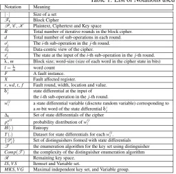
Figure 1: Fault propagation in impossible differential fault attack on AES and formation of the IDFA property (marked in red). None of the variables in this state differential can assume the value 0 for the correct key guess.
Definition 3. [Distinguisher Criteria]A state differentialδijis called a distinguisher if the entropy H(δij)is less than the maximum entropy of the state differential.
The main idea of our dynamic distinguisher identification scheme is to learn the distinguishers from the fault simulation data, acquired from the executable cipher model by varying the plaintexts,
keys, and the fault values. Let us consider the differential execution trace∆kcorresponding to a
faultF. The values assumed by the variables associated with∆kvary with the change of plaintext,
key and the fault value. Such variations result in a fault simulation dataset which is analyzed to identify distinguishers. Let us denote the datasets corresponding to each state differentialδijasTδi
j.
EachTδi
j is a table, containingl,m-bit variablesw i j
z (1≤z≤l) and data values, corresponding to
each of them. For convenience, we further denote each column of aTδi
j asTwi jz. Corresponding to
each fault according to our formalization, we have many such tables corresponding to each state differential in∆k. Typically, a subset of the possible state differentials actually qualifies as potential distinguishers. We denoteT∆k=hTδr1,Tδr2, ....,Tδrd, ...,TδR1,TδR2, ....,TδRdias the set of the tables for
the state differentials. Our data-based framework tests eachδijseparately and decides whether it
constructs a distinguisher. Two distinct cases can be identified in the course of the distinguisher identification which we outline next.
3.1.1 Case 1. The Variables are Independent, but not Uniform within the Complete Range:
In this typical case, the probability distributions of individual state differential variables change, while they still remain independent. Decrease in individual entropies of the variables due to
their non-uniformity over the complete range[0,2m−1](note that uniformity may still hold over
some sub-range of[0,2m−1]), causes a drop in the total state differential entropy. The situation
is described in Algorithm1, where the changed probability distributions are denoted as p0zwi j
(z=1,2, ...,l), and the joint state differential entropy asHInd(δji) =∑lz=1(−∑2
m−1
q=0 p
0wi jq
z log2(p0
wi jq
z )).
Each column of the tableTδi
j (denoted as Twi jz), corresponding to each variablew
i j
z is treated
separately for missing values (if any) within the range of[0,2m−1]. As a concrete example, if a
state differential pose an impossible differential property, none of thewi jzs can assume value 0, and
as a result, the value 0 will be missing in the tableT
wi jz for anyz. Information regarding the values
which are not missing are important in the context of the distinguisher and hence preserved for eachwi jz in the setRngwi j
z. Typical examples of Case. 1 include the IDFA attack on AES and the
attack on PRESENT described in [JLSH13].
Table 2: Frequent Itemset Mining: Toy Example
TID v1 v2 v3 v4 v5
1 1 5 7 8 11
2 2 4 6 9 13
3 1 5 7 10 2
4 2 4 6 11 4
5 3 9 8 6 5
6 1 10 11 9 8
SB
Ciphertext Difference SB
SB
SR SR
SR
MC
MC
f f’ f’ 2f’
f’ f’
3f’
2f1f4 f33f2
f1 f43f32f2
f13f42f3f2
3f12f4f3 f2
f5 f9f13f17
f6f10f14f18
f7f11f15f19
f8f12f16f20
f5 f9f13f17
f10f14f18f6
f15f19f7f11
f20f8f12f16
f1
f2
f3
f4
f1
f2
f3
f4
8 9 10
Figure 2: Fault propagation in AES with the fault injected at the beginning of 8-th round. Distin-guisher is formed at the input of the 10-th round S-Box (marked in red)
used in IDFA attacks to distinguish correct key guesses from wrong ones. For the IDFA attack on AES, a byte fault is injected at the beginning of the 7-th round of the cipher resulting in some state differentials none of whose variables can assume the value 0, with the correct key guess. The
situation is elaborated in Fig.1, where each large square represents an intermediate state differential
of AES, with the fault injected at the beginning of the 7-th round in the 0-th byte location. Each small square in the figure represents a state differential variable of size one byte. The shaded
states in Fig.1denote the existence of an impossible differential, with all bytes being active (fault
difference cannot be 0). It is convenient to use the last among them as a distinguisher due to its
proximity to the ciphertext (marked red in Fig.1).
It is apparent that the distinguisher identification framework of ours identify this impossible
differential property as an instance of case 1. TheRngChkfunction detects the absence of 0 in each
of the variables, and as a result, the entropy becomesHInd(δ93) =∑16z=1(−∑2
8−1
q=0 p
0wi jq
z log2(p0
wi jq
z )) =
∑16z=1(−0−∑ 28−1
q=1 2551 log2(2551 )) =∑ 16
z=1(−255×2551 log2(2551 )) =127.90, which makes the state
differential qualify as a distinguisher. One should note that, the state differentialsδ91andδ92also
possess the impossible differential property and are detected by theRngChkroutine.
Example 2: A Distinguisher on PRESENT In this example, a fault is injected at the beginning of the 28-th round of the PRESENT cipher. The width of the fault is of 16 bits. The distinguisher identification algorithm, in this case, identify the input state of the S-Box of the
30−thround (δ301) as the best distinguisher. TheRngChkfunction identifies that each of the 4 bit
variables in this state differential can assume only 2 values among 24possible values (although
the 2 values assumed may change depending on the fault locations), and as a result, the entropy becomesHInd(δ302) =∑16z=1(−2×12log2(12)) =16.
3.1.2 Case 2. The Variables are not Independent
The second case of the distinguisher identification problem deals with the scenarios where correlations exist between some of the variables within a state differential, which eventually cause the reduction of state differential entropy. Typical examples exist for the ciphers with MDS matrices. Detection of the associations/correlations among the variables is crucial for calculating the entropyHAssn(δij) =H(w
i j
1,w
i j
2, ...,w
i j
l )in this case. We utilize well-known association rule
mining (itemset mining) strategies for this purpose.
Frequent Itemset and Association Rule Mining:
mining, which refers to the discovery of association relationships or correlations among a set
of items. Formally, given a large number of variables (attributes) (var1,var2, ...,varn), and a
table/database of values they assume within their respective domains, anitemis defined asvarq=
val, wherevallies in the domain ofvarq. The simplest case occurs while dealing with
discrete-valued variables having small ranges, where each item can be defined precisely. IfI={i1,i2, ...,ia}
is a set of all items constructed from a table of discrete valued variables, then anyIs⊂Iis called
anitemset. The prime task of an association rule mining algorithm is to figure out associations (if
any) of the formA⇒B, where bothAandBare propositional logic formulae over the items.
In the present context, we are mainly interested in itemsets and the variables associated with
them. The number of all possible itemsets are exponential with the size ofI, and most of them
are not interesting for practical purpose. This fact leads to the finding of itemsets occurring
frequently in a table, which is known asfrequent itemset mining. The frequent itemset mining task
is governed by a statistical parametersupport, which represents the frequency of occurrence of
an itemset in the database. Formally support of an itemsetIsin a table/databaseDBis defined as,
supp(Is) =|Is(ti)|/|DB|, whereIs(ti) ={ti|ti is an entry in DB and ti contains Is}. An itemset is called a frequent itemset if its support is greater than or equal to some predefined minimum
support value. Further, an itemset is called amaximal frequent itemsetif none of its immediate
supersets is frequent.
To illustrate the above-mentioned concepts precisely, let us consider the toy database presented in
Table.2. There are 5 discrete valued variables in this table having value ranges from 1 to 13. We
set the support as 26=0.33. It can be easily figured out from Table.2, that there are two itemsets of size 3, beyond this support threshold – namely(v1=1,v2=5,v3=7)and(v1=2,v2=4,v3=6).
It is worth to note that, no superset of these itemsets are frequent (that is, these are the maximal frequent itemsets), and all subsets of these are frequent. Further, it is interesting to note that, for
variablev4andv5all the itemsets are of cardinality 1. Intuitively, this implies that the variables
v4andv5are statistically uncorrelated. Note that, setting the proper support is imperative, as
otherwise, one may obtain a large number of itemsets of little practical interest.
Finding Itemsets within State Differentials:
In the context of distinguisher identification, we are mainly interested in the maximal frequent itemsets within some reasonable support. The key idea is to figure out the variables within a state
differential, which are strongly correlated. For this purpose, we utilize the well-knownApriori
association rule mining framework. The complete procedure is described in Algorithm2. The
algorithm takes aTδi
j as input, which is then fed to theApriorifunction after some basic
prepro-cessing. From, each of the itemsets generated by the miner, we separate out the variables and create
sets calledVariable Sets. Variables within the same variable set are dependent, whereas they are
assumed to be independent across different variable sets. Multiple itemsets exist corresponding to eachVariable Setand a table is formed which stores eachVariable Set, along with its corresponding itemsets. This table contains complete information regarding the distinguisher of our interest
and is represented here as a pair(V Sδi
j, {IS
v
δij}
|V S
δij|
v=1
), whereV Sδi
j denote the set of all variable
sets and{ISv δij}
|V S
δij|
v=1
denote the set of itemsets corresponding to each variable setv. Next, the
state differential entropy is calculated using this table, which involves the calculation of the joint
distribution followed by the joint entropy of each variable setv∈V Sδi
j (line 6-8 in Algorithm2).
Using the independence assumption of the variable sets, these entropies can be summed up giving the total entropy of the state asHAssn(δij).
Example 3. A Distinguisher for AES with a Byte Fault Injected at the Beginning of
8-th Round: This example elaborates the case 2 of the distinguisher identification problem. In this attack a byte fault is injected at the 0th byte of AES state at the beginning of 8th round. The
is the output of the 9-th round MixColumn. This state differential achieves the smallest entropy value and is eventually selected as the potential distinguisher for the attack. We now elaborate the entropy calculation for this state differential. The state differentialδ101 =hw1101 ,w1102 , ...,w110l i
contains 16 state differential variables, each with bit-widthm=8. The maximum entropy here is
Hmax(δ101) =128. However, the functionMinerreveals variable associations. More specifically,
there are 4 variable sets(w110
1 ,w1102 ,w1103 ,w1104 ),(w1105 ,w1106 ,w1107 ,w1108 ),(w1109 ,w10110,w11011 ,w11012 ),
and(w11013 ,w11014 ,w11015 ,w11016 )(variable numbering was done column-wise maintaining the convention
in AES), each having 255 itemsets for them. The joint entropy of each variable setvbecomes
HAssn(v) =∑255q=12551 log2(255) =7.99, which finally results in the state differential entropy of HAssn(δ101) =4×7.99=31.96.
Complete Distinguisher Identification Flow:
The complete distinguisher identification algorithm takes the datasetT∆k=hTδr1,Tδr2, ....,TδRdias
input, and outputs a setDist={hDi
j,Hiji}, whereDijis a distinguisher corresponding to the state
δij (only ifδij satisfies the distinguishing criterion), andHij is the entropy of this distinguisher.
The entropyHijis typically the minimum ofHInd(δij),HAssn(δji)(returned byRngChkandMiner, respectively), andHmax(δij)(calculated according to the Definition2). Indeed,Hij<Hmax(δij)is the essential criterion for a state differential to qualify as a distinguisher. It is worth to note that,Di j
contains the complete description of a distinguisher, obtained by combining the outputs ofRngChk
andMiner, given by,Dij:=h{wi jz}lz=1, {Rngwi jz} l
z=1,V Sδij,{IS
v
δij}
|V S
δij|
v=1
i. The pseudocode for this
algorithm is rather straightforward and is thus omitted here.
Determining the proper distinguisher:
The distinguisher identification step usually returns a set of potential distinguishers with their respective entropies specifying their qualities. In general, the distinguisher having the lowest entropy is the best for obvious reasons. However, the evaluation complexity of a given distinguisher plays a crucial role in its selection for a practical attack, as will be shown in the next subsection. After the completion of the first phase of the algorithm, we simply retain all the discovered distinguishers. This is because their usefulness is difficult to decide at this point. However, some of the distinguishers can be instantly eliminated based on some simple rules. It is mandatory to have an S-Box between any distinguisher and the ciphertext. In an even strict sense, if one intends to extract round keys from a specific round with a given distinguisher, he/she must have an S-Box between the distinguisher and the key addition step. Otherwise, the difference equations for key extraction cannot be constructed. Based on this rule, one can clearly eliminate some of the distinguishers, if possible. A concrete example of such a situation is discussed in the next section in the context of IDFA attack on AES.
3.2
Enabling Divide-and-Conquer in Distinguisher Enumeration
algo-rithm
T
Injection of a fault results in a set of distinguishers with different entropy values, as shown in the previous subsection. However, only a few of them are practically utilizable for attack, as the usability of a distinguisher depends on the complexity of evaluating it exhaustively. In DFA, the distinguishers are evaluated in the form of a system of difference equations (or inequations) and the solution space of the system results in a reduced set of candidate keys containing the correct key. Given this system, the practicality of a DFA attack depends on two factors:
1. Distinguisher Evaluation Complexity: The complexity of exhaustively enumerating the system for all possible key guesses.
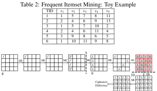
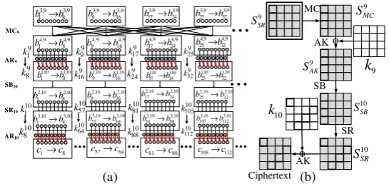
1,30 1 b 1,30 2 b 1,30 3 b 1,30 4 b 2,30 1 b 2,30 3 b 2,30 4 b 2,30 2 b 3,31 1 b 1 c 32 1 k 30 1 k 3,31 5 b 3,31 9 b 3,31 13 b 32 5 k 32 9 k 32 13 k 5 c 9 c 13 c (a) (b) . . . . . . . . 2,9 2,9 1 8 b→b b92,9→b2,916
2,9 2,9 17 24 b→b
3,9 3,9 1 8
b→b b93,9→b163,9 b3,917→b3,924 2,9 2,9 25 32 b→b
3,9 3,9 25 32 b→b (c)
(d)
Figure 3: Example: Subgraphs corresponding to different sub-operations of a cipher
Following the notation described in Eq.5, we denote theDistinguisher Evaluation Complexity
withComp(T)whereT is the distinguisher enumeration algorithm andComp(·)denotes the
complexity of an algorithm. TheOffline Complexity, on the other hand, is denoted with|R|where
Ris the remaining key space after distinguisher evaluation. TheComp(T)and the|R|, can be
estimated once the systems of equations for the distinguishers are in place. TheAttack Complexity
of a DFA can be determined as:
Comp(A) =max(Comp(T),|R|) (6)
One should note that, the definition of attack complexity at this point assumes that only one fault instance has been injected. The attack complexity indeed depends on the number of faults injected. However, for most of the cases the required number of injections for making an attack practical
can be determined from the value ofComp(A)with a single fault instance and so we define it in
terms of a single injection.
Knowing the systems of difference equations apriori, is not a very practical assumption for an automated tool, as it depends upon the distinguisher(s) chosen. The most critical factor associated with distinguisher evaluation is to choose a proper divide-and-conquer strategy for enumerating the solution space of the difference equation system. Instead of guessing the complete key at once (which has a prohibitively large complexity), such a strategy allows guessing small key parts exhaustively and as a result the correct key can be recovered in parts with a practical time complexity. In this work, we construct such equation systems automatically in an abstract form, which is suitable for the purpose of attack complexity evaluation. Further, this abstract description can be extended to concrete fault difference equations, if required. To automatically determine
the divide-and-conquer strategy we propose a graph based abstraction of the cipher calledCipher
Dependency Graph(CDG). Let us represent each statesijassij=hbi j1,bi j2, ....,bi j
λi, where eachb
i j z
corresponds to abit variable1. Given this representation of the states, we define the CDG for a
block cipher as follows:
Definition 4. [Cipher Dependency Graph]A Cipher Dependency Graph (CDG) for a block cipher is a directed acyclic graph (DAG)GhV,Ei, where every node v∈Vcorresponds to a bit
variable bi jz (1≤z≤λ) at the input of round j and sub-operation i of the cipher. A directed edge e∈Erepresents the dependency between two bit variables belonging to two consecutive states sij
and sij+1(or s1j+1) imposed by the sub-operation oij+1at the abstraction level of bits, considering
the bit variable of sijas input, and that of sij+1as the output, respectively.
Certain simplifying assumptions were made, while constructing the CDGs. Some basic CDG
building blocks are illustrated in Fig.3. For the S-Boxes, we assume that each output variable is
dependent on all the S-Box inputs (Fig.3(a)). The key addition operations are represented by
structures shown in Fig.3(b). Permutation layers are often straightforward and thus not shown here.
AR31 1,30 1 b 3,31 1 b 1 c 32 1 k
...
...
...
... ... ... ... ... ... ... ... ... ... ... ... ... ... ......
...
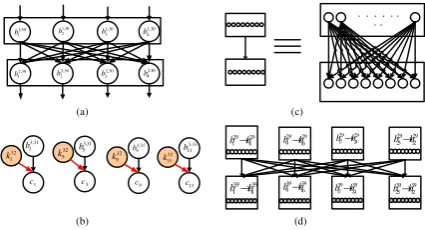
... SB30 P30 SB31 P31 AR32 1,30 2 b 1,30 3 b 1,30 4 b 1,30 5 b 1,30 6 b 1,30 7 b 1,30 8 b 1,30 9 b 1,30 10 b 1,30 11 b 1,30 12 b 1,30 13 b 1,30 14 b 1,30 15 b 1,30 16 b 2,30 1 b 2,30 2 b 2,30 3 b 2,30 4 b 2,30 5 b 2,30 6 b 2,30 7 b 2,30 8 b 2,30 9 b 2,30 10 b 2,30 11 b 2,30 12 b 2,30 13 b 2,30 14 b 2,30 15 b 2,30 16 b 3,30 1 b 3,30 2 b 3,30 3 b 3,30 4 b 31 1 k 31 2 k 31 3 k 31 4 k 1,31 1 b 1,31 2 b 1,31 3 b 1,31 4 b 2,31 1 b 2,31 2 b 2,31 3 b 2,31 4 b 3,30 1 b 3,30 2 b 3,30 3 b 3,30 4 b 31 17 k 31 18 k 31 19 k 31 20 k 1,31 17 b 1,31 18 b 1,31 19 b 1,31 20 b 2,31 17 b 2,31 18 b 2,31 19 b 2,31 20 b 3,30 1 b 3,30 2 b 3,30 3 b 3,30 4 b 31 33 k 31 34 k 31 35 k 31 36 k 1,31 33 b 1,31 34 b 1,31 35 b 1,31 36 b 2,31 33 b 2,31 34 b 2,31 35 b 2,31 36 b 3,30 49 b 3,30 50 b 3,30 51 b 3,30 52 b 31 49 k 31 50 k 31 51 k 31 52 k 1,31 49 b 1,31 50 b 1,31 51 b 1,31 52 b 2,31 49 b 2,31 50 b 2,31 51 b 2,31 52 b 32 5 k 3,31 5 b 5 c 32 9 k 3,31 9 b 9 c 32 13 k 3,31 13 b 13 c 32 17 k 3,31 17 b 17 c 32 21 k 3,31 21 b 21 c 32 25 k 3,31 25 b 25 c 32 29 k 3,31 29 b 29 c 32 33 k 3,31 33 b 33 c 32 37 k 3,31 37 b 37 c 32 41 k 3,31 41 b 41 c 32 45 k 3,31 45 b 45 c 32 49 k 3,31 49 b 49 c 32 53 k 3,31 53 b 53 c 32 57 k 3,31 57 b 57 c 32 61 k 3,31 61 b 61 cFigure 4: Example: Finding Key Parts for the Distinguisher Evaluations in PRESENT
However, some linear operations like MDS matrices need special care (more specifically the linear
layers which involves XOR operations). Fig.3(d) represents one such scenario for 8-bit variables,
which are shown in groups for convenience. The MDS structures are also complete graphs (of 32
vertices in this example). It is worth to mention that, the graphG is completely cipher-specific, and
thus one needs to construct it only once while doing the exploitable fault analysis for a specific
cipher. A CDG, corresponding to a fault attack test case on PRESENT is illustrated in Fig.4. For
ease of understanding, only the sub-graph relevant to an attack example is shown1. Interestingly,
the CDG is already divided into clearly identifiable levels.
Construction of a Divide and Conquer Strategy:
The next step to the CDG construction is the identification of independent key parts to be guessed. For a given distinguisher, we initiate a series of breadth first searches (BFS) up to the ciphertexts nodes of the CDG. Each BFS search begins with a bit variable at the state, where the distinguisher has been constructed. The search typically figures out all the mutually dependent bit variables
starting from the start node, in the form of the BFS tree (refer to Fig.4for example). Once the
BFS tree is obtained, one can figure out the key nodes attached to it inO(1)complexity.
Example 4: For the sake of illustration, let us refer to Fig.4once again. The distinguisher under consideration is the one described in Example 2, which is being constructed at the input
of the 30th round S-Box operation (the first layer of nodes shown in Fig.4.) In the figure, the
colored circles represent the associated state bits one must compute to calculate the first bit in the distinguisher. The key bits one need to guess to calculate the shaded state bits are shown in red, while the associated state bits are represented in grey. All the colored variables here are the part of
a BFS tree. Further, from the BFS tree of Fig.4, the key variables to be guessed can be extracted
which are 20 in number for the first bit. In summary, to calculate the first bit of the distinguisher, it is sufficient to guess these 20 bits together and no other key bit is required to be guessed. This provides the divide-and-conquer we require.
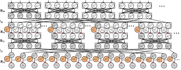
Optimizations: Certain intricacies are there to be taken care of while collecting the independent key parts for a distinguisher. Interestingly, not all key variables obtained by the BFS search are
necessary. To illustrate this, we refer to the Fig.5(a), which corresponds to the partial CDG for the
IDFA attack on AES.2For convenience, the word level representation of the CDG is also provided
along with (Fig.5(b)). It is easy to observe from the word level representation that the key bits
corresponding tok9are not required to be guessed for distinguisher evaluation. The reason behind
this fact is that there is no nonlinear layer between the key variables ink9and the distinguisher
inS9SR. As a result, these key variables get cancelled out with the calculation of the differential.
However, these key variables will still be detected by the BFS based search. Fortunately, we can
3,9 3,9
1 8
b →b b93,9→b163,9
3,9 3,9
17 24
b →b
MC9
4,9 4,9
9 16
b →b 4,9 4,9
17 24
b →b
4,9 4,9
1 8
b →b
3,9 3,9
25 32
b →b
4,9 4,9
25 32
b →b
AR9
1,10 1,10
1 8
b →b 1,10 1,10
9 16
b →b 1,10 1,10
17 24
b →b b1,1025→b1,1032
SB10
SR10
3,10 3,10
1 8
b →b
1 8
c →c
AR10
3,10 3,10 57 64
b →b
57 64
c →c
3,10 3,10 81 88
b →b
81 88
c →c
3,10 3,10 105 112
b →b
105 112
c →c
...
...
...
...
...
...
2,10 2,10
1 8
b →b b92,10→b162,10 b172,10→b242,10
2,10 2,10 25 32
b →b
SB SR MC AK AK 9 SR S 9 MC S 9 AK S 10 SB S 10 SR S Ciphertext 9
k
10 k (a) (b) 9 1 k 9 8 k 9 9 k 9 16 k 9 17 k 9 24 k 9 25 k 9 32 k 10 1 k 10 8 k 10 57 k 10 64 k 10 81 k 10 88 k 10 105 k 10 112 kFigure 5: Example: Finding Key Parts for the Distinguisher Evaluations in AES:
easily enhance the proposed mechanism to encompass such scenarios. The idea is to keep the track of the non-linear layers (S-Boxes) encountered, at each level of the CDG during the BFS traversal. This can be easily done by maintaining counters within the nodes of the CDG. While collecting the key variables, if it is found that the level corresponding to the key variables is not preceded by any
S-Box level, the keys can be discarded. Referring to Fig.5(a), the key nodes in blue color thus can
be discarded. The first bit of this distinguisher can be evaluated by guessing just 32 key bits ofk10.
Calculation of the Distinguisher Evaluation Complexity: The BFS based key part finding algorithm actually returns sets of key bits, corresponding to each bit of the distinguisher state.
However, in order to calculate the quantitiesComp(T)and|R|we need to exploit some more
structural properties of the cipher, already present in the CDG. As for most of the time, we are
dealing withmbit distinguisher variables, it is trivial to combine the key bit sets corresponding
to eachmbit variable. One should also consider combining the key bit sets corresponding to the
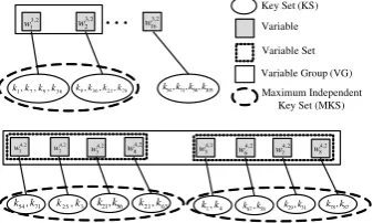
variable sets (if any). While evaluating any of these variables/variable sets, the corresponding keys must be guessed simultaneously. At this point, certain other things are to be taken care of. Let us consider a distinguisherδij=hwi j1,wi j2, ...,wi jli. Corresponding to eachwi jz, there exists a set of key bit variables. An obvious way is to view the relationships as a bipartite graph, as
shown in Fig6. Without loss of generality, we just consider variables and not the variable sets
in this discussion, although the same logic applies to the later one. Let us denote the key set
corresponding to each variablewi jz asKey Set(KSz). The key sets, however, may have overlaps.
As a concrete example, one may consider the PRESENT case study depicted in Fig.4. All 4
consecutive nibbles in the distinguisher at round 30 (shown in the diagram as layerSB30), depends
upon the same 16 round key bits from the last round. Such overlaps are extremely important from the divide-and-conquer point of view. This is because, the overlaps indicate that all the difference
equations, that can be constructed involving these key bits and the associated variableswi jz will
share the key variables. As a result they must be evaluated simultaneously. Putting it in a more simplified manner, if there are overlaps, computation related to all the overlapping variables must
be performed simultaneously. To deal with such cases, we defineMaximum Independent Key Sets
(MKS), which are non-overlapping subsets of key variables, constructed by taking the union of
overlappingKSzs. EachMKShalso impose a grouping on the correspondingwi jzs attached to its
component KSs. We call such groupings asVariable Groups(VG).1Intuitively, eachhV Gh,MKShi
tuple refers to a set of independent equations to be solved for the key extraction. In our graph based
representation, we informally refer them asindependently computable chunks/subparts.
Calculation ofComp(T)becomes trivial after the above-mentioned grouping. Let us consider,
an MKS asMKShand the corresponding variable group asV Gh(note that variable groups may
also include variable sets as its elements.). EachV Ghcan be evaluated independently. Let us
1Note that we have used the term “group” to differentiate it from the variable sets. From this point onwards, we shall
. . .
1,7,9,36
k k k k k9,k36,k21,k78 k54,k71,k58,k105
54,71
k k
2 5,3
k k k21,k56 k21,k63 k1,k4 k67,k58 k29,k31 k78,k87 3,2
1
w 3,2
2
w 3,2
16
w
4,2 1
w 4,2
2
w 4,2
3
w 4,2
4
w 4,2
5
w 4,2
6
w 4,2
7
w 4,2
8
w
Key Set (KS)
Variable
Variable Set
Variable Group (VG)
Maximum Independent Key Set (MKS)
Figure 6: Illustration of the Relationships between Key and Distinguisher Variables
assume that we haveMsuchV Ghs along with their correspondingMKShs. The time complexity of
computing each of them is given asComp(Th) =2|MKSh|, 1≤h≤M. It is quite obvious that such
a search can be performed (and should be) in a parallel manner. As a result, the overall complexity
of the distinguisher enumeration algorithmT becomes:
Comp(T) =maxh(Comp(T1),Comp(T2), ...,Comp(TM)) (7)
Example 7. IDFA attack on AES: In this example, we figure out the evaluation complexity of the IDFA diatinguisher. It is observed that each byte of the distinguisher depends on 32 key bits from the 10-th round. Further, 4 consecutive state differential variables are found to depend on
the same 32 key bits. Following our notation size of eachV Ghhere is 4 state differential variables
and the associatedMKShcontains 32 bits of key. Clearly, the distinguisher evaluation complexity
Comp(T)becomes 232in this case.
Example 8. AES with 8th round fault injection: In this case, the distinguisher consists of 4 variable sets, containing 4 variables each. Each 8-bit variable in the distinguisher state depends on 8 consecutive key bits (that is key bytes), and with the existence of variable sets having cardinality
4, one must consider 8×4=32 key bits simultaneously, for guessing (i.e.|MKSh|=32). Further,
the key bytes associated with each variable set are independent, and hence eachV Ghwill contain
only a single variable set. Overall,Comp(T) =232.
Example 9. PRESENT with 28th round fault injection: The distinguisher here is formed
at the input of the 30-th round S-Box. As it can be seen from Fig.4, each distinguisher bit (actually
each nibble) here depends on 20 key bits. However, due to the overlappings present in different nibble-wise key sets (KSs), the distinguisher evaluation process can eventually be partitioned into 4
independent(MKS,V G)pairs, each having 32 key bits involved – 16 from the last round and rest
from the penultimate round. The size of correspondingV Ghs become 4 state differential variables
each. As a result,Comp(T)becomes 232.
3.3
Complexity Evaluation of the Remaining Key Space
R
The final step in finding a successful DFA is the evaluation of the remaining keyspace size (|R|)
after the fault injection. Often, the complexity remains beyond the practical exhaustive search complexity with a single fault injection and as a result, one might require multiple faulty ciphertexts. Nevertheless, the required number of faults for the successful attack can be estimated from the remaining space complexity of a single injection, and hence we specifically focus on the remaining
search space with a single fault. A distinguisherDij and the corresponding key parts obtained
in the last two steps can be utilized to figure out the remaining keyspace complexity efficiently.
Another important component of this computation is thedifferential characteristicof the S-Boxes.
S-Box differential equation may have. They can be calculated from the Differential Distribution
Tables (DDT) of S-Boxs. The DC values for different ciphers can be found in [KRH17].
The algorithm for remaining search space evaluation is presented in Algorithm3. The main
idea in this step is to figure out the probability, with which the distinguishing property occurs during distinguisher enumeration with random key guesses. This probability is then multiplied with the total key space in the corresponding MKS, giving the remaining search space complexity.
Referring to the algorithm, the input consists of the corresponding distinguisherDi
j, and a set of
tuples with cardinalityM, which contains the MKSs and corresponding VGs. As an additional
component, the DC characteristic of the S-BoxesHShcorresponding to eachMKSh, V Ghpair
is also supplied. TheHShis the DC value corresponding to each(MKSh, V Gh)pair. In some
cases, a distinguisher may involve multiple S-Box layers and as a resultHShshould be multiplied
many times for each distinguisher variable (or variable set) evaluation. To keep things simple we
directly provide the algorithm with properly tailored values withinHSh. Values of theHShwith
above-mentioned tailoring can be trivially obtained from the CDGs described in the last subsection, just by keeping track of the S-Boxes encountered with the distinguisher.
Example 9. IDFA attack on AES: In this case, it turns out that|R|V G1 =2
32×(255 28 )4
(roughly equal to 232−226). This is because each state differential variable inV G1assumes the
distinguishing property with probability 255
28 and there are 4 such variables inV G1. The size of
the remaining keyspaces are the same for other threehMKSh,V Ghipairs. The large size of the
remaining keyspace indicates the need of multiple fault injection. Although, the estimation of the required number of faults here is slightly nontrivial due to the impossible differential inequalities
involved, it can be estimated using the construction from [DFL11]. Overall, the attack complexity
isO(232)and total 211faults will be required to extract the key uniquely [DFL11].
Example 10. AES with 8th round fault injection: The MKS and VGs, which are the inputs
to the Algorithm3are 4 in number in this case. Further, each VG contains a single variable set and
32 key bits corresponding to that. One needs to consider the number of itemsets corresponding to each variable set (or variable group, as in this case each group contains a single variable set) in this case. For each of the 4 variable sets, the probability of occurrence of the distinguishing criterion
isP[V Gh] = 255232. The DC characteristic of AES S-Box is found to be 1 and the total number of
key possibilities are 232. The remaining keyspace corresponding to each variable set thus becomes
232×2−24=28, leading to a complete remaining search space complexity of(28)4=232. One
should exhaustively search this remaining keyspace for the correct key. The total complexity of the
attack, considering bothComp(T)and|R|thus remains 232.
In [TMA11], Tunstall et. al. presented a 2 step approach for the attack described here, which
eventually reduces the remaining keyspace size to 28. The idea is to complete the attack just
described, and then to exploit another distinguisherδ91which was previously costly to evaluate
on the complete keyspace. However, one should notice that the attack complexity still remains
232. The distinguisher identification framework of ExpFault detects both the distinguishers. The
two-step attack requires the existence of the inverted key schedule equations. The proposed tool in its current form requires some manual intervention to handle attacks using multiple distinguishers. In future versions of the tool this dependency will be removed. However, it is worth mentioning that, the results already outputted by the tool are sufficient to easily discover such attacks.
Example 11. Attack on PRESENT: The distinguisher evaluation process, in this case, can
eventually be partitioned into 4 independenthMKSh,V Ghipairs, each having evaluation complexity
of 232. For each of the 4(MKSh,V Gh)pair, the probability of occurrence of the distinguishing
criterion isP[V Gh] = (162)4=2−12, and the remaining key space size is|R|V Gh =2
20. With a
single fault injection, thus the keyspace reduces to 280from 21281in this case, and the attack
1The distinguisher here simultaneously extracts round keys from last two rounds of PRESENT. Total 128 key bits are