An Improved RNS Variant of the BFV
Homomorphic Encryption Scheme
Shai Halevi?1, Yuriy Polyakov??2, and Victor Shoup3
1
IBM Research
2 NJIT Cybersecurity Research Center
3 NYU
December 5, 2018
Abstract. We present an optimized implementation of the Fan-Vercauteren variant of Brakerski’s scale-invariant homomorphic encryption scheme. Our algorithmic improvements focus on optimizing decryption and ho-momorphic multiplication in the Residue Number System (RNS), using the Chinese Remainder Theorem (CRT) to represent and manipulate the large coefficients in the ciphertext polynomials. In particular, we propose efficient procedures for scaling and CRT basis extension that do not require translating the numbers to standard (positional) rep-resentation. Compared to the previously proposed RNS design due to Bajard et al. [3], our procedures are simpler and faster, and introduce a lower amount of noise. We implement our optimizations in the PAL-ISADE library and evaluate the runtime performance for the range of multiplicative depths from 1 to 100. For example, homomorphic multi-plication for a depth-20 setting can be executed in 62 ms on a modern server system, which is already practical for some outsourced-computing applications. Our algorithmic improvements can also be applied to other scale-invariant homomorphic encryption schemes, such as YASHE.
Keywords: Lattice-Based Cryptography · Homomorphic Encryption · Scale-Invariant Scheme·Residue Number Systems·Software Implementation
1
Introduction
Homomorphic encryption has been an area of active research since the first design of a Fully Homomorphic Encryption (FHE) scheme by Gentry [9]. FHE allows performing arbitrary secure computations over encrypted sensitive data without ever decrypting them. One of the potential applications is to outsource computations to a public cloud without compromising data privacy.
?Supported by the Defense Advanced Research Projects Agency (DARPA) and Army
Research Office (ARO) under Contract No. W911NF-15-C-0236.
?? Supported by the Sloan Foundation and Defense Advanced Research Projects
A salient property of contemporary FHE schemes is that ciphertexts are “noisy”, where the noise increases with every homomorphic operation, and de-cryption starts failing once the noise becomes too large. This is addressed by setting the parameters large enough to accommodate some level of noise, and using Gentry’s “bootstrapping” technique to reduce the noise once it gets too close to the decryption-error level. However, the large parameters make homo-morphic computations quite slow, and so significant effort was devoted to con-structing more efficient schemes. Two of the the most promising schemes in terms of practical performance have been the BGV scheme of Brakerski, Gentry and Vaikuntanathan [6], and the Fan-Vercauteren variant of Brakerski’s scale-invariant scheme [5,8], which we call here the BFV scheme. Both of these schemes rely on the hardness of the Ring Learning With Errors (RLWE) problem.
Both schemes manipulate elements in large cyclotomic rings, modulo integers with many hundreds of bits. Implementing the necessary multi-precision modular arithmetic is expensive, and one way of making it faster is to use a “Residue Number System” (RNS) to represent the big integers. Namely, the big modulusq
is chosen as a smooth integer, q = Q
iqi, where the factors qi are same-size, pairwise coprime, single-precision integers (typically of size 30-60 bits). Using the Chinese Remainder Theorem (CRT), an integer x∈Zq can be represented by its CRT components{xi=xmodqi ∈Zqi}i, and operations on xin Zq can be implemented by applying the same operations to each CRT componentxiin its own ringZqi.
Unfortunately, both BGV and BFV feature some scaling operations that can-not be directly implemented on the CRT components. In both schemes there is sometimes a need to interpret x∈Zq as a rational number (say in the interval [−q/2, q/2)) and then either lift xto a larger ring ZQ for Q > q, or to scale it down and round to get y = dδxc ∈ Zt (for some δ 1 and accordingly
tq). These operations seem to require thatxbe translated from its CRT rep-resentation back to standard “positional” reprep-resentation, but computing these translations back and forth will negate the gains from using RNS to begin with. While implementations of the BGV scheme using CRT representation are known (e.g., [10, 12]), implementing BFV in this manner seems harder. One dif-ference is that BFV features more of these scaling operations than BGV. Another is that in BGV numbers are typically scaled by just single-precision factors, while in BFV these factors are often big, of order similar to the multi-precision mod-ulus q. An implementation of the BFV scheme using CRT representation was recently reported by Bajard et al. [3], featuring significant speedup as compared to earlier implementations such as in [15]. This implementation, however, uses somewhat complex procedures, and moreover these procedures incur an increase in the ciphertext noise.
We implemented our procedures in the PALISADE library [18]. We evaluate the runtime performance of decryption and homomorphic multiplication in the range of multiplicative depths from 1 to 100. For example, the runtimes for depth-20 decryption and homomorphic multiplication are 3.1 and 62 ms, respectively, which can already support outsourced-computing applications with latencies up to few seconds, even without bootstrapping.
1.1 Our contributions
We propose new techniques for CRT basis extension and scaling in RNS using floating-point arithmetic for some intermediate computations. Our CRT basis extension and scaling procedures have a low probability of introducing small ap-proximation errors, but in the context of homomorphic operations these errors are inconsequential. As we explain in Section 4.5, they increase the ciphertext noise after homomorphic multiplications by at most 2 bits for any depth of the multiplication circuit (typically significantly less than 1 bit), and those contri-butions were not observable in our experiments. We apply these techniques to develop:
– A BFV decryption procedure in RNS that supports CRT moduli up to 59 bits, using extended precision floating-point arithmetic natively available in x86 architectures.4
– A BFV homomorphic multiplication procedure that has practically the same noise requirements as the textbook BFV.
– A multi-threaded CPU implementation of our BFV RNS variant in PAL-ISADE.
We show that our procedures are not only simpler, but also have lower com-putational complexity and noise growth than the procedures presented in [3].
2
Notations and Basic Procedures
For an integer n ≥ 2, we identify below the ring Zn with its representation in the symmetric interval Z∩[−n/2, n/2). For an arbitrary real number x, we denote by [x]n the reduction of x into that interval (namely the real number
x0 ∈[−n/2, n/2) such that x0−xis an integer divisible by n). We also denote by bxc, dxe, and dxc the rounding of x to an integer down, up, and to the nearest integer, respectively. We denote vectors by boldface letters, and extend the notations bxc, dxe,dxcto vectors element-wise.
Throughout this paper we fix a set ofkco-prime moduliq1, . . . , qk(all integers larger than 1), and let their product be q = Qk
i=1qi. For all i ∈ {1, ..., k}, we also denote
qi∗=q/qi∈Z and ˜qi=q∗i
−1
(mod qi)∈Zqi, (1)
4
namely, ˜qi∈ −qi 2, qi 2
andqi∗·q˜i= 1 (mod qi).
Complexity measures.In our setting we always assume that the moduliqiare single-precision integers (i.e. |qi|<263), and that operations modulo qi are in-expensive. We assign unit cost to mod-qi multiplication and ignore additions, and analyze the complexity of our routines just by counting the number of mul-tiplications. Our procedures also include floating-point operations, and here too we assign unit cost to floating-point multiplications and divisions (typically in “double float” format as per IEEE 754) and ignore additions.
2.1 CRT Representation
We denote the CRT representation of an integerx∈Zq relative to the CRT basis
{q1, . . . , qk}byx∼(x1, . . . , xk) withxi= [x]qi∈Zqi. The formula expressingx in terms of the xi’s is x=P
k
i=1xi·q˜i·qi∗ (modq). This formula can be used in more than one way to “reconstruct” the value x∈Zq from thexi’s. In this work we use in particular the following two facts:
x=
k
X
i=1
[xi·q˜i]qi·q
∗
i
| {z }
∈Zq
−υ·qfor someυ∈Z, (2)
and x= k
X
i=1
xi·q˜i·qi∗
| {z }
∈[−qiq4 ,qiq4 )
−υ0·qfor someυ0∈Z. (3)
2.2 CRT Basis Extension
Let x∈Zq be given in CRT representation (x1, . . . , xk), and suppose we want to extend the CRT basis by computing [x]p∈Zp for some other modulusp >1.
Using Eq. 2, we would like to compute [x]p =
h Pk
i=1[xi·q˜i]qi·qi∗
−υ·qi
p
.
The main challenge here is to computeυ(which is an integer inZk). The formula forυ is:
υ=
& k
X
i=1
[xi·q˜i]qi·q
∗ i /q % = & k X i=1
[xi·q˜i]qi·
q∗i q % = & k X i=1
[xi·q˜i]qi
qi
%
.
To getυ, we compute for everyi∈ {1, . . . , k} the elementyi:= [xi·q˜i]qi (using single-precision integer arithmetic), and next the rational number zi := yi/qi (in floating-point). Then we sum up all thezi’s and round them to getυ. Once we have the value of υ, as well as all the yi’s, we can directly compute Eq. 2 modulopto get [x]p=
h Pk
i=1yi·[q∗i]p
−υ·[q]p
i
p.
Complexity analysis.The computation ofυrequiresksingle-precision integer multiplications to compute theyi’s, thenkfloating-point division operations to compute thezi’s, and then some additions and one rounding operation. In total it takeskinteger andk+1 floating-point operations. Whenpis a single-precision integer, the last inner product takesk+ 1 integer multiplications, so the entire procedure takes 2k+ 1 integer andk+ 1 floating-point operations.
For larger pwe may need to do k+ 1 multi-precision multiplications, but we may be able to use CRT representation again. Whenp=Qk0
j=1pj for single-precision co-primepj’s, we can computeυ only once and then compute the last inner product for eachpi (provided that we pre-computed [q∗i]pj’s and [q]pj for all i and j). The overall complexity in this case will be kk0 +k+k0 integer operations andk+ 1 floating-point operations.
Correctness. The only source of errors in this procedure is the floating-point operations when computingυ: Instead of the exact valueszi =yi/qi, we compute their floating-point approximations zi∗ (with error i), and so we obtain υ∗ =
dP
i(zi+i)cwhich may be different fromυ=d
P
izic.
Since thezi’s are all in [−12,12), then using IEEE 754 double floats we have that thei’s are bounded in magnitude by 2−53, and therefore the overall magni-tude of the error term:=P
i is bounded,||< k·2−53. If we assumek≤32, this gives us||<2−48. (Similarly, if we use single floats we get||<2−19.)
When applying the procedure above, we should generally check that the resultingυ∗ that we get is outside the possible-error regionZ+12±. Ifυ
∗ falls
in the error region, we can re-run this procedure using higher precision (and hence smaller) until the result is outside the error region.
It turns out that for our use cases, we do not need to check for these error conditions, and can often get by with a rather low precision for this computation. One reason for this is that for our uses, even if we do incur a floating-point approximation error, it only results in a small contribution to ciphertext noise, which has no practical significance.
Moreover, we almost never see these approximation errors, because the value
P
izi that we want to approximate equals x/q modulo 1. When we use that procedure in our implementation, we sometimes have (pseudo)random values of
x ∈ Zq, in which case the probability that the result falls in the error region is bounded by 2||. In other cases, we even have a guarantee that |x| q(say
|x|< q/4), so we know a-priori that the value will always fall outside of the error region. For more details, see Sections 2.4 and 4.5.
2.3 Simple scaling in CRT representation
Let x ∈ Zq be given in CRT representation (x1, . . . , xk), and let t ∈ Z be an integer modulus t ≥2. We want to “scale down” xby a t/qfactor, namely to compute the integery=dt/q·xc ∈Zt. We do it using Eq. 3, as follows:
y:=
t q ·x
=
& k
X
i=1
xi·q˜i·q∗i ·
t q
−υ0·q· t
q
%
=
& k X
i=1
xi·(˜qi·
t qi
) %
−υ0·t =
"& k X
i=1
xi·(˜qi·
t qi
) %#
t
.(4)
The last equation follows since the two sides are congruent modulo t and are both in the interval [−t/2, t/2), hence they must be equal.
In our context,t and theqi’s are parameters that we can pre-process (while the xi’s are computed on-line). We pre-compute the rational numbers tq˜i/qi ∈ [−t/2, t/2), separated into their integer and fractional parts:
tq˜i/qi = ωi+θi, withωi∈Ztandθi∈[−12,12).
With theωi’s andθi pre-computed, we take as input thexi’s, compute the two sumsw := [P
ixiωi]t andv :=dPixiθic, (using integer arithmetic for w and floating-point arithmetic forv), then output [w+v]t.
Complexity analysis.The procedure above takesk floating-point multiplica-tions, some addimultiplica-tions, and one rounding to computev, and then an inner product modtbetween two (k+ 1)-vectors: the single-precision vector (x1, . . . , xk,1) and the mod-tvector (ω1, . . . , ωk, v). When the modulus tis a single-precision inte-ger, theωi’s are also single-precision integers, and hence the inner product takes
k integer multiplications. The total complexity is thereforek+ 1 floating-point operations andkinteger modular multiplications.
For a largertwe may need to doO(k) multi-precision operations to compute the inner product. But in some cases we can also use CRT representation here: Fort =Qk0
j=1tj (with thetj’s co-prime), we can represent eachωi ∈Zt in the CRT basisωi,j = [ωi]tj. We can then compute the resultyin the same CRT basis,
yj = [y]tj by settingwj= [
P
ixiωi,j]tj for allj, and thenyj = [v+wj]tj. This will still take onlyk+ 1 floating-point operations, butkk0 modular multiplications.
Correctness. The only source of errors in this routine is the computation of
v :=dP
ixiθic: Since we only keep the θi’s with limited precision, we need to worry about the error exceeding the precision. Let ˜θibe the floating-point values that we keep, whileθi are the exact values (θi=tq˜i/q−ωi) andiare the errors,
i= ˜θi−θi. Since|θ˜i| ≤ 12, then for IEEE 754 double floats we have|i|<2−53. The value that our procedure computes forv is therefore ˜v :=dP
ixi(θi+i)c, which may be different fromv:=dP
ixiθic.
We can easily control the magnitude of the error term Px
example, if k <32, as long as all our moduli satisfy qi ≤247 <254/4k, we are ensured that|Px
ii|<1/4.
If we use the extended double floating-point precision (“long double” in C/C++) natively supported by x86 architectures, which stores 64 bits in the significand as compared to 52 bits in the IEEE 754 double float, we can increase the upper bound for the moduli up toqi≤259.
When using the scaling procedure for decryption, we can keepy0=dt/q·xc
close to an integer by controlling the ciphertext noise. For example, we can ensure that y0 (and therefore alsov) is within 1/4 of an integer, and thus if we also restrict the size of theqi’s as above, then we always get the correct result. Using the scaling procedure in other settings may require more care, see the next section for a discussion.
2.4 Complex scaling in CRT representation
The scaling procedure above was made simpler by the fact that we scale by at/q
factor, where the original integer is inZq and the result is computed modulot. During homomorphic multiplication, however, we have a more complicated set-ting: Over there we have three parameters t, p, q, where q=Qk
i=1qi as before, we similarly havep=Qk0
j=1pj, and we know thatpis co-prime withqandpt. The input isx ∈ Z∩[−qp/2t, qp/2t) ⊂Zqp, represented in the CRT basis
{q1, . . . , qk, p1, . . . , pk0}. We need to scale it by at/q factor and round, and we want the result modulo q in the CRT basis {q1, . . . , qk}. Namely, we want to computey:=
dt/q·xc
q. This complex scaling is accomplished in two steps: 5 1. First we essentially apply the CRT scaling procedure from Section 2.3 using
q0=qpandt0 =tp, computingy0 := [dtp/qp·xc]p(which we can think of as computingy0 modulo tpand then discarding the mod-t CRT component). Note that since x∈ [−qp/2t, qp/2t) then dtp/qp·xc ∈ [−p/2, p/2). Hence even though we computedy0 modulop, we know thaty0=dt/q·xcwithout modular reduction.
2. Having a representation of y0 relative to CRT basis {p1, . . . , pk0}, we ex-tend this basis using the procedure from Section 2.2, adding [y0]
qi for all theqi’s. Then we just discard the mod-pj CRT components, thus getting a representation ofy= [y0]q.
The second step is a straightforward application of the procedure from Sec-tion 2.2, but the first step needs some explanaSec-tion. The input consists of the CRT componentsxi= [x]qiandx
0
j = [x]pj, and we denoteQ:=qp,Q
∗
i :=Q/qi=q∗ip,
Q0j∗ :=Q/pj =qp∗j, and also ˜Qi = [(Q∗i)−1]qi and ˜Q0j = [(Q0j
∗
)−1]
pj. Then by Eq. 3 we have
t q·x=
t q
k
X
i=1
xiQ˜iQ∗i+ k0
X
j=1
x0jQ˜0
jQ
0
j
∗
−υ0Q
= k
X
i=1
xi·
tQ˜ip
qi +
k0
X
j=1
x0j·tQ˜0
jp
∗
j−tυ
0p.
5
A somewhat different complex scaling procedure with similar complexity is presented in Appendix A.1, which can handle arbitraryx∈Zqp. However we did not implement
Reducing the above expression modulo any one of the pj’s, all but one of the terms in the second sum drop out (as well as the term tυ0p), and we get:
[dt/q·xc]pj =
hl Pk
i=1xi·t ˜ Qip
qi
k
+x0j·[tQ˜0
jp∗j]pj
i
pj
.
As in Section 2.3, we pre-compute all the values tQip˜q
i , breaking them into their integral and fractional parts, tQip˜q
i =ω
0
i+θi0 withω0i∈Zp andθ0i∈[− 1 2,
1 2). We store all the θ0i’s as double (or extended double) floats, for every i, j we store the single-precision integer ωi,j0 = [ωi0]pj, and for every j we also store λj := [tQ˜0
jp∗j]pj. Then given the integerx, represented asx∼(x1, . . . , xk, x01, . . . , x0k0), we compute
v:=dP
iθ0ixic, and for allj wj:=
λjx0j+
P
iω0i,jxi
pj andy
0
j :=
v+wj]pj.
Then we have y0j= [dt/q·xc]pj, and we returny
0 ∼ {y0
1, . . . , y0k0} ∈Zp.
Correctness. When computing the value v = dP
iθ0ixic, we can bound the floating-point inaccuracy before rounding below 1/4, just as in the simple scal-ing procedure from Section 2.3. However, when we use complex scalscal-ing durscal-ing homomorphic multiplication, we do not have the guarantee that the exact value before rounding is close to an integer, and so we may encounter rounding errors where instead of rounding to the nearest integer, we will round to the second nearest. Contrary to the case of decryption, here such “rounding errors” are perfectly acceptable, as the rounding error is only added to the ciphertext noise. We remark also that in the second CRT basis extension (from Zp to Zpq, before discarding the mod-pcomponents), we regain the guarantee that the exact value before rounding is close to an integer: This is because the value that we seek before rounding isv=x/p (mod 1), we have the guarantee that|x| ≤q/2, and our parameter choices imply that p > q (by a substantial margin). Since
|x p| ≤
q 2p
1
2, we are ensured to land outside of the error region ofZ+ 1 2±. See Section 4.5 for more details of our parameter choices.
Complexity analysis.The complexity of the first step above where we compute
y0 = [dt/q·xc]p, is similar to the simple scaling procedure from Section 2.3. Namely we have k+ 1 floating-point operations when computing v, and then for each modulus pj we have k+ 1 single-precision modular multiplications to compute wj. Hence the total complexity of this step is k+ 1 floating-point operations andk0(k+ 1) modular multiplications.
The complexity of the CRT basis extension, as described in Section 2.2, is k+ 1 floating-point operations and k0(k+ 1) +k single-precision modular multiplications. Hence the total complexity of complex scaling is 2(k+1) floating-point operations and 2k0(k+ 1) +kmodular multiplications.
3
Background: Scale-Invariant Homomorphic Encryption
3.1 Brakerski’s Scheme
The starting point for Brakerski’s scheme is Regev’s encryption scheme [21], with plaintext spaceZtfor some modulust >1, where secret keys and ciphertexts are dimension-n vectors overZn
q for some other modulus q t. (Throughout this section we assume for simplicity of notations that q is divisible by t. It is well known that this condition in superfluous, however, and replacing q/t by dq/tc
everywhere works just as well.)
The decryption invariant of this scheme is that a ciphertextct, encrypting a message m∈Ztrelative to secret keysk, satisfies
[hsk,cti]q =m·q/t+e, for a small noise term|e| q/t,
where h·,·i denotes inner product. Decryption is therefore implemented by set-ting m :=lt
q ·[hsk,cti]q
k
t.
6 Homomorphic addition of two ciphertext vec-tors ct1,ct2 consists of just adding the two vectors over Zq, and has the effect of adding the plaintexts and also adding the two noise terms. Homomorphic multiplication is more involved, consisting of the following parts:
Key generation.In Brakerski’s scheme, the secret keyskmust also be small, namelykskk q/t. Moreover, the public key includes a “relinearization gadget”, consisting of logqmatricesWi∈Zn×n
2
q . Denoting the tensor product ofskwith itself (overZ) bysk∗=sk⊗sk∈Zn
2
, the relinearization matrices satisfy
[sk×Wi]q= 2 i
sk∗+e∗i, for a small noise termke∗ik q/t.
Homomorphic multiplication.Letct1,ct2be two ciphertexts, satisfying the decryption invariant [hsk,ctii]q = mi·q/t+ei. Homomorphic multiplication consists of:
1. Tensoring. Taking the tensor productct1⊗ct2without modular reduction, then scaling down byt/q, hence gettingct∗:=
dt/q·ct1⊗ct2cq.
2. Relinearization. Decomposing ct∗ into bits ct∗i ∈ {0,1}n2 (where ct∗ =
P
i2 ict∗
i), then settingct×:= [
P
iWi×ct
∗
i]q.
To see that ct× is indeed an encryption of the product m1m2 relative to sk, denote the rational vector before rounding by ct0 = t/q·ct1⊗ct2, and the rounding error by(soct∗=+ct0+q·something), and we have
hsk∗,ct0i=Dsk⊗sk,t
qct1⊗ct2
E
=t/q·(hsk,ct1i · hsk,ct2i =t/q·(m1·q/t+e1+k1q)(m2·q/t+e2+k2q) =m1m2·q/t+e1m2+m1e2+e1e2t/q+t(k1e2+k2e1)
| {z }
e0q/t
+q·something.
6 We ignore the encryption procedure in this section, since it is mostly irrelevant for
Including the rounding error, and sinceskis small (and hence so issk∗), we get
hsk∗,ct∗i = hsk∗, +ct0+k∗qi = m1m2·q/t+e0+hsk∗, i
| {z }
e00q/t
+q·something,
(5) soct∗ encryptsm1m2 relative tosk∗. After relinearization, we have
sk,ct×
=sk×X
i
Wi×ct∗i =
X
i
(2isk∗+e∗i),ct∗i
=
sk∗,X
i
2ict∗i
+X
i
he∗i,ct∗ii=m1m2·q/t+e00+
X
i
he∗i,ct∗ii
| {z }
˜ e
(modq).
Since thect∗i’s are small then so is the noise term ˜e, as needed.
3.2 The Fan-Vercauteren Variant
In [8], Fan and Vercauteren ported Brakerski’s scheme to the ring-LWE setting, working over polynomial rings rather than over the integers. Below we letR= Z[X]/hf(X)ibe a fixed ring, wheref ∈Z[X] is a monic irreducible polynomial of degreen(typically anm-th cyclotomic polynomialΦm(x) of degreen=φ(m)). We use some convenient basis to representRoverZ(most often just the power basis, i.e., the coefficient representation of the polynomials). Also, letRt=R/tR denote the quotient ring for an integer modulust∈Z, represented in the same basis.
The plaintext space of this variant isRt for some t >1 (i.e., a polynomial of degree at most n−1 with coefficients in Zt), the secret key is a 2-vector
sk = (1, s)∈ R2 with ksk q/t, ciphertexts are 2-vectors ct = (c0, c1)∈ R2q for another modulus q t, and the decryption invariant is the same as in Brakerski’s scheme, namely [lt
q[hsk,cti]q
k
]t = [
l
t
q[c0+c1s]q
k
]t=m·qt+efor
a small noise terme∈R,kek q/t.
For encryption, the public key includes a low-noise encryption of zero,ct0= (ct00,ct01), and to encryptm∈Rtthey choose low-norm elementsu, e1, e2 ∈R and set Encct0(m) := [u·ct0 + (e0, e1) + (∆m,0)]q, where ∆ = bq/tc.
Ho-momorphic addition just adds the ciphertext vectors in R2
q, and homomorphic multiplication is the same as in Brakerski’s scheme, except (a) the special form ofsklets them optimize the relinearization “matrices” and use vectors instead, and (b) they use base-w decomposition (for a suitable word-size w) instead of base-2 decomposition. 7In a little more detail:
(a) For the secret-key vector sk = (1, s), the tensor product sk⊗sk can be represented by the 3-vectorsk∗= (1, s, s2). Similarly, for the two ciphertexts
cti = (ci0, ci1) (i= 1,2), it is sufficient to represent the tensor ct1⊗ct2 by the 3-vectorct∗= (c∗0, c∗1, c∗2) = [c10c20, (c10c21+c11c02), c11c21]q.
7
(b) For the relinearization gadget, all they need is to “encrypt” the single element
s2usingsk. When using a base-wdecomposition, they have vectors (rather than matrices)Wi = (βi, αi), with uniformαi’s andβi= [wis2−αis+ei]q (for low-norm noise termsei).
After computing the three-vector ct∗ = (c∗0, c∗1, c∗2) as above during ho-momorphic multiplication, they decompose c∗2 into its base-w digits, c∗2 =
P
iw ic∗
2,i. Then computingct×=
P
iWi×ct∗i only requires that they set
˜
c0:= [ k
X
i=1
βic∗2,i]q, ˜c1:= [ k
X
i=1
αic∗2,i]q, and thenct×:= [(c∗0+ ˜c0, c∗1+ ˜c1)]q.
3.3 CRT representation and optimized relinearization
Bajard et al. described in [3] several optimizations of the Fan-Vercauteren vari-ant, centered around the use of CRT representation of the large integers involved. (They called it aResidue Number System, or RNS, but in this writeup we prefer the term CRT representation.) Specifically, the modulusqis chosen as a product of same-size, pairwise coprime, single-precision moduli, q = Qk
i=1qi, and each elementx∈Zq is represented by the vector (xi= [x]qi)ki=1.
One significant optimization from [3] relates to the relinearization step in homomorphic multiplication. Recall that in that step we decompose the cipher-text ct∗ into low-norm componentsct∗i, such that reconstructing ct∗ from the
ct∗i’s is a linear operation, namelyct∗=P
iτict
∗
i for some known coefficientsτi. Instead of decomposingct∗ into bit or digits, Bajard et al. suggested to use its CRT componentsct∗i = [ct∗q˜i]qi and secret key components s
2
i = [s2qi∗]q when computing the relinearization key, and rely on the reconstruction from Eq. 3 (which is linear).
We remark that it is more efficient to use the CRT componentsct∗i = [ct∗]qi and secret key components s2i = [s2q˜iqi∗]q. The latter corresponds to [s2]qi for the i-th modulus and 0’s for all other moduli. This optimization removes one scalar multiplication in each ct∗i term (as compared to [3]) and eliminates the need for any precomputed parameters in the relinearization procedure.
As in [3], we also apply digit decomposition to the residues, thus allowing a more granular control of noise growth at small multiplicative depths. A detailed discussion of this technique is provided in Appendix B.1 of [3].
4
Our Optimizations
4.1 The scheme that we implemented
Parameters.Lett, m, q∈Zbe parameters (where the single-precisiont deter-mines the plaintext space, andm,|q| depend ont and the security parameter), such thatq=Qk
i=1qifor same-size, pairwise coprime, single-precision moduliqi. Letn=φ(m), and letR =Z[X]/Φm(X) be the m-th cyclotomic ring, and denote by Rq = R/qR and Rt = R/tR the quotient rings. In our implemen-tation we represent elements in R, Rq, Rt in the power basis (i.e., polynomial coefficients), but note that other “small bases” are possible (such as the decod-ing basis from [17]), and for non-power-of-two cyclotomics they could sometimes result in better parameters. We let χe, χk be distributions over low-norm ele-ments inRin the power basis, specifically we use discrete Gaussians forχeand the uniform distribution over{−1,0,1}n forχ
k.
Key generation.For the secret key, choose a low-norm secret keys←χk and set sk:= (1, s)∈R2. For the public encryption key, choose a uniform random
a∈Rq ande←χe, set b:= [−(as+e)]q ∈Rq, and computepk:= (b, a). Recall that we denoteqi∗= qq
i and ˜qi =
qi∗−1
qi. For relinearization, choose a uniform αi ∈ Rq and ei ← χe, and set βi = [˜qiqi∗s2−αis+ei]q for each
i= 1, . . . , k. The public key consists ofpkand all the vectors Wi:= (βi, αi).
Encryption.To encrypt m∈Rt, chooseu←χk and e00, e01 ←χe and output the ciphertextct:= [u·pk+ (e00, e01) + (∆m,0)]q, where∆=q/t.
Decryption.For a ciphertextct= (c0, c1), computex:= [hsk,cti]q = [c0+c1s]q and outputm:= [dx·t/qc]t.
Homomorphic Addition. On inputct1,ct2, output [ct1+ct2]q.
Homomorphic Multiplication.Givencti = (ci0, ci1)i=1,2, do the following:
1. Tensoring: Computec00:=c1
0c20,c01:=c10c21+c11c20, c02 :=c11c21 ∈R without modular reduction, then setc∗i = [dt/q·ci0c]q fori= 0,1,2.
2. Relinearization: Decompose c∗2 into its CRT componentsc2,i∗ = [c∗2]qi, set ˜
c0:= [P k
i=1βic∗2,i]q, ˜c1:= [P k
i=1αic∗2,i]q, outputct×:= [(c∗0+ ˜c0, c∗1+ ˜c1)]q.
4.2 Pre-computed values
When setting the parameters, we pre-compute some tables to help speed things up later. Specifically:
– We pre-compute and store all the values that are needed for the simple CRT scaling procedure in Section 2.3: For each i = 1, . . . , k, we compute the rational numbertq˜i/qi, split into integral and fractional parts. Namely,
ωi :=
l
t·q˜i qi
k
∈ Zt and θi := t·qq˜i
i −ωi ∈[− 1 2,
1
2). We store ωi as a single-precision integer andθi as a double (or long double) float.
– We also choose a second set of single-precision coprime numbers {pj}k 0 j=1 (coprime to all the qi’s), such that p:= Qjpj is bigger than q by a large enough margin. Specifically we will need to ensure that forc1
0, c11, c20, c21∈R with coefficients in [−q/2, q/2), the elementc∗ :=c1
setting of parameters, where all theqi’s andpj’s are 55-bit primes andt is up to 32 bits, it is sufficient to takek0=k+ 1. For smaller CRT primes or larger values oft, a higher value ofk0 may be needed.
Below we denote for allj, p∗j :=p/pj and ˜pj := [(p∗j)− 1]
pj. We also denote
Q:=qp, and for every i, j we haveQ∗i :=Q/qi =q∗ip,Q0j
∗
:=Q/pj =qp∗j, and also ˜Qi = [(Q∗i)−
1]
qi and ˜Q
0
j= [(Q0j
∗
)−1]pj.
– We pre-compute and store all the values that are needed in the procedure from Section 2.2 to extend the CRT basis{q1, . . . , qk} by each of thepj’s, as well the values that are needed to extend the CRT basis {p1, . . . , pk0} by each of theqi’s. Namely for alli, j we store the single-precision integers
µi,j= [qi∗]pj andνi,j= [p
∗
j]qi, as well as φj= [q]pj andψi= [p]qi.
– We also pre-compute and store all the values that are needed for the complex CRT scaling procedure in Section 2.4. Namely, we pre-compute all the values tQip˜
qi , breaking them into their integral and fractional parts, tQip˜
qi =ω
0
i+θ0i withω0
i ∈Zpandθ0i∈[−12, 1
2). We store all theθ
0
i’s as double (or long double) floats, for everyi, j we store the single-precision integer ωi,j0 = [ωi0]pj, and for everyj we also storeλj := [tQ˜0jp∗j]pj.
4.3 Key-generation and encryption
The key-generation and encryption procedures are implemented in a straightfor-ward manner. Small integers such as noise and key coefficients are drawn fromχe or χk and stored as single-precision integers, while uniform elements in a←Zq are chosen directly in the CRT basis by drawing uniform valuesai∈Zqi for alli. Operations inRq are implemented directly in CRT representation, often re-quiring the computation of the number-theoretic-transform (NTT) modulo the separate qi’s. The only operations that require computations outside of Rq are decryption and homomorphic multiplications, as described next.
4.4 Decryption
Given the ciphertextct= (c0, c1) and secret keysk= (1, s), we first compute the inner product inRq, settingx:= [c0+c1s]q. We obtain the result in coefficient representation relative to the CRT basis q1, . . . , qk. Namely for each coefficient ofx(call itx`∈Zq) we have the CRT componentsx`,i= [x`]qi,i= 1, . . . , k, `= 0, . . . , n−1.
We then apply to each coefficientx`the simple scaling procedure from Sec-tion 2.3. This yields the scaled coefficients m` = [dt/q·x`c]t, representing the elementm= [dt/q·xc]t∈Rt, as needed.
As we explained in Section 2.3, in the context of decryption we can ensure correctness by controlling the noise to guarantee that eacht/q·x`is within 1/4 of an integer, and limit the size of theqi’s to 59 bits to ensure that the error is bounded below 1/4.
Rq. Specifically we need 2kof them,kin the forward direction (one for each [c1]qi) andkinverse NTTs (one for each [c1s]qi). These operations requireO(knlogn) single-precision modular multiplications, where n = φ(m) is the degree of the polynomials andk is the number of moduli qi. Once this computation is done, the simple CRT scaling procedure takes (k+ 1)nfloating-point operations and
kninteger multiplications modulot.
4.5 Homomorphic Multiplication
The input to homomorphic multiplication is two ciphertextsct1= (c10, c11),ct2= (c20, c21), where eachcab ∈Rqis represented in the power basis with each coefficient represented in the CRT basis {qi}ki=1. The procedure consists of three steps, where we first compute the “double-precision” elementsc0
0, c01, c02∈R, then scale them down to getc∗i := [dt/q·c0ic]q, and finally apply relinearization.
Multiplication with double precision.We begin by extending the CRT basis using the procedure from Section 2.2. For each coefficientxin any of theca
b’s, we are given the CRT representation (x1, . . . , xk) withxi= [x]qi and compute also the CRT components (x01, . . . , x0k0) withx0j= [x]pj. This gives us a representation of the same integerx, in the larger ringZqp, which in turn yields a representation of thecab’s in the larger ringRqp.
Next we compute the three elementsc00:= [c10c20]pq, c01:= [c 1 0c
2 1+c
1 1c
2 0]pq and
c02 := [c11c21]pq, where all the operations are in the ring Rqp. By our choice of parameters (withpsufficiently larger thanq), we know that there is no modular reduction in these expressions, so in fact we obtainc0
0, c01, c02∈R. These elements are represented in the power basis, with each coefficientx∈Zqp represented by (x1, . . . , xk, x01, . . . , x0k0) withxi= [x]qi andx0j= [x]pj.
Scaling back down to Rq.By our choice of parameters, we know that all the coefficients of the c0`’s are integers in the range [−qp/2t, qp/2t), as needed for the complex CRT scaling procedure from Section 2.4. We therefore apply that procedure to each coefficient x ∈ Zqp, computing x∗ = [dt/q·xc]q. This gives us the power-basis representation of the elements c∗` = [dt/q·c0`c]q ∈ Rq for
`= 0,1,2.
Relinearization. For relinearization, we use a modification of the technique by Bajard et al. [3] discussed in Section 3.3. Namely, at this point we have the elements c∗0, c∗1, c∗2 ∈Rq in CRT representation,c∗`,i= [c∗`]qi (for` = 0,1,2 and
i = 1, . . . , k). To relinearize, we use the relinearization gadget vectors (βi, αi) that were computed during key generation. For eachqi, we first compute ˜c0,i:=
Pk
j=1[βj]qi·c∗2,j
qi and ˜c1,i:=
Pk
j=1[αj]qi·c∗2,j
qi, and thenc
×
0,i:= [c∗0,i+˜c0,i]qi andc×1,i:= [c∗1,i+ ˜c1,i]qi.
This gives the relinearized ciphertext ct× = (c×0, c×1) ∈ Rq2, which is the output of the homomorphic multiplication procedure.
basis extension and scaling procedures may introduce some approximation er-rors due to the use of floating-point arithmetic, these erer-rors only increase the ciphertext noise by a small (practically negligible) amount.
To illustrate the small contribution of approximation errors, consider the noise estimate for the original Brakerski’s scheme described in Section 3.1. (Sim-ilar arguments apply to any other scale-invariant scheme, including BFV and YASHE.) The approximation error in the CRT basis extension before the tensor product can change the value ofυat most by one, with probability≈2−48. This means that the value ofk1ork2may grow by one with the same probability, thus increasing the noise termt(k1e2+k2e1) in Eq. 5 tot((k1+1)e2+ (k2+2)e1), where i∈ {0,1}and Pr[i6= 0]≈2−47+logn. Recall thatki≈ dhsk,ctii/qc, so
kkik∞’s are at least
√
n. Asnin all practical cases is typically above 1024 (and often much higher), the difference betweenk1e2+k2e1and (k1+1)e2+(k2+2)e1 is less than 3% (and even this only occurring with probability 2−47+logn). In our experiments we never noticed this effect.
To study the effect of the approximation error introduced by scaling, we replace the termct∗=+ct0+q·somethingfor Brakerski’s scheme (Section 3.1) withct∗=+s+ct0+q·something, wheresis the scaling error. To ensure that
the noise growth is not impacted, it suffices to ensure that the added noise term
|sk2·s|(corresponding to the termhsk∗, siin the description from Section 3.1) is smaller than the previous noise term oft(k1e2+k2e1). This is always the case if we haveksk∞<1/4 (as we do for decryption), but in some cases we can also
handle larger values ofs(e.g., later in the computation where the terms e1, e2 are already larger, or when working with a large plaintext-space modulus t).
Finally, we note that the floating-point arithmetic in the second CRT-basis extension (inside complex scaling) does not produce any errors. This is because we use pq (to ensure that all the coefficients before scaling fit in the range [−pq/2t,+pq/2t]). The analysis from Section 2.2 then tells us that when com-puting the CRT basis extension from mod-pto mod-pq we never end up in the error region.
Multiplication complexity. As for decryption, here too the dominant factor is the NTTs that we must compute when performing multiplication operations in Rq and Rqp. Specifically we need to transform the four elementscab ∈ Rqp after the CRT extension in order to compute the threec0`∈Rqp, then transform back thec0`’s before scaling them back toRq to get thec∗`’s. For relinearization we need to transform all the elementsc∗2,i∈Rq before multiplying them by the
αi’s andβi’s, and also transformc∗0, c∗1 before we can add them. Each transform in Rq takes k single-precision NTTs, and each transform in Rqp takes k+k0 NTTs, so the total number of single-precision NTTs isk2+ 9k+ 7k0. Each
trans-form takes O(nlogn) multiplications, so the NTTs take O(k2nlogn) modular multiplications overall. In our experiments, these NTTs account for 58-77% of the homomorphic multiplication running time.
also spend 4n(kk0 +k+k0) modular multiplications and 4(k+ 1)n floating-point operations in the CRT-extension procedure in Section 4.5, and additional 3n(2k0(k+ 1) +k) modular multiplications and 3(k0+k+ 2)nfloating-point oper-ations in the complex scaling in Section 4.5. Hence other than the NTTs, we have a total of (7k+3k0+10)nfloating-point operations and (2k2+10kk0+11k+14k0)n
modular multiplications.
5
Comparison with the RNS variant by Bajard et al. [3]
The section demonstrates that our decryption and homomorphic multiplication procedures have lower noise growth and computational complexity, as compared to the procedures proposed in [3].
In particular, our variant adds at most 2 extra bits of noise to the textbook BFV variant for a computation of any depth, whereas the Bajard et al. adds at least 22 bits of extra noise for specific (depth-5) parameters considered in [3]. We remark that the additional noise in the Bajard et al. variant increases with depth.
Our scaling procedure in the decryption operation requires 3 times less modu-lar multiplications. Our complex scaling operation requires about 25% less mod-ular multiplications operations (fork= 5; the improvement factor is higher for smallerkand lower for largerk). We want to remark that both BFV decryption and homomorphic multiplication operations are dominated by NTTs, and both variants require the same number of NTTs. This implies that the experimen-tal runtime improvements of full decryption and homomorphic multiplication procedures for our variant are expected to be lower than these estimates.
5.1 Noise growth
Textbook BFV.The worst-case noise bound for correct decryption using text-book BFV is written as [15]:
kvk∞<(∆−rt(q))/2, (6)
wherert(q) =t(q/t−∆).
The initial noise in [c0+c1s]q is bounded by Be(1 + 2δksk∞), where Be is the effective (low-probability) upper bound for Gaussian errors, and δ is the polynomial multiplication expansion factor sup{kabk∞/kak∞kbk∞:a, b∈R}.
The initial noise is the same in all three BFV variants as the first RNS procedure is introduced at the scaling step of decryption.
The noise bound for binary tree multiplication of depthLis given by [15]
kvmultk∞< C1LV +LC L−1
1 C2, (7)
wherekv1k∞,kv2k∞< V and
C2=δ2ksk∞ ksk∞+t
2
+δ`w,qwBe. (9)
Here`w,q is the number of base-wdigits in q.
Our RNS variant.Our RNS variant has the following requirement for correct decryption:
kv0k∞<(∆−rt(q))/4. (10)
Here the denominator is 4 (rather than 2 in the textbook BFV) because we need to guarantee that the simple scaling procedure does not approach the possible-error region Z+12 ±. This adds at most 1 bit of noise to the textbook BFV bound.
The low-probability (around 2−48in our implementation) approximation er-ror in CRT basis extension before computing the tensor product without modular reduction simply changes the value of 2 to 5 (δksk∞)−
1
, which can be easily shown using the same procedure as in Appendix I of [4] for the YASHE’ scheme and the same logic as described for Brakerski’s scheme in Section 4.5. Note that the value of 2 1, which implies that the change of the factor from 4 to 5 should have no practical effect, especially considering the low probability of this approximation error. We did not observe any practical noise increase due to this error in our experiments.
The effect of the scaling approximation error can be factored into the existing termδ2ksk2
∞ in C2, which corresponds to the error in roundingt/q·ct1⊗ct2. In our case, we need to multiply this term by (1 + 2ksk∞), as explained in
Section 4.5. Asksk∞<1/4 when we use the same floating-point precision as in
decryption, this term is smaller thanC10V in all practical settings, including the case of fresh ciphertexts att= 2 (see Section 4.5 for a more detailed discussion). We add 1 more bit to the textbook BFV noise to account for the potential extra noise during first-level multiplications, especially if larger values of ksk∞ are
selected to use a lower precision for floating-point arithmetic. For homomorphic multiplications at higher levels, we will always haveksk∞C10V.
The relinearization termδ`w,qwBein the textbook BFV expression gets re-placed withδ`w,2νwkBe, whereν is the CRT moduli bit size, which is the same as for the Bajard et al. variant and the same as for the textbook BFV variant if
w≤ν.
In summary, the binary tree multiplication noise constraint for our RNS variant is given by
kvmult0 k∞< C0L1V +LC0L1−1C02, (11)
where
C10 = (1 +02)δ2tksk∞, 02= 5 (δksk∞)−1, (12)
C20 =δ2ksk∞ {1 + 2ksk∞} ksk∞+t2
+δ`w,2νwkBe. (13)
of 12 for each level. This means that the first multiplication requires 8 extra bits of noise. As these parameters correspond to a depth-5 circuit, we get at least 22 extra bits of noise as compared to the textbook BFV variant. Table 1 also shows that this extra noise is enough to change the supported depth from 6 (in the textbook BFV case) to 5.
We also remark that the binary tree multiplication correctness constraint for the RNS variant of Bajard et al. introduces several new auxiliary parameters that have to be selected properly during parameter generation. This increases the implementation complexity as compared to our variant.
5.2 Computational Complexity
Tables 1 and 2 summarize the computational complexity of decryption and ho-momorphic multiplication for our and the Bajard et al. [3] variants. We derived the complexity estimates for the Bajard et al. variant using the samek andk0
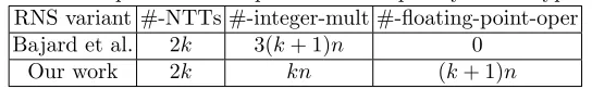
as used in our work, which implies we incrementedk0as needed when additional auxiliary moduli are introduced. Three main metrics are used to measure the complexity: number of NTTs, number of integer modular multiplications, and number of floating-point operations. While these metrics ignore regular modular reductions and modular additions/subtractions, the integer modular multiplica-tions are the dominant factor in CRT basis extension and scaling operamultiplica-tions in both variants.
Table 1: Comparison of computational complexity for decryption RNS variant #-NTTs #-integer-mult #-floating-point-oper
Bajard et al. 2k 3(k+ 1)n 0
Our work 2k kn (k+ 1)n
Table 2: Computational complexity for homomorphic multiplication
RNS variant #-NTT #-integer-mult #-floating-point-oper
Bajard et al.k2+ 9k+ 7k0+ 7 (21 + 10kk0+ 2k2+ 25k+ 28k0)n 0
Our work k2+ 9k+ 7k0 (10kk0+ 2k2+ 11k+ 14k0)n (7k+ 3k0+ 10)n
The number of NTTs in the decryption procedure is the same for both vari-ants, but Bajard et al. use three times as many integer modular multiplications (due to the operations using an auxiliary modulus). The extra cost that our variant has is (k+ 1)nfloating-point multiplications (either using double or ex-tended double precision). Our experiments indicate that this is faster than kn
have a lower runtime, which is confirmed by the experimental CPU and GPU results for both variants presented in [2].
We remark that Bajard et al. also discuss in Section 3.5 [3] a possible op-timization of their decryption procedure by using some floating-point precom-putations. However, even that optimized variant requires 2kn integer modular multiplications.8
Table 2 shows that the homomorphic multiplication procedures of both vari-ants have almost the same number of NTTs and same coefficients for quadratic
kk0 and k2 terms. However, the coefficients for the k, k0 and constant terms
are significantly larger in the Bajard et al. variant. For instance, when k = 5 the total number of integer multiplications for our variant is 489 n vs. 664 n
multiplications for the Bajard et al. variant, which is 26% less.
The higher numbers of integer modular multiplications in the Bajard et al. variant are caused by two auxiliary moduli introduced in the procedures. The profiling of our implementation code showed that the cost of floating-point op-erations in this case is much smaller than the cost of additional integer modular multiplications the Bajard et al. variant introduces. In other words, our homo-morphic multiplication procedure is expected to have a lower runtime, which is confirmed by the experimental CPU and GPU results for both variants pre-sented in [2]. More granular comparison of the computational complexity for both variants is presented in [2].
6
Implementation Details and Performance Results
6.1 Parameter Selection
Tighter heuristic (average-case) noise bounds. The polynomial multipli-cation expansion factor δ in Eqs. 8 and 9 is typically selected asδ=n for the worst-case scenario [3, 15]. However, our experiments for the textbook BFV, our BFV variant, and products of discrete Gaussian and ternary generated poly-nomials showed that we can select δ =C√n for practical experiments, where
C is a constant close to one (for the case of power-of-two cyclotomics). This follows from the Central Limit Theorem (or rather subgaussian analysis), since all dominant polynomial multiplication terms result from the multiplication of polynomials with zero-centered random coefficients.
The highest experimental value ofC for which we observed decryption fail-ures was 0.9. We also ran numerous experiments at nvarying from 210 to 217 for the cases of (1) multiplying a discrete Gaussian polynomial by a ternary uni-form polynomial and (2) multiplying a discrete uniuni-form polynomial by a ternary uniform polynomial, which cover the dominant terms in the noise constraints for BFV. The highest experimental value of C (observed for the product of a discrete Gaussian polynomial by a ternary uniform polynomial atn= 1024) was
8
1.75. In view of the above, we selected C = 2 for our experiments, i.e., we set
δ= 2√n.
Security. To choose the ring dimension n, we ran the LWE security esti-mator9 (commit f59326c) [1] to find the lowest security levels for the uSVP, decoding, and dual attacks following the standard homomorphic encryption se-curity recommendations [7]. We selected the least value of the number of sese-curity bitsλfor all 3 attacks on classical computers based on the estimates for the BKZ sieve reduction cost model.
The secret-key polynomials were generated using discrete ternary uniform distribution over{−1,0,1}n. In all of our experiments, we selected the minimum ciphertext modulus bitwidth that satisfied the correctness constraint for the lowest ring dimensionncorresponding to the security levelλ≥128.
Other parameters.We set the Gaussian distribution parameterσto 8/√2π
[7], the error boundBeto 6σ, and the lower bound forpto 2tnq. For the digit de-composition of residues in the relinearization procedure, we used the basewof 30 bits for the range of multiplicative depths from 1 to 10. For larger multiplicative depths, we utilized solely the CRT decomposition.
6.2 Implementation Details
Software Implementation.The BFV scheme based on the decryption and ho-momorphic multiplication algorithms described in this paper was implemented in PALISADE10, a modular C++11 lattice cryptography library that supports several SHE and proxy re-encryption schemes based on cyclotomic rings [19]. The results presented in this work were obtained for a power-of-two cyclotomic ringZ[x]/hxn+ 1i, which supports efficient polynomial multiplication using ne-gacylic convolution [16]. For efficient modular multiplication implementation in NTT, scaling, and CRT basis extension, we used the Number Theory Library (NTL)11 function
MulModPrecon, which is described in Lines 5-7 of Algo-rithm 2 in [13]. All single-precision integer computations were done in unsigned 64-bit integers. Floating-point computations were done in IEEE 754 double-precision and extended double-double-precision floating-point formats.
Our implementation of the BFV scheme is publicly accessible (included in PALISADE starting with version 1.1).
Loop parallelization. Multi-threading in our implementation is achieved via OpenMP12. The loop parallelization in the scaling and CRT basis extension operations is applied at the level of single-precision polynomial coefficients (w.r.t.
n). The loop parallelization for NTT and component-wise vector multiplications (polynomial multiplication in the evaluation representation) is applied at the level of CRT moduli (w.r.t.k).
9
https://bitbucket.org/malb/lwe-estimator 10https://git.njit.edu/palisade/PALISADE
11
http://www.shoup.net/ntl/ 12
Experimental setup.We ran the experiments in PALISADE version 1.1, which includes NTL version 10.5.0 and GMP version 6.1.2. The evaluation environment for the single-threaded experiments was a commodity desktop computer system with an Intel Core i7-3770 CPU with 4 cores rated at 3.40GHz and 16GB of memory, running Linux CentOS 7. The compiler was g++ (GCC) 5.3.1. The evaluation environment for the multi-threaded experiments was a server system with 2 sockets of 16-core Intel Xeon E5-2698 v3 at 2.30GHz CPU (which is a Haswell processor) and 250GB of RAM. The compiler was g++ (GCC) 4.8.5.
6.3 Results
Single-threaded mode. Table 3 presents the timing results for the range of multiplicative depthsLfrom 1 to 100 for the single-threaded mode of operation. It also demonstrates the contributions of CRT basis extension, scaling, and NTT to the homomorphic multiplication time (excluding the relinearization).
Table 3 suggests that the relative contribution of CRT basis extension and scaling operations to the homomorphic multiplication runtime (without relin-earization) first declines from 42% atL= 1 to 37% atL= 10, and then grows up to 50% at L = 100. The remaining execution time is dominated by NTT operations. Our complexity and profiling analysis indicated that the initial de-cline is caused by a decreasing contribution (w.r.t. to modular multiplications in NTTs) of the linear terms ofkandk0 to the computational complexity of homo-morphic multiplication askincreases from 1 to 4 (see Table 2). The subsequent increase in relative execution time is due to theO(k2n) modular multiplications needed for CRT basis extension and scaling operations, which start contributing more than the O(knlogn) modular multiplications in the NTT operations for polynomial multiplications ask further increases.
Our profiling analysis showed that the contributions of floating-point opera-tions to CRT basis extension and scaling were always under 5% and 10% (under 5% fork >5), respectively. This corresponded to at most 2.5% of the total ho-momorphic multiplication time (typically the value was closer to 1%). This result justifies the practical use of our much simpler algorithms, as compared to [3], considering that our approach has lower computational complexity (significantly more than by 5%, as shown in Section 5.2).
Table 3 also shows that the contribution of the relinearization procedure to the total homomorphic multiplication time grows from 11% (L = 1) to 57% (L = 100) due to the quadratic dependence of the number of NTTs in the relinearization procedure on the number of coprime modulik.
The profiling of the decryption operation showed that only 8% (L = 100) to 18% (L = 1) was spent on CRT scaling while at least 60% was consumed by NTT operations and up to 10% by component-wise vector products. This supports our analysis, asserting that the decryption operation is dominated by NTT, and the effect of the scaling operation is insignificant.
Table 3: Timing results for decryption, homomorphic multiplication, and relin-earization in the single-threaded mode; t= 2, log2qi≈55,λ≥128
L n log2q k Dec. [ms] Mul. [ms] Relin. [ms] Multiplication [%] CRT ext. Scaling NTT
1 211 55 1 0.15 3.16 0.41 34 8 52
5 212 110 2 0.49 10.1 2.58 29 9 56
10 213 220 4 1.89 38.9 18.7 27 10 56
20 214 440 8 8.3 174 78.3 27 14 54
30 215 605 11 25.8 555 332 27 15 52
50 216 1,045 19 95.8 2,368 2,066 30 20 46
100 217 2,090 38 409 12,890 16,994 30 20 46
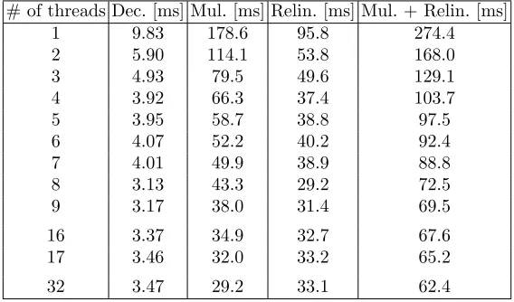
Table 4: Timing results with multiple threads for decryption, multiplication, and relinearization, for the case of L= 20, n= 214, k= 8 from Table 3
# of threads Dec. [ms] Mul. [ms] Relin. [ms] Mul. + Relin. [ms]
1 9.83 178.6 95.8 274.4
2 5.90 114.1 53.8 168.0
3 4.93 79.5 49.6 129.1
4 3.92 66.3 37.4 103.7
5 3.95 58.7 38.8 97.5
6 4.07 52.2 40.2 92.4
7 4.01 49.9 38.9 88.8
8 3.13 43.3 29.2 72.5
9 3.17 38.0 31.4 69.5
16 3.37 34.9 32.7 67.6
17 3.46 32.0 33.2 65.2
32 3.47 29.2 33.1 62.4
runtime improvement factors for decryption and homomorphic multiplication (with relinearization) are 3.1 and 4.4, respectively.
The decryption runtime is dominated by NTT, and the NTTs are paral-lelized at the level of CRT moduli (parameter k, which is 8 in this case). Ta-ble 4 shows that the maximum improvement is indeed achieved at 8 threads. Any further increase in the number of threads increases the overhead related to multi-threading without providing any improvement in speed. The theoretical maximum improvement factor of 8 is not reached most likely due to the distri-bution of the load between the cores of two sockets in the server. A more careful fine-tuning of OpenMP thread affinity settings would be needed to achieve a higher improvement factor, which is beyond the scope of this work.
scaling operations, which are parallelized at the level of polynomial coefficients (parameter n = 214). However, as the contribution of NTT operations is high (nearly 70% for the single-threaded mode, as illustrated in Table 3), the bene-fits of parallelization due to CRT basis extension and scaling are limited (their relative contribution becomes smaller as the number of threads increases).
The relinearization procedure is NTT-bound and, therefore, shows approxi-mately the same relative improvement as the decryption procedure, i.e., a factor of 2.9, which reaches its maximum value at 8 threads.
In summary, our analysis suggests that the proposed CRT basis extension and scaling operations parallelize well (w.r.t. ring dimension n) but the over-all parover-allelization improvements of homomorphic multiplication and decryption largely depend on the parallelization of NTT operations. In our implementa-tion, no intra-NTT parallelization was applied and thus the overall benefits of parallelization were limited.
7
Conclusion
In this work we described simpler alternatives to the CRT basis extension and scaling procedures of Bajard et al. [3], and implemented them in the PALISADE library [18]. These procedures are based on the use of floating-point arithmetic for certain intermediate computations. Our analysis demonstrates that these procedures are not only simpler, but also have lower computational complexity and noise growth than the procedures proposed in [3].
Our single-threaded and multi-threaded experiments suggest that the main bottleneck of the implementation of our BFV variant is the NTT operations. In other words, the cost of the CRT maintenance procedures, i.e., CRT basis extension and scaling, is relatively small. Therefore, further impovements in the BFV runtimes can be achieved by optimizing the NTT operations, focusing on their parallelization.
We have shown that our procedures can be applied to any scale-invariant homomorphic encryption scheme based on the original Brakerski’s scheme, in-cluding YASHE. The CRT basis extension and scaling procedures may also be utilized in other lattice-based cryptographic constructions; for instance, scaling is a common technique used in many lattice schemes based on dual Regev’s cryptosystem [11, 20].
References
1. Albrecht, M., Scott, S., Player, R.: On the concrete hardness of learning with errors. Journal of Mathematical Cryptology 9(3), 169–203 (10 2015)
2. Badawi, A.A., Polyakov, Y., Aung, K.M.M., Veeravalli, B., Rohloff, K.: Compari-son and evaluation of rns variants of the bfv homomorphic encryption scheme, in preparation, (Personal communication), 2018
4. Bos, J.W., Lauter, K., Loftus, J., Naehrig, M.: Improved security for a ring-based fully homomorphic encryption scheme. In: IMACC 2013. pp. 45–64 (2013)
5. Brakerski, Z.: Fully homomorphic encryption without modulus switching from clas-sical gapsvp. In: CRYPTO 2012 - Volume 7417. pp. 868–886 (2012)
6. Brakerski, Z., Gentry, C., Vaikuntanathan, V.: (leveled) fully homomorphic en-cryption without bootstrapping. In: ITCS ’12. pp. 309–325 (2012)
7. Chase, M., Chen, H., Ding, J., Goldwasser, S., Gorbunov, S., Hoffstein, J., Lauter, K., Lokam, S., Moody, D., Morrison, T., Sahai, A., Vaikuntanathan, V.: Security of homomorphic encryption. Tech. rep., HomomorphicEncryption.org, Redmond WA (July 2017)
8. Fan, J., Vercauteren, F.: Somewhat practical fully homomorphic encryption. Cryp-tology ePrint Archive, Report 2012/144 (2012)
9. Gentry, C.: Fully homomorphic encryption using ideal lattices. In: STOC ’09. pp. 169–178 (2009)
10. Gentry, C., Halevi, S., Smart, N.: Homomorphic evaluation of the AES circuit. In: ”CRYPTO 2012”. LNCS, vol. 7417, pp. 850–867 (2012)
11. Gentry, C., Peikert, C., Vaikuntanathan, V.: Trapdoors for hard lattices and new cryptographic constructions. In: Proceedings of the Fortieth Annual ACM Sym-posium on Theory of Computing. pp. 197–206. STOC ’08, ACM, New York, NY, USA (2008),http://doi.acm.org/10.1145/1374376.1374407
12. Halevi, S., Shoup, V.: Design and implementation of a homomorphic-encryption library.https://shaih.github.io/pubs/he-library.pdf(2013)
13. Harvey, D.: Faster arithmetic for number-theoretic transforms. Journal of Symbolic Computation 60, 113 – 119 (2014)
14. Kawamura, S., Koike, M., Sano, F., Shimbo, A.: Cox-rower architecture for fast parallel montgomery multiplication. In: EUROCRYPT 2000. pp. 523–538 (2000)
15. Lepoint, T., Naehrig, M.: A comparison of the homomorphic encryption schemes fv and yashe. In: AFRICACRYPT 2014. pp. 318–335 (2014)
16. Longa, P., Naehrig, M.: Speeding up the number theoretic transform for faster ideal lattice-based cryptography. In: Foresti, S., Persiano, G. (eds.) Cryptology and Network Security. pp. 124–139. Springer International Publishing, Cham (2016)
17. Lyubashevsky, V., Peikert, C., Regev, O.: A toolkit for ring-lwe cryptography. In: Johansson, T., Nguyen, P.Q. (eds.) EUROCRYPT 2013. pp. 35–54 (2013)
18. Polyakov, Y., Rohloff, K., Ryan, G.W.: PALISADE lattice cryptography library.
https://git.njit.edu/palisade/PALISADE(Accessed January 2018)
19. Polyakov, Y., Rohloff, K., Sahu, G., Vaikuntanathan, V.: Fast proxy re-encryption for publish/subscribe systems. ACM Trans. Priv. Secur. 20(4), 14:1–14:31 (2017)
20. Regev, O.: On lattices, learning with errors, random linear codes, and cryptog-raphy. In: Proceedings of the Thirty-seventh Annual ACM Symposium on The-ory of Computing. pp. 84–93. STOC ’05, ACM, New York, NY, USA (2005),
http://doi.acm.org/10.1145/1060590.1060603
21. Regev, O.: On lattices, learning with errors, random linear codes, and cryptogra-phy. J. ACM 56(6) (2009)
A
Appendices
A.1 Alternative variant of complex scaling in CRT representation
This section presents an alternative variant of complex scaling in CRT represen-tation. This variant has a reduced size requirement forp(by a factor oft) and very similar computational complexity.
The input isx∈Zqp, represented in the CRT basis{q1, . . . , qk, p1, . . . , pk0}. We need to scale it byt/q and round, and we want the result modulo qin the CRT basis{q1, . . . , qk}. Namely, we want to compute
dt/q·xc
qi for alli. We combine techniques from the procedures in Sections 2.2 and 2.3, computing the ratioυ as in Section 2.2, then computing Eq. 3 modulo each of theqi’s similarly to Section 2.3. Let us denote:Q:=qp, Q∗i :=Q/qi=qi∗p, Q0j
∗
:=Q/pj =qp∗j, and also ˜Qi= [(Q∗i)−1]qi and ˜Q0j = [(Q0j
∗
)−1]
pj. Then by Eq. 3 we have
t
q ·x=
t q
k
X
i=1
[xiQ˜i]qiQ∗i + k0
X
j=1 [x0jQ˜0
j]pjQ0j
∗ −υQ = k X i=1
[xiQ˜i]qi·tp/qi+ k0
X
j=1 [x0jQ˜0
j]pj·tp∗j−υtp, (14)
and the ratioυis computed as
υ=
& Pk
i=1[xiQ˜i]qiQ∗i +
Pk0
j=1[x
0
jQ˜0j]pjQ0j
∗ Q % = k X i=1
[xiQ˜i]qi
qi +
k0
X
j=1 [x0jQ˜0
j]pj
pj
.
We thus computeyi:= [xiQ˜i]qi andzi=yi/qi for alli, andy
0
j:= [x0jQ˜0j]pj and
zj0 =y0j/pj for allj, and setυ:=
l P
izi+Pjzj0
k
.
As in Section 2.3, we pre-compute all the values tp/qiq
i , breaking them into their integral and fractional parts,tpq
i =ω
0
i+θ0iwithω0i∈Ztpandθi0∈[− 1 2,
1 2). We store all theθ0i’s as double floats, and for everyi, i0 we store the single-precision integer ωi,i0 0 = [ωi00]qi. In addition, and for everyi, j we storeζi,j = [tp∗j]qi, and for everyi we storeλj:= [tp]qi.
On inputs (x1, . . . , xk, x01, . . . , x0k0) we compute υand all the yi’s andyj0’s as above, then compute Eq. 14 modulo each of theqi’s, by setting
v0 :=dP
iθ
0
iyic, and for alli w0i:=
P
i0yi0ω0
i,i0+Pjy0jζi,j+υλj
qi.
The complex scaling procedure returns [dt/q·xc]qi = [v
0+w0
i]qi for alli.
Correctness.The correctness details are essentially the same as for the complex scaling in Section 2.4.
k+ 1 more floating-point operations, and computing each w0i takes k+k0+ 1 modular multiplications. In total, complex CRT scaling therefore takes 2k+
k0+ 2 floating point operations andkk0+k2+ 2k+k0 single-precision modular