Victoria University of Technology
Department of Electrical & Electronic Engineering
T 4 ^
2.
COGENERATION IN DISTRIBUTION SYSTEM:
PLANNING, OPERATION AND TRANSIENTS
Mahavir Singh
B.Sc. Honours, B.Sc. (Engg.), M . S .
The work presented in this thesis was carried out under the
supervision of Associate Professor Dr Akhtar Kalam, B.Sc, B.Sc.
(Engg.), M.S., Ph.D. of the Department of Electrical and
Electronincs Engineering, Victoria University of Technology,
Footscray. His guidance, assistance and encouragement from the
campus office as well as from overseas is highly appreciated. The
project was started at the Royal Melbourne Institute of
Technology under the supervision of Dr. Majid Al-Dabbagh to whom
I thank very much. I had to make a few trips to Sydney in the
initial phase of the project to consult Dr. Don Geddy, Planning
and Development Engineer, at the Electricity Commission of New
South Wales, to use the EMTP software. I thank him for offering
his valuable experience in this field.
To make the project more meaningful to the electrical industry,
I consulted Mr. Bob Coulter, Distribution Engineer at the State
Electricity Commission of Victoria, very often. His advice and
assistance have made this project valuable to electrical
industry. I thank him for all the time spent for this project. I
also thank Mrs Ann Pleasant, Senior Lecturer, who assisted me
during the period of Dr. Kalam's absence.
The technical staff of the University have been helpful whenever
problems with the functioning of the computer and software came
up. Mr Neil Larchin, Mr Zoltan Varga and Mr Foster Hayward were
of Protel and Word Perfect softwares. I acknowledge their
LIST OF CONTENTS page SUMMARY CHAPTER 1 1.1 1.2 INTRODUCTION Literature Survey Aims of the Thesis
1 4 4 30 CHAPTER 2.0 2 2 2 2 2 2 .1 2 ,3 .4 .5 .6 2.7 2.8 CHAPTER 3 3.0 3.1 3.2 3.3 CHAPTER 4 4.0 4.1 4.2 4.3 4.4 4.5 4.6 4.7 4.8
MATHEMATICAL MODELLING 33
Introduction 33 The solution of transient phenomena 33
Single phase network 34 Branch equations 35 Nodal equations 41 Practical computation 43
Extension to multi-phase network 44 2.6.1 Lumped parameters with mutual couplings 44
Switches 47 Positive and zero sequence parameters of
single-circuit three-phase lines 49 CIRCUIT PARAMETERS 52
Introduction 52 Line impedance and formation of Pi-models 53
Computation procedure 54 3.2.1 Computation of line parameters 54
Format for entering the line parameters 61 ABNORMAL CONDITIONS: GRAPHICAL OUTPUTS 64
Introduction 64 Abnormalities at various points when ground
fault occurs at SYSTA 64 Abnormalities at various points when 2-phase
to ground fault occurs at P191 67 Abnormalities at various points when two phases
form short circuit on the generator's terminals and simultaneously open circuit on the load
side 69 Abnormalities at various points when a broken
conductor fault occurs at P191: induction
generator side of break contacting ground 70 Abnormalities at various points when a broken
conductor fault occurs at P191: system side of
break contacting ground 71 Abnormalities at different points of a feeder
when the generator is disconncted at the
terminal by an ideal three phase device 73 Abnormalities at different points of the feeder
when the generator is switched on to it by an
ideal three phase device 76 Abnormalities at different points of the feeder
supply system 78
CHAPTER 5
-5.0 5.1 5.2 5.3 5.4 5.5 5.6 5.7 5.8 5.9 5.10 5.11 5.12 5.13 5.14
PLANNING AND OPERATION OF DISTRIBUTION CIRCUITS
WITH DISPERSED STORAGE GENERATION 80
Introduction 80 Delivery system characteristics 80
5.1.1 Reserve capacity 80 5.1.2 Distribution reliability 81
5.1.3 Distribution losses 82 5.1.4 Radial operation 82 5.1.5 Thermal and voltage limitations 82
Distribution planning characteristics 83
5.2.1 Planning for peak load 83 5.2.2 Planning objectives 83 5.2.3 Planning criteria 84 5.2.4 Voltage and current criteria 85
Planning for normal and emergency conditions 86
5.3.1 Use of judgement and experience 86
5.3.2 Adoption of new technology 87
5.3.3 Planning horizon 87 Characteristics common to storage & generation 88
5.4.1 Impact on generation 88 5.4.2 Economy of scale capital cost 89
5.4.3 Operation and maintenance 89
Communications and Control 89
Interface 90 Reliability 90 Planning and operation with DSG 90
5.8.1 Supply-side device 90 5.8.2 Customer-side device 93
Interconnection 94 Power quality 95
5.10.1 Power factor correction 96 5.10.2 Voltage regulation 9 8
5.10.3 Harmonic distortion 101
5.10.4 Earthing 103 Protection of cogenerator's plant 106
Supply network interconnection circuits 107 5.12.1 Interconnection circuit protection
requirements 107 5.12.2 Autoreclose 110 5.12.3 Islanding operation 110
5.12.4 Supply network protection requirements
to allow for private generation 112
5.12.5 Customer plant protection 112
Safety 112 Metering 115 CHAPTER - 6 CONCLUSIONS AND FUTURE WORK
6.0 Introduction 6.1 Conclusions 6 .2 Future work
Fig. Fig. Fig. Fig. Fig. Fig. Fig. Fig. Fig. Fig. Fig. Fig. Fig. Fig. Fig. Fig. Fig. Fig.
2-1 2-2 2-3 2-4 2-5 2-6
2-7 2-8 3-1 4-1 4-1A 4-2 4-3 4-4
4-5
4-6
4-7
4-8
LIST OF FIGURES
Single-phase network 34
Equivalent circuit for lossless lines 37
Trapezoidal rule for integration 39 Equivalent circuit for inductance 39 Equivalent circuit for capacitance 41
Solving linear equations with changing right
side 43 Coupled R-L branches 45
Triangularization in two steps 48 Distribution circuit of SECV 52
Ground fault at SYSTA 64 Current flow during fault at SYSTA 66
Double line-to-ground fault 67 Phase to phase short circuit 69
Broken conductor at P191; induction generator
side of break grounded 70 Broken conductor at P191; system side of break
grounded 71 Generator disconnected at terminals of ideal
3-phase three phase switching device 73 Generator energisation: terminals of ideal
3-phase switching device closed 76
List of Principal Symbols
Instantaneous voltage at time t 33
Instantaneous current at time t 33 Very small interval of time 33
Instantaneous current entering node 1 34 Instantaneous current flowing from node 1
to node 2 34 Instantaneous current flowing from node 1
to node 3 35 Instantaneous current flowing from node 1
to node 4 35 Instantaneous current flowing from node 1
to node 5 35 Current entering node 1 at time t 35
Current between nodes 1 and 2 at time t 35 Current between nodes 1 and 3 at time t 35 Current between nodes 1 and 4 at time t 35
Current between nodes 1 and 5 at time t 35
Instantaneous voltage at distance x and time t 35
Inductace per unit length 35 Capacitance per unit length 35
Distance on the line from some arbitrary
chosen point 35 Propagation velocity 36
Time taken by a wave to travel from one
end of line to the other 37 Impedance of a line from one node to ground 3 8
Nodal admittance matrix 41 Column vector of n node voltages at time t 41
Column vector of n injected node currents at
time t 41 Constant column vector 41
Transformation matrix 49
Subscripts
Phases A, B and C
Self and mutual impedances
Zero, alpha and beta components
Zero value component of symmetrical components Positive value component of symmetrical
components
List Of Abbreviations
DSG PURPA NEAC FERC QF NGPA FUA CAA NAAQS PDS NSPS EPA LAER NEPA OSHA NECPA NPDES
IOU ITC COP AGC ATP DSSG DCSG PCC EPRI APPA
Dispersed storage and generation 5 Public Utility Regulatory Act 6 National Energy Advisory Committee 9
Federal Energy Regulatory Commission 10 Qualifying (cogeneration) facility 10
Natural Gas Policy Act 15
Fuel Use Act 15 Clean Air Act 17 National Ambient Air Quality Air Standards 17
Prevention Of Significant Deterioration 17
New Source Performance Standards 17 Environmental Protection Agency 18 Lowest Achievable Emission Rate 18 National Environment Policy Act 19 Occupational Service and Health Administration 19
National Energy Conservation Policy Act 19 National Pollution Discharge Elimination System 19
Investor-owned Utility 23 Investments Tax Credits 24 Current Operational Problems 27
Automatic Generation Control 28 Alternative Transient Program 31 Dispersed Supply-Side Storage and Generation 90
Dispersed Customer Side Generation 93
Point Of Common coupling 102 Electric Power Research Institute 102
Summary
Since the oil crisis of 1970's there has been an increasing
awareness of the need for energy efficiency and sufficiency.
Australia is also alert of the energy economy. The National
Advisory Committee recommended in 1983 that the Commonwealth should
urge the state governments to encourage the electricity supply
authorities to "facilitate greater use in the grid of privately
generated electricity" [68]. This law opened an opportunity for the
use of private generators, which had been on standby duties for use
only in emergency. They could become suppliers of electricity
without having to install transmission lines and other components.
Other dispersed sources which produce electric energy from
hydrogenerators, wind turbines, biomass, waste and other
non-conventional sources, could also be business partners of the
utility. These DSGs (dispersed storage and generation) are allowed
to use the transmission facilities built by the utility. The issue
has gained so much momentum that Bates says, "In this respect we
are totally at odds with the Industry Commission, which recommended
the breaking-up of the State Electricity utilities by the wholesale
selling-off of generating and distribution assets to the private
sector" [67].
This thesis relates to a study of abnormal conditions on a
Commission of Victoria (SECV) with several loads and a capacitor
bank. An induction generator, which plays the role of a dispersed
storage and generation unit, driven by a hydraulic turbine, which
is a common form of renewable energy scheme, is connected to the
distribution feeder through a A/Y transformer. Transients caused by
switching of the induction generator, by single line-to-ground
fault, double line-to-ground fault through contact resistances,
broken conductor touching the ground through a small resistance,
isolating the induction generator to form its own supply domain
(islanding) etc are investigated and interesting conclusions of
practical importance are derived.
The IBM PC version 4 of the ElectroMagneticTransient Program
-Alternative Transient Program (ATP), was used to solve this
problem. The program also gives output results for automatic
plotting in time domain. Accordingly, transient voltages at several
nodes and transient currents at interesting points were plotted
from the output results.
Planning and operational aspects like voltage control, reliability,
harmonics, earthing, and contractual matters between the private
generator and the utility are also considered. Technical aspects of
interconnections between the private generation and the utility has
been considered.
interrupting duty on circuit breakers, effect on response of
protective relays and automatic control systems are pointed out. It
also considers security to personnel and protection of metering
equipment. The thesis also offers guide for contractual matters
CHAPTER 1 INTRODUCTION
1.1 Literature Survey
If an induction motor is driven by an outside mechanical source
at speeds above synchronism, the power current component in the
stator reverses while the magnetising component remains in
magnitude and phase position. The machine thus is converted to
a generator, referred to as induction generator, and will deliver
active power when its shaft input has overcome its internal
losses. Induction generators are relatively smaller in sizes than
synchronous alternators; for although they supply active power,
they take reactive current from other synchronous machines. In
other words, irrespective of load conditions, the induction
generator must operate at leading power factor. The driving force
for the generator can be supplied by a low speed water turbine
or by high-speed steam and gas turbines. Induction generators in
combination with switched capacitor banks can be used in
relatively large-scale installations, provided they are tied to
a transmission network, at least partly supplied by synchronous
alternators to maintain frequency.
The West 59th Street power house of the Interborough Rapid
7500-kW exhaust turbine induction generator sets which operate
from the steam discharged by five 7500-kW 25-cycle
angle-compounded steam-engine alternators. This increased the
thermal efficiency of the plant and doubled its output. A large
number of induction motors were converted to induction generators
during World War II because of the limitations of power usage and
availability of induction motors as compared to synchronous
alternators [69].
Dispersed storage and generation (DSG) is an expression coined
by the Institute of Electrical & Electronic Engineers in an
attempt to clear up the semantic confusion between
interconnection and cogeneration [10]. DSG is also used by some
authors for the abbreviation of Distribution System Generation
[18] . The SECV uses the expression "Private generation" in place
of DSG [64] . They all give the same idea of generating
electricity from sources like wind power, water power, solar
power and bio-gas (obtained from agricultural digester) . DSGs may
be defined as any source of electrical energy (including storage
elements which act as sources at times) connected directly to a
utility distribution system or sub-transmission system.
The class of devices which comprise the DSGs are listed below
[5]':
* Hydroelectric
* Solar Thermal Electric
* Wind
* Storage Battery
* Hydroelectric Pumped storage
* Cogeneration
Among these cogeneration has become very important and
interesting too.
Since 1973 the oil embargo and the energy crisis generated by
that embargo, there has been much concern expressed over ways to
conserve and use energy more efficiently. One area of specific
investigation is cogeneration. The Public Utility Regulatory
Policy Act (PURPA) defines cogeneration as the production of
electric energy and other useful energy (such as heat), which are
used for industrial, commercial, heating, or cooling purposes
[70] .
Cogeneration is the combined production of two forms of energy,
electrical or mechanical power plus thermal energy, in one
technological process. The electrical power produced by a
cogenerator can be used on site or distributed through the
utility grid, or both. The thermal energy usually is used on site
for industrial process heat or steam, space conditioning, and/or
hot water. But, if the cogeneration system produces more useful
thermal energy than is needed on site, distribution of the excess
to nearby facilities can substantially improve the cogenerator's
The total amount of fuel needed to produce both electricity and
thermal energy in a cogenerator is less than the total fuel
needed to produce the same amount of electric and thermal energy
in separate technologies. It is primarily this greater fuel use
efficiency that has created a resurgence of interest in
cogeneration systems. However, cogeneration also can be
attractive as a means of adding electric generating capacity
rapidly at sites where thermal energy already is produced.
Cogeneration systems recapture otherwise wasted thermal energy,
usually from a heat engine producing electric power, and use it
for applications such as space heating, industrial process needs,
or water heating, or use it as an energy source for another
system component. This "cascading" of energy use is what
distinguishes cogeneration systems from conventional separate
electric and thermal energy system. Thus, conventional energy
systems supply either electricity or thermal energy while a
cogeneration system produces both.
Cogeneration technologies are termed "topping cycles" if the
electric or mechanical power is produced first, and the thermal
energy exhausted from power production is then captured and used.
"Bottoming cycle" cogeneration systems produce high-temperature
thermal energy first and then recover the waste heat for use in
generating electric or mechanical power plus additional, lower
temperature thermal energy.
Energy". In the late 1950's and early 1960's the "total energy"
concept was promoted by many of the gas companies and some
equipment suppliers [6-9].
Early in this century, at the time when electricity first became
widely used, many large industrial or commercial enterprises
maintained large steam boiler plants for space heating and/or
process heating. It was relatively an easy matter to boost the
boiler steam pressure somewhat beyond the process requirement,
insert a turbine which was connected to an electric generator,
and then use the steam for its original requirement after the
added energy was extracted to generate electricity. It was a
practical concept at that time [6] . The gas companies had
tremendous quantities of natural gas and this concept created an
almost constant demand for the natural gas to operate a
combustion turbine or gas-fired engine which produced the
electric energy required by the facility, and as a by-product,
the exhaust could be used to produce process heating or cooling.
The weak point in the total energy installation was that, for
economic reasons, the electrical demand curve had to coincide
with the heat energy [19-21].
The electric utilities did not want to lose their revenue. They
argued against the weak aspect of the total energy installations
and challenged the concept as uneconomical because of poor load
balance. The maintenance required for high reliability was very
costly and the supply of natural gas became very tight in 1971.
Herein, lies the difference between the total energy and
cogeneration. The appeal of the total energy was based on
complete independence from the electric utility and the utilities
fought it. Cogeneration as presently conceived, however, is based
on both parties participating in, and sharing the benefits of,
cogeneration and has received utility endorsement [6].
Between the late 1880's and early 1900's oil-and-gas-fired
cogeneration technologies were increasingly used throughout
Europe and the United States. In 1900, over 59 percent of total
U.S. electric generating capacity was located at industrial sites
[22-27] .
There has been a resurgence of interest in recent years in
cogeneration for industrial sites, commercial buildings, and
rural applications. In Australia, the National Energy Advisory
Committee (NEAC) recommended in 19 83 that the Commonwealth should
advise the state governments to encourage the electricity supply
authorities to permit the private generators to use their grid
[68] . In the U.S.A. cogenerators faced three major obstacles when
seeking interconnected operation with an electric utility. First,
utilities were often reluctant to purchase cogenerated
electricity at a rate that made interconnected cogeneration
economically feasible. Second, some utilities charged very high
rates for providing backup service to cogenerators. Third, a
cogenerator that sold electricity risked being classified as an
electric utility and was expected to be regulated under State and
cogeneration was not able to compete with electricity generated
in central station power plants.
A number of recent legislative initiatives are intended to
clarify the role of cogeneration within national energy and
environmental policy, and to encourage its use under those
circumstances, where it would save fuel or allow increased
efficiency in electric utilities' use of facilities and
resources. Utilities are required to purchase electricity from,
and provide backup service to cogenerators and at rates that are
just and reasonable, that are in the public interest, and that
do not discriminate against cogenerators. PURPA also allows
Federal Energy Regulatory Commission (FERC) to exempt
cogenerators from state regulation of utility rates and
financial organisation, and from Federal regulations under the
Federal and Public Utility Act [93-95].
"Qualifying cogeneration facility" (QF) is defined as one that
produces electricity and steam or other forms of useful thermal
energy for industrial, commercial, heating, or cooling purposes;
that meets the operating requirements prescribed by the
government. Electric utilities are also required to interconnect
with QF and must offer to operate in parallel with them.
Cogenerators must meet the operating requirements to qualify for
interconnections and other benefits.
An electric utility can participate in the ownership of a
company. Efficiency and operating standards are also prescribed
in the rules to distinguish bonafide cogenerators from
essentially single purpose facilities. This standard specifies
that at least 5% of a "topping cycle" cogenerator's total energy
output (on an annual basis) must be useful thermal energy. This
"topping cycle" efficiency standard is designed to ensure that
an oil or natural-gas-fired cogenerator will use these fuels more
efficiently than any combination of separately generated
electric and thermal energy using efficient state-of-the-art
technology. "Topping cycle" cogenerators that were installed
prior to 19 80, and those that use fuels other than oil and gas
do not have to meet any efficiency standards in order to qualify
under PURPA [71].
The 2-to-l weighting in favour of electricity production in these
"topping cycle" efficiency standards reflects the view that
systems with high electricity to heat ratios have the highest
energy efficiencies and their development and use should be
encouraged [96]. This weighting will be more equitable to the
various cogeneration technologies than a standard that simply
summed electric and thermal output on an equal basis, because the
latter would have made it relatively easy for steam turbines that
produce little electricity to qualify, but would have penalised
higher electricity-to-steam ratio systems through difficult heat
recovery requirements.
In this context "Avoided Cost" has been defined as the
capacity or both, which but for the purchase from a cogenerator
or small power producer, the utility would generate itself or
purchase from another source. The rules impose electric utilities
an obligation to purchase all electric energy and capacity made
available from a QF with which the electric utility is directly
or indirectly interconnected, except during system emergencies
or during light load periods. PURPA specifies that purchase power
rates must be just and reasonable to the electric utilities'
consumers and in the public interest, and must not exceed the
avoided cost to the utility of alternative electric energy.
"Capacity costs" are the costs associated with providing the
capability to deliver energy; they consist primarily of the
capital costs of generating and other facilities [72]. The energy
costs as aforementioned are the variable costs associated with
the production of electricity, and include the cost of fuel and
some operating and maintenance expenses. Thus, if by purchasing
electricity, from a qualifying facility, a utility can reduce its
energy costs or can avoid purchasing energy from another utility,
the rate for the purchase from the QF must be based on those
energy costs that the utility can thereby avoid. Similarly, if
the QF offers energy of sufficient reliability and guarantees of
deliverability to permit the purchasing utility to build a
smaller, less expensive plant, avoid the need to construct -a
generating unit, or reduce firm power from the grid, then the
purchase rates must be based on both the avoided capacity and
energy costs [72]. In each case, it is the incremental costs, and
There is a provision in the rules that a utility that receives
energy or capacity from a QF may, with the consent of the QF,
transmit that energy or capacity to a second utility. However,
if the QF does not consent to transmission to another utility,
the local utility retains the purchase obligation. Similarly, if
the local utility does not agree to transmit the QF's energy or
capacity, it retains the purchase obligation. Because the
transmission can only occur with the consent of the utility to
which the energy or capacity is first delivered, this rule does
not force wheeling of power [72].
The rule on transmission of cogenerated power specifies that any
electric utility to which such energy or capacity is delivered
must purchase that energy or capacity under the same obligations
and at the same rates as if the purchase were made directly from
the QF. These rates should take into account any transmission
losses or gains. If the electricity from the QF actually travels
across the transmitting utility's system, the amount of energy
delivered will be less than that transmitted, due to line losses,
and the purchase rate should reflect these losses [73].
Section 210(a) of PURPA also requires that each electric utility
offer to sell electric energy to a QF. This obligation to sell
power is interpreted as requiring utilities to provide four
classes of service to QF's [46, 58-60]:
(a) "Supplementary Power", which is energy or capacity used
(b) "Interruptable Power", which is energy or capacity that
is subject to interruption by the utility under
specified conditions, and is normally provided at a
lower rate than non-interruptable service if it
enables the utility to reduce peak loads
(c) "Maintenance Power", which is energy or capacity
supplied during scheduled outages of the QF,
presumably during periods when the utility's other
load is low
(d) "Backup Power", which is the energy or capacity supplied
during unscheduled outages
A utility may avoid providing any of these four classes of
service only if it convinces the Public Service Commission that
compliance would impair its ability to render adequate service
or would place an undue burden on the electric utility [74].
Interconnection costs must be assessed on a
non-discriminatory-basis with respect to non-cogenerating customers with similar
load characteristics, and may not duplicate any costs including
the avoided costs [75]. Standard or class charges for
interconnection may be included in purchase power tariffs for QFs
with a design capacity of 100 kW or less, and Public Service
Commissions may also determine interconnection costs for larger
facilities on either a class or individual basis.
Cogenerators' fuel choice may be influenced by the Fuel Use Act
pricing rules of Natural Gas Policy Act of 1978 (NGPA), as well
as by the environmental requirements and tax incentives.
A cogenerator may be subject to the FUA prohibitions if it has
a fuel heat input rate 100 of million Btu per hour or greater and
if it comes within the statutory definition of either a power
plant or a major fuel-burning installation. Under FUA, a power
plant includes "any stationary electric generating unit",
consisting of a boiler, a gas turbine, or a combined-cycle unit
that produces electric power for purposes of sale or exchange",
but does not include cogeneration facilities if less than half
of the annual electric output is sold or exchanged for resale.
A major fuel-burning installation is defined as "a stationary
unit consisting of a boiler, gas turbine unit, combined cycle
unit or internal combustion engine". However, the prohibition
against the use of oil and gas in new major fuel-burning
installations applies only to boilers.
FUA allows a permanent exemption for cogenerators for if the
"economic and other benefits of cogeneration are unobtainable
unless petroleum or other gas, or both, are used in such
facilities". The Department of Energy interprets the phrase
"economic and other benefits" to mean that the oil or gas to be
consumed by the cogenerator will be less than that which would
otherwise be consumed by the conventional separate electric and
thermal energy systems. Alternatively, if the cogenerator can
show that the exemption would be in the public interest (e.g.,
maintain employment in an urban area), the Department of Energy
will not require a demonstration of oil/gas savings [73]. The
regulation to implement the cogeneration exemption are subject
to change; therefore, it is uncertain how difficult it could be
to meet the exemption requirements, and thus how FUA will affect
the market penetration [75] .
Although the permanent exemption for cogeneration is likely to
be the preferred route for potential cogenerators subject to the
FUA prohibitions, several other exemptions may be applicable in
certain circumstances. First, a permanent exemption is available
to petitioners who propose to use a mixture of natural gas or
petroleum and alternate fuel. Under this mixtures exemption, the
amount of oil or gas to be used cannot exceed the minimum
percentage of the total annual Btu heat input of the primary
energy source needed to maintain operational reliability of the
unit consistent with maintaining a reasonable level of fuel
efficiency. Second, a temporary exemption is available to
petitioners who plan to use a synthetic fuel (derived from coal
or another fuel) by the end of the exemption period. Third, a
temporary public interest exemption may be obtained when the
petitioner is unable to comply with FUA immediately (but will be
able to comply by the end of the exemption) . One of the cases
where this public interest exemption may be granted is for the
use of oil or gas in an existing facility during the ongoing
construction of an alternate fuel-fired unit [63-66, 76].
its incremental pricing provisions to qualify cogeneration
facilities under PURPA. Thus, the potential lower gas prices
should not affect the relative competitiveness of gas-fired
cogeneration significantly. Moreover, plants burning intrastate
gas may not realise any savings because the fuel price is often
at the same level as the incremental price. In addition, the
deregulation could largely remove incremental pricing. These
uncertainties mean NGPA probably will not be a major factor in
cogeneration investment decisions [77] .
Cogeneration can have significant impacts on air quality,
especially in urban areas. Depending on cogenerator's size and
location, it may be subject to one or more of the Clean Air Act
(CAA) provisions, including New Source Performance Standards
(NSPS) and programs for meeting and maintaining the National
Ambient Air Quality Standards (NAAQS) in non-attainment and
Prevention of Significant Deterioration (PSD) areas.
At present, NSPS exist for two types of sources that might be
used for cogeneration, and have been proposed for a third. NSPS
have been implemented for electric utility steam units of greater
than 250-MMBtu/hr heat input. However, cogeneration facilities
in this category are exempt from NSPS if they sell annually less
than either 25 MW or one-third of their potential capacity. The
other promulgated NSPS is for gas turbines of greater than 10
MMBtu/hr heat input at peak-loads. NSPS have been proposed for
nitrogen oxide emissions from both gasoline and diesel stationary
greater than 560 cubic inch displacement per cylinder. Finally,
the Environmental Protection Agency (EPA) is considering NSPS
for small fossil fuel boilers. The EPA is reportedly considering
lower limits in the range of 50 to 100 MMBtu/hr heat input.
PSD would apply to fossil fuel boilers of greater than 250
MMBtu/hr heat input that emit more than 100 tons per year (tpy)
of any pollutant, and also to any stationary source that emits
more than 250 tpy of any pollutant (assuming that controls are
in place) . A PSD permit is only issued following a review of
project impacts on air quality based on modelling data and up to
one year of monitoring. These modelling and monitoring
requirements can be expensive. For instance, one estimate
suggests that the requisite modelling and other PSD requirements
add from $35,000 to $80,000 to the installation costs of a 3 MW
diesel cogenerator in New York City [78].
The application of the non-attainment area requirements to
cogenerators also depends on system size; here the trigger is the
capability of emitting 100 tpy of a pollutant. Sources with
higher emissions must meet the Lowest Achievable Emission Rate
(LAER), secure emission offsets, and demonstrate company wise
compliance with the CAA. Smaller sources must use reasonably
available control technology and are subject to the general
requirement for "reasonable further progress" toward the NAAQS
in non-attainment regions.
for cogenerators under the CAA, facility with any cooling water
discharges may also need National Pollution Discharge Elimination
System (NPDES) permits. The NPDES permit generally specifies the
applicable technological controls or effluent limitations
required to achieve the water quality standards for the receiving
waters. These permits are only likely to be required for large
industrial cogenerators [27].
Because the only major federal permit or authorisation
requirements for cogenerator are those under the Clean Air and
Water Acts, they are not likely to be subject to the National
Environment Policy Act (NEPA) process or to the other
environmental requirements applicable to station power plants.
However, operating cogeneration facilities can come under the
purview of Occupation Service and Health Administration (OSHA)
[27] .
General consideration related to financing and ownership of
cogeneration technologies include the ownership and purchase and
sale terms of PURPA, the utility financing provisions of the
National Energy Conservation Policy Act (NECPA) of 1978, tax
incentives of the National Energy Act, the Windfall Profits Tax
Act, and the Economic Recovery Tax Act, aspects of project
financing and lease relationships, and capital recovery factors.
The most important sections of the Energy Security Act for the
purposes of this assessment are in title IV which establishes
wind, ocean, organic wastes, and hydropower; only those
provisions related to the use of organic wastes as fuel are
applicable to cogenerators. It also sets up a Solar Energy and
Energy Conservation Bank in the Department of Housing and Urban
Development to make payments to financial institutions in order
to reduce either the principal or interest obligations of owners
or tenants loans for energy conserving improvements to
residential, multi-family, agricultural, and commercial
buildings. For commercial buildings, the eligible improvements
specifically include cogeneration equipment. Direct grants to
owners and tenants of residential or multi-family buildings also
were authorised but were limited to lower income people.
The Energy Security Act also amended NECPA to permit utilities
to supply, install and finance conservation improvements or
alternate energy systems (including cogenerators) as long as
independent contractors and local financial institutions are used
and no unfair competitive practices are undertaken by the
utility. Utilities are eligible to qualify as lenders and receive
subsidies to pass on to customers. Local governments and certain
non-profit organisations are eligible borrowers.
In addition to the regular investment tax credit of 10 percent
on most capital investments, several energy incentives have been
passed. Also, a number of "energy properties" are defined and set
aside for special treatment under the investment tax credit.
Property is not eligible for these special incentives to the
industrial development bonds) , or is used by a tax-exempt
organisation or governmental unit other than a cooperative.
Public utility property (that for which the rate of return is
fixed by regulation) is excluded from these energy incentives
even if it utilises solar, wind, biomass, or other alternative
sources of energy such as synthetic liquid or gaseous fuels
derived from coal.
The methods of project finance are particularly appropriate to
the financing of distributed electricity generation. Project
financing looks to the cash flow associated with the project as
a source of funds with which to repay the loan, and to assets of
the project as collateral. For successful project financing, a
project should be structured with as little resource as possible
to the sponsor, yet with sufficient credit support (through
guarantees or undertakings of the sponsor or third party) to
satisfy lenders. In addition, a market for the energy output
(electrical or thermal) must be assured (preferably through
contractual agreements), the property financed must be valuable
as collateral, the project must be insured, and all Government
approvals must be available [79-80]. With the adoption of PURPA,
a source of revenues (rates of power purchases) has become
available for small-scale energy project finance.
The capital recovery factor, as used hereafter, is the cost per
kilowatt hour which the owner of a cogenerator must receive to
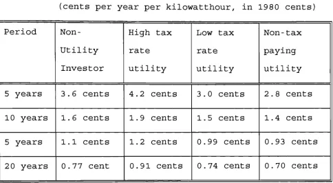
recover its capital in a given period of time. Table 1 compares
reflect different income tax structures [81].
TABLE 1.1
(cents per year per kilowatthour, in 1980 cents)
Period
5 years
10 years
5 years
20 years
Non-Utility
Investor
3.6 cents
1.6 cents
1.1 cents
0.77 cent
High tax
rate
utility
4.2 cents
1.9 cents
1.2 cents
0.91 cents
Low tax
rate
utility
3.0 cents
1.5 cents
0.99 cents
0.74 cents
Non-tax
paying
utility
2.8 cents
1.4 cents
0.93 cents
0.70 cents
One way for an investor to get around high capital recovery
factors is to use long-term bond financing.
Continued federal and state government support of simultaneous
purchase and sale at full avoided costs is viewed by some as the
single most important factor in overcoming industry indecision
to cogeneration [82].
Existing and potential industrial cogeneration participants
include industrial parks, integrated pulp and paper mills, other
process industries (e.g., chemicals, petroleum refining, steel,
food processing, textiles etc.) and heavy oil recovery projects.
rest heavily on a comparison between the cost of cogenerated
electricity (especially, the fuel cost), and the price the
commercial cogenerator pays for its electricity and heat (on
comparative basis). Because of their smaller size, commercial
firms often do not have financial resources equivalent to those
of industrial firms and will be less interested in large scale
projects unless they can be cooperatively owned [83].
Because almost all electric Investors-Owned Utilities Ownership
(IOUs) are in the business of generating electricity, they are
logical potential owners of dispersed generation facilities. The
small size, shorter lead times, and lower capital requirements
of cogeneration systems may provide short-term advantages to
utilities in planning for uncertain demand growth. However, the
PURPA limitations on ownership discourages utility investment in
cogeneration. Moreover, most large utilities do not see dispersed
generating facilities, including cogeneration, as having the
ability to replace future central generating stations, and the
low-earned utility rates of return in recent years may not be
high enough to encourage investment in technologies with
uncertain electricity output.
Full utility ownership may be very advantageous if a utility
faces revenue losses due to industrial or commercial
cogeneration. Moreover, if potential industrial or commercial
cogenerators are unable to burn coal (e.g., due to space or
environmental limitations), or are unwilling to assume the risk
with electricity and steam distribution can centralise the burden
of using alternate fuels. However, the full incremental
Investment Tax Credits (ITC) is not available for utility owned
cogenerators nor are PURPA benefits available if an Investor
Owned Utility (IOU) owns more than 50 percent of the cogeneration
facility.
Alternatively, a utility may decide to participate in joint
venture for a cogeneration facility in order to structure the
ownership in such a way that the investment tax credit and other
tax benefits are diverted to the non-utility participants. In
addition, financing can be structured so that any debt related
to the facility will not appear on the utility's balance sheet.
This structuring would be appropriate for utility-financed
industrial cogeneration or biomass projects [27-29].
Industrial parks also are an excellent application in which
municipalities can foster the development of cogeneration.
Tax-exempt industrial development bonds can be issued without
limit under a specific exemption for the acquisition of land for
industrial parks and its upgrading including water, sewage,
drainage, communication, and power facilities prior to use.
Cogeneration facilities (including steam distribution lines)
presumably would fall into this specific exemption. The
requirements encourage joint ventures between the exempt entity
and business, but the funds must be used by the non-exempt entity
in a trade or business and payments secured by an interest in
prohibit municipalities from entering into corporate
relationships with the private sector, but independent public
authorities usually can be established to get around such
prohibitions [27] .
Rural electric co-operatives are finding it more difficult to
purchase additional electricity from their traditional sources
(IOUs and federal power authorities) and consequently are being
forced to build or participate in new generating capacity. Within
this context, dispersed facilities (including cogeneration) may
be advantageous due to the shorter construction times, greater
planning flexibility, and lower capital costs. In addition,
alternate energy projects are more readily financed at favourable
terms. As with other electric utilities, co-operatives will
prefer projects that provide most of their additional capacity
during peak demand periods and whose electricity output is not
intermittent (e.g., bio-mass, hydroelectric, and industrial
cogeneration projects) [27].
Integration of DSG
For effective operation as part of the utility, a DSG must be
integrated. Integration is defined as follows:
1) a DSG connection to a utility system in which provisions
are made for protection of the DSG as well as the system
2) the operation of the DSG as a managed part of the total
A single DSG unit of relatively small output, or a number of DSG
units of whose aggregate output is small, may be connected to a
system without being integrated [84] i.e, they may be connected
but not integrated as a managed part of the supply mix.
Integrated operations require interaction among the DSGs and the
power system, including the electric utility's bulk supply
systems.
Operational Problems
Cogeneration has impacted the utility generation due to their
base load mode of operation. This base load usually compounds the
utility's daily unit commitment problems associated with unit
cycling, control reserves, and minimum load. The utility
experiences a significant decrease in operating flexibility. Base
load cogeneration affectively removes constant load of this
utility. The worst case scenario is a cogenerator who sells to
the utility only during the off peak, termed off peak dumping.
To avoid this undesirable situation, four different types of
contracts are advised [31-33]:
Firm capacity contracts
Non-firm energy sales only contract
Wheeling contracts
Combination of the above
The operational problems from cogenerator's point of view are
that the basic philosophy behind design of QF generating
utilities. Where the utility must design to meet the growing and
periodically swinging electrical loads, the QF's concerns lie
primarily with meeting thermal demands of manufacturing
processes. Design of electrical capabilities then follows, but
does not usually constitute the primary design constraint.
It is often difficult to comply with the expectations of and
rules imposed by utilities. In some cases, this compliance is
realised at significant economic expenses [2,4].
IEEE formed a Working Group on Current Operational Problems
(COPS) with the goal of focusing attention of the industry on
problems faced by those who are involved in actual power. Eight
system operational areas are identified:
operations planning
normal systems operations
emergency system operations
system restoration
interconnections and pooling
dispatcher selection and training
system operations management
control centre design and maintenance
The group surveyed, conducted numerous technical sessions and
published papers [39-45]. The mathematical modelling aspects of
various types of cogeneration facilities along with the linear
program optimisation procedures implemented to arrive at optimum
The aspects of energy management most impacted by DSG are
associated with real time control. Automatic generation control
(AGO can be influenced by the addition of DSGs within the
control area. The position of a schedulable DSG is dependent upon
considerations of economic dispatch, and will also depend on the
resource of the DSG. AGC is affected in two ways by unschedulable
DSGs. First, the position in the loading order must be
determined, but unlike the case of a schedulable DSG, the
addition of a considerable penetration of uncontrollable power
sources could influence existing generation [5].
If a DSG has independent voltage control capability, it can and
must be operated cooperatively with any method of DSG voltage
control on existing power system. Protection of radial feeders
is generally by breakers or reclosures at the distribution
substation, tripped by the action of an overcurrent relay.
Protection of laterals and transformers is generally by use of
fuses, including current limiting types [5, 15-17, 57] . Intertie
protection schemes using undervoltage, overvoltage,
underfrequency, overfrequency, voltage-controlled or voltage
compensated, battery/DC undervoltage, reverse power are reported
by the Power System Relaying Committee of IEEE. The committee has
prepared a consumer-utility guide to establish a common
understanding amongst those involved in the intertie design [51,
52-56, 61].
Some changes in the safety practices and protection hardware are
switches and lock-out disconnect switches at the DSG
installations would reduce the size of feeder sections with DSG
and prevent the re-energisation of a de-energised feeder section
during maintenance. Because of DSG infeed to faults, fuse sizes
may need to be increased and reclosure settings delayed to
prevent damage to DSG devices operating out of-phase with the
utility system following the occurrence of a system disturbance.
The placement of capacitors to correct the power factor must take
into consideration the possibility of DSG islanding and resonant
overvoltage situations [28].
Automated systems and microprocessor-based protection packages
may be a more practical and safer method for controlling the
operation of DSG devices and protecting the distribution system.
DSG in significant concentrations can have beneficial effects at
the distribution feeder level in terms of reduced voltage drop,
losses, and breaker currents [28].
Before 1970 utilities used traditional planning that stabilised
along a number of lines [29, 36]:
* Cost of fuel was constant or declining in real and often in
current dollars;
* Economics of scale dictated even larger power plants;
* Financing needs were well understood, relatively stable, and
* Heat rate improved regularly as power plant design was
improved;
* The price of electricity declined;
* Load grew at 7% each year;
* Regulatory/industry interactions and dynamics evolved
accordingly.
* Utilities were financially sound, and concern was for minimal
consumer cost.
As uncertainty is the very essence of the problems facing utility
management today, a new approach for planning evolved, known as
the SMARTE (Simulation, Modelling and Regression, and Tradeoff
Evaluation) strategic planning methodology. SMARTE was developed
specifically to address decisions involving conflicting
objectives, uncertainties, as such disparate issues as fuel,
economics, environmental implications, reliability, etc
[47-50,30,35].
Transient studies due to switching, fault conditions and
islanding on a distribution feeder connected to DSG are
negligible so far [11-15, 3] .
1.2 Aims of the thesis
The thesis describes in detail the modelling of a three phase
multi-section distribution feeder, using PI configuration and
mutual couplings between phases, from the line constants. It also
phase induction generator, several inductive loads, a capacitor
bank and circuit breakers connected to the distribution feeder.
The fourth version of the IBM-PC Electro-Magnetic Transients
Program, known as Alternative Transient Program (ATP4) was used
to study the fault and switching transient analysis of the
distribution feeder. The main objectives are:
(1) To develop mathematical and digital techniques to
simulate distribution feeder of industry like SECV
connected to a DSG like induction generator.
(2) To display graphically the transient voltages and
currents at interesting points on the feeders under
several types of fault and switching conditions.
(3) To create situation for islanding of the induction
generator and display graphically the current
supplied by the generator to the loads.
(4) To study the effect of two induction generators,
connected to the feeder at two points, on fault
transients and the essential need to modify the
capacitor bank.
(5) To investigate the changes needed in the protection
components as a result of the connection of the DSG
(6) To report the operation and planning aspects of the
power supplied to feeder connected to DSG.
The mathematical theory on which the models are based and the
explanation of the Alternative Transient Program are described
in Chapter 3.
The data used and the mathematical computations are shown in
Chapter 4.
Chapter 5 contains the graphical plots of transient voltages and
currents during switching and fault conditions. It also offers
an explanation to the shape of the plots and draws valuable
conclusions.
Chapter 6 deals with the operational, control and planning
aspects of the distribution feeder connected to the DSG. It
includes voltage control, reliability, harmonics, earthing, and
contractual matters between the private generator and the
utility. Technical aspects of interconnections are also
considered.
Chapter 7 derives the conclusion of the research and also offers
2.0 Introduction
Transient phenomena plays an important role in power system
networks. This chapter describes a method which was developed
for solving transient phenomena in multi-phase system on a
digital computer [34]. The method is based on step-by-step
integration procedure for lumped parameters and on Bergeron's
idea [98] for lossless lines. Switches with changing positions
are included in the study. The line parameters, which are part
of the input data are for the transient study, are obtained by
calculation. The formatting for computations in ATP4 is given
in Appendix A.
2.1 The solution of transient phenomena
The problem of transient phenomena is to find the voltages u(t)
or current i(t) as a function of time t for a given network.
It is obvious that a discretisation of the problem is necessary
when using digital computers. Instead of a continuous history
in time t, only a sequence of snapshot pictures at discrete
intervals At is obtained. The discretisation interval At is
approximated by simple differences
2.2 Single-phase network
The method, which will first be described for single-phase
networks, can solve any linear network consisting of branches:
1. resistance R
2. inductance L
3. capacitance C
4. lossless lines (distributed constants L', C, per
unit length).
>
* _ - i
Fig. 2-1. Single-phase network
The configuration of Fig. 2-1 will be used for illustration.
It contains all four types of branches and may be a part of a
larger network. Suppose that the instantaneous voltages and
currents have already been calculated at time intervals At up
step-width At will be assumed constant. At any time t the sum of the
currents leaving node 1 through the connected branches must be
equal to the injected current i1#
1 1-2 <t> + i » ) J (t) ^ (t) _ J (t) M )
+ 1^3 + i1 - 4 + 1^5 - i1 u ;
Nodal equations will be used. For node 1 it is found by
expressing the individual branch currents in equation (1) as
a function of node voltages.
2.3 Branch equations
(a) Lossless line.
For the lossless lines equation (2) exists
du=L/di
' dx dt (2)
di _r/du ' dx~ dt
with x = distance on the line from some arbitrary chosen
point
u = u(x,t) = instantaneous voltage at distance x and
time t
L' = inductance per unit length
C = capacitance per unit length.
dPu _L/C,d 2
u
dx2 dt2
(3)
dx2 dt2
The general solution, first given by D'Alembert, is:
i = F(x - vt) + f(x + vt) (4a)
u = ZF(x - vt) - Zf(x + vt) (4b)
with F(x - vt) and f(x + vt) being arbitrary functions of the
variable x - vt and x + vt. F(x - vt) can be interpreted as a
wave travelling at velocity v in the forward direction and
f (x + vt) as a wave travelling in the opposite direction. In
equation (4) new parameters have been introduced, namely
surge impedance = / (L'/C) (5a)
and velocity of wave propagation
v - 1/ V(L'C') (5b)
Equations (4a) and (4b) can be algebraically changed in the
following forms:
u + Zi = 2ZF(x - vt) (6)
u - Zi = -2Zf(x + vt) (7)
u + Zi is constant when x - vt is constant and u - Zi is
constant when x + vt is constant, x - vt and x + vt are called
the characteristics of the differential equations.
Equation (6) may be interpreted in the following way: Let a
with wave velocity v. Then x - vt and consequently u + Zi
along the line will be constant for the observer. Let the
travel time T be defined as the time it takes a wave to travel
from one end of the line to the other,
r = 1/v = 1//(L'C) ( 8 )
where 1 is the length of the line. Then, on line section 2-1
in Fig. 2-1, the expression u + Zi encountered by the observer
when leaving node 2 at time t -r must be the same when arriving
in node 1, that is,
u2 (t
"T) + Z.i^""^ = Ul (t>
+ Z.{-±^) (9)
From equation (9) the branch equation for i,,_2 is obtained,
±^2it} = (1/Z) . u /0 + const1.2(t-T> (10a)
with a constant term, the value of which is known from the
"past history" at time t - T,
const1.2<t"T) = -[(1/Z). u2(t_T) + izV**0 ] <10b)
Equation (10) is an exact solution for the lossless line in
terminal 1. This was the expression used by Bergeron for his
graphical method [85].
l
2 - l
(t)
- >U (t )
"V-B
^A-}^
G=l/Z
L
1-2
_Ct)
U
(t)
A= const2.1
(t
"r) ; B= const1.2 (t
"T)
Fig. 2-2 shows the equivalent circuit for the terminals, which consists of a conductance G = l/z from each node to ground. The nodes are linked only indirectly by means of fictitious
current sources with known values, determined from the past history of the opposite terminal.
(b) Inductance L
For inductance L of branch 1-3 in Fig. 2-1, equation (11) is obtained:
u
i~u3 = L'—jf- (Ha)
from which i ^ at time t is obtained by integration:
ii? =iiVAt,+-|. / (u±-u3)dt (lib)
t-At
Since the voltage drop u, - u3 is only defined at discrete
points, an interpolation between t - At and t is necessary. With linear interpolation equation (lib) becomes
i
i-3(t) - ii-s""*0 +(At/2L){Ul (t
-At> -u3 (t
-At> + U l c t )
- u3 (t
>} (12)
expected to decrease by a factor of 1/8. The trapezoidal rule
for integrating equation (lib) is identical with replacing the
differential quotient in equation (11a) by a central difference
quotient at midpoint between t-At and t with linear
interpolation for u. Equation (12) gives the branch equation
for i,,_3 :
i ^ 0 = (At/2L) [u/0- u3
(t)
] + const,. (13a)
I J C t ?
** *?%*--**
«£-Mr-W-Mr-Mr-M--Mi-M-M'M--3t-Mr-Mr-M--M-»«-M-34-»tM'-M-««-i
t r a p e z o i d r e p l « c I n s i n t e y r a 1 y ( t ) d t
»***+e+e•»*••»«•*€--»«•*«•»«•**••*••€••*-»€• •*•»«•#«•«•••* *«•#*+€
t - •^N, *
"I* r*u n c a -fc I o n fsv-tymr
TL >
Fig. 2-3. Trapezoidal rule for integration
The constant term is again known from the past history:
(t-At)
u (t-At) ] (13b)
const^1"4 0 = i1.3 (t
-At)+(At/2L) [Ul
An equivalent circuit corresponding to equation (13) is shown
in Fig. 2-4. It is a conductance G = At/2L between nodes 1 and
3 with a parallel fictitious current source of known value.
( t - - ^ t )
G = C _ ^ t ) / 2L
<r
(t)
l
3 - l
(c) Capacitance C
For the capacitance C of branch 1-4 in Fig. 2-1, the integral
form is:
r - u r =
U l^ « -
U 4^ «
+ (- | ) . / i^dt d4)
ux (t)
-u4 {t)
= u1
( f c
-A f c )-u4 ( f c
-A f c ) + (At/2C) [i^l+il^] (15)
This indicates linear interpolation for i. The truncation error
is analogous to that of the inductance. From equation (15) the
branch equation for i1-4 is obtained:
i^l = (2C/Afc) [u1 (t,
-l^(th+coI2sfc1
(
£At, (16a)
with the constant term :
const¥;Lt) = -(2C/AC) [ui-At)-u4(fc-At)]-iifc4"At) <16b)
An equivalent circuit corresponding to equation (16) is shown
in Fig. 2-5. Its form is identical with that for the
conductance. A conductance G = 2C/At between nodes 1 and 4 has
a parallel fictitious current source of known value.
(d) Resistance
For the resistance R of branch 1-5 in Fig. 2-1 the current is
given by :
i ^ w = (l/R) [u/r) - u5
ct
(t- - ^ t )
G = 2 C/£± t
4 y . (t
Fig. 2-5. Equivalent circuit for capacitance
2.4 Nodal equations
Inserting equations (10), (13), (16) and (17) into (1) gives the linear equation for node 1:
[1/Z + At/2L + 2C/At +1/R] .u/0 - (At/2L) .u3 (t)
- (2C/At) .u4 (t)
-(1/R) .u5
(t)
= i / " - [const,.^*"0 + const^^'^ + const,./*"*0] (18)
For a general network with n nodes a system of such linear equations can be formed; in matrix notation
Y.U(t) = I(t) - K (19)
where Y
a(t)
j(t)
K
= nodal admittance matrix
= column vector of the n node voltages at time t = column vector of the n injected node currents at
time t
made up of the "past-history terms" const.
The admittance matrix Y remains constant as long as At remains
unchanged. It is real symmetric because the network is purely
resistive with the equivalent circuits of Figs. 2-2, 2-4 and
2-5. Its formation follows the same rules known for the nodal
admittance matrix in steady state analysis. The building
algorithm can be shown more systematically with the use of
incidence matrices, relating branch quantities to node
quantities and vice versa.
In equation (19) part of the voltages will be given and the
others will be unknown. Let the matrices and vectors be
subdivided accordingly into a subset 'a' for nodes with unknown
voltages and subset 'b' for nodes with known voltages. Then
equation (19) becomes
Yaa Yah
^ba. ^bb\ *
'u^'
ui'\
r r < t ) '
-'•a
r(fc)
b
Ka
K
>
from which the unknown vector Ua
(t)
will be found by solving
Ua(t) _ [Ia(t) . Kg . Yab.Ub(t) }/ Yag (21)
This is simply the solution of a system of linear equations for
each time step with a constant coefficient admittance matrix
Y , provided At is not changed. The right sides must be
calculated for each step with the injected currents in Ia(t),
the voltage sources in Ub
(t)
2.5 Practical computation
The problem of solving eqn. (21) is analogous to the steady
state load flow solution with the impedance matrix or the
triangularised admittance matrix. Instead of the iteration
steps in the load flow solution time steps has been used.
Equation (21) is best solved by initially triangularising Yaa
once and for all and extending the triangularisation process
to the right sides in each step with back substitution to get
Ua (t)
[Fig. 2-6] .
(2)
/1\
Initially:
(1) t r i a n g u l a r i r a t i o n Ya a
\|/
">v
a a In each step :1. t r i a n g u l a r i z a t i o n process on right sides
2. hacksuhstitutiun
Fig. 2-6. Solving linear equations with changing right side
Only a few elements in Yaa are non-zero. This sparsity should
be exploited by storing only the non-zero elements of the
triangularised matrix in compressed form. The savings in
computer storage and computing time are impressive and can be
optimised with an ordered elimination scheme.
Should the nodes be connected exclusively via lossless lines,
with lumped parameters R, L, C only from nodes to ground, then
Y becomes a diagonal matrix. As a consequence the equations
technique automatically leads to this simplification, without
having to restrict the generality of the network.
The construction of the column vector for the right sides in
each is mainly an organisational problem. The given node
currents are entered into Ia
(t>
and the given node voltages into
Ub(t). The values may be read in point by point or calculated
with standardised functions (sine curve, rectangular wave
etc.). There are cases where the excitation may come from
voltages only (i = 0) or from currents only (all nodes belong
to subset 'a' then) or where there is no excitation at all
(e.g. discharge of capacitors). Lighting strikes might best be
represented as current sources. The past history is entered
into Ka.
2.6 Extension to multi-phase network
The method can be used to include multi-phase circuits by
formally replacing scalar quantities with matrix quantities.
This generalisation is straight forward for lumped parameters.
For lossless multi-phase lines the coupled phases quantities
will be transformed into decoupled modal quantities. This
linear transformation is similar to that of symmetrical
components in steady state analysis.
2.6.1 Lumped parameters with mutual couplings